Article

A Conceptual Model for Spatial Grain Size Variability on the Surface of and within Beaches

1
Department of Biology, Franklin and Marshall College, Lancaster, PA 17603, USA
2
Field Research Facility, Coastal Hydraulics Laboratory, USACE, Duck, NC 27949, USA
3
Hydraulic Engineering, Delft University of Technology, 2628 CD Delft, The Netherlands
*
Author to whom correspondence should be addressed.
J. Mar. Sci. Eng. 2016, 4(2), 38; https://doi.org/10.3390/jmse4020038
Submission received: 1 February 2016 / Revised: 30 March 2016 / Accepted: 22 April 2016 / Published: 25 May 2016
(This article belongs to the Special Issue Coastal Morphodynamics)

Abstract

:
Grain size on the surface of natural beaches has been observed to vary spatially and temporally with morphology and wave energy. The stratigraphy of the beach at Duck, North Carolina, USA was examined using 36 vibracores (~1–1.5 m long) collected along a cross-shore beach profile. Cores show that beach sediments are finer (~0.3 mm) and more uniform high up on the beach. Lower on the beach, with more swash and wave action, the sand is reworked, segregated by size, and deposited in layers and patches. At the deepest measurement sites in the swash (~−1.4 to −1.6 m NAVD88), which are constantly being reworked by the energetic shore break, there is a thick layer (60–80 cm) of very coarse sediment (~2 mm). Examination of two large trenches showed that continuous layers of coarse and fine sands comprise beach stratigraphy. Thicker coarse layers in the trenches (above mean sea level) are likely owing to storm erosion and storm surge elevating the shore break and swash, which act to sort the sediment. Those layers are buried as water level retreats, accretion occurs and the beach recovers from the storm. Thinner coarse layers likely represent similar processes acting on smaller temporal scales.

1. Introduction

Grain size varies on a natural beach and observations of different sand sizes and their spatial and temporal distributions are well documented (e.g., [1,2,3,4,5,6,7,8,9,10,11]). Recently, Gallagher et al. [10] found that the spatial distribution of sand grain size on the surface of the beach at Truc Vert, France was correlated with morphology. Specifically, coarse sediment was found around rip channels, where flows were strong, and the finest sediment was found high on the intertidal beach where wind was the most common transporting mechanism. These spatial patterns were also observed to change with changing morphology. For example, as a rip channel and shoal system migrated, sediment was constantly reworked and redistributed by the spatially variable surf zone energy field. To examine grain size variations at a higher temporal resolution, an experiment was carried out along two cross-shore profiles in Monterey, CA [11] where the beach was relatively steep (slope 1:7.5) and had a vigorous shore break (where surf zone waves crash dramatically and finally, driving the swash run-up, and where there is often a morphological step). During that experiment, grain size was observed to be largest in that energetic shore break. In addition, the coarse patch moved up and down the beach with the shore break as a function of tidal fluctuations [11], similar to observations by Ivamy and Kench [6]. Attempts to collect stratigraphic information during the Monterey experiment failed [11]. The limited observational studies connecting dynamic morphology change to stratigraphy (e.g., [8,9,12]) indicate that wave and swash interactions with morphology have been observed to induce changes in sediment stratigraphy over a range of temporal and spatial scales, from wave-by-wave and cm-scale changes [8], to tidal and 10 s of cm-scale changes [5,9], to storm and seasonal and m-scale changes [12]. However, most experiments acknowledge that stratigraphy sampling should have been deeper [5,9], or more time or higher frequency measurements would have been useful [8], or they didn’t have direct hydrodynamic measurements [12].
Despite the basic understanding that sediment across a beach is often highly variable in space and time, a mean grain size and spatial uniformity is often assumed in morphology modeling studies to simplify sediment transport calculations (e.g., [13,14,15,16,17,18,19,20,21]). In fact, Soulsby et al. [21] identified grain size as having the largest uncertainty of any sediment transport model input parameter. What remains unclear is the severity of the penalty, with respect to morphology modeling skill and, in nature, how sensitive beach and nearshore morphodynamics are to variations in sediment characteristics both on the surface and in the shallow stratigraphy. Gallagher et al. [22] modeled cross shore bar migration and found that the model had higher skill when cross shore-varying (surface) grain size was used instead of a single mean size for the whole beach profile. Ruessink et al. [23] modeled a coarse foreshore as immobile, because the relatively fine mean size used in the model predicted unrealistic, excessive erosion in that energetic region. Preliminary work by Gallagher et al. [24] showed that by including a coarse-grained, less-mobile patch in the swash, the dynamics of the offshore sand bar were altered. That study suggests that local grain size and its patchiness may impact the dynamics of the whole beach profile. If true, one would expect that variable layers, which are distributed throughout the shallow stratigraphy and the result of earlier time periods with differing wave energy and swash location, will impact overall profile dynamics as well.
Reniers et al. [11] used a multi-grain size module in Xbeach (an open source nearshore morpho- and hydrodynamics model; [18]) to include spatially and temporally varying grain size in beach profile predictions. They modeled the coarse patch that was observed in Monterey and found that the high levels of turbulence and strong (but intermittent) currents in the shore break and swash were effective at winnowing and moving finer sediment both up and down the beach, leaving coarse sediment in place at the base of the swash. Reniers et al. [11] used a uniform distribution (equal amounts of the different sizes) in each layer to commence each model run because information about stratigraphic layers at Monterey was not available. In that study, modeled flows would encounter well-mixed sediment and redistribute it, successfully recreating observed surface sediment spatial variations.
In the present study, stratigraphy in the beach at Duck, NC was measured to document the presence and extent of grain size spatial variation within the bed on a natural beach and to begin to understand how the waves and swash create and then interact with layers of different sediment sizes. Specifically, spatial and temporal variations in the beach elevation and the shallow stratigraphy were examined over a course of a week, before and after a storm event as well as over a tidal cycle, using a suite of sediment cores and beach trenches. These stratigraphic observations were examined in the context of changing beach topography and water levels to understand the role nearshore hydrodynamics may play in creating and/or destroying beach stratigraphy. A conceptual stratigraphic model (including shore break sorting, wave/infragravity-scale bed level fluctuations and shore break translation) is proposed to describe the relationship between swash hydrodynamics at the shore break and the resulting sediment stratigraphy across the beach and foreshore.

2. Materials and Methods

2.1. Experiment

In March–April, 2014, a field experiment was conducted to test an enhanced coring technique, developed to overcome difficulties of collecting sediment cores in the swash, and to sample the stratigraphy across the beach. The experiment was conducted at the U.S. Army Corps of Engineers Coastal and Hydraulic Laboratory’s Field Research Facility (FRF) in Duck, NC. Cores were collected at 8 locations along a cross-shore profile, which spanned from the bottom of the dunes into the deep swash (Figure 1a,c and Figure 2a). The profile was sampled on five occasions: before and after a storm on 25 March and 27 March, after a smaller wave event on 28 March, and at high and low tide on 1 April (Figure 1b). After the coring was finished (2–3 April), two large trenches were dug in the beach to examine and photograph stratigraphy and to put the core observations in context (Figure 1a). From 27 March to 2 April, a simple experiment was conducted to examine the depth of disturbance of the surface sediment (Figure 1a). RTK-GPS (Real Time Kinematic Global Positioning System) elevation surveys of the experiment area were conducted daily both with a backpack and the CRAB (Coastal Research Amphibious Buggy; www.frf.usace.army.mil) (Figure 1a,c). In addition, over 27–28 March, a lidar was mounted on the dune to measure waves, swash run-up, and beach elevation changes along a cross-shore profile line adjacent to the core cross-shore profile. In addition to these experiment-specific measurements, current and wave data were being collected by the FRF in 2 m, 4 m, and 8 m water depths.

2.2. Cores

Previous efforts to collect cores in the swash met with mixed results. Because the sediment in this region at Duck (and in Monterey) is coarse and highly fluidized by the constant motion of the shore break and swash (Figure 2b), so retaining sediment in core tubes after collection proved to be difficult. To address this, aluminum core barrels were fitted with custom-designed, reusable core catchers, which were riveted into the base of each barrel (Figure 2c). Crafted from a single sheet of stainless steel, the catchers are fitted with a cutting edge on the base, an internal rim to brace the barrel, and taper to a series of thin, laser-cut “fingers”. The fingers unfold and press along the internal wall of the barrel by the force of sediment entering the barrel during coring. Then, they subsequently fold closed by the weight of the sediment in the core barrel, effectively forming a solid plug once core extraction begins (Figure 2c). In addition, prior to extraction, the fully penetrated core was filled to overflowing with seawater to create suction and sealed with a standard 3-inch plumbers plug. Once extracted, a plastic cap was taped over both ends to further seal the core. The cores were kept upright until they were processed.
In addition to collecting surveys, the stable, amphibious CRAB was used as the sampling platform for vibracore collection (Figure 2a). A Briggs and Stratton 5 Hp engine with a modified concrete shaker (to vibrate the cores for penetration) was mounted on the CRAB ~3 m off of the ground (Figure 2), allowing the engine to stay dry throughout the coring process, even when collecting cores in the surf. The operation still required personnel to be in the water to guide the core barrel into the sand, therefore core collection was constrained to ~1 m water depth (Figure 2a,c). Using these special adaptations, a total of 36 cores were collected on four different days over about a week. Cores were not collected at exactly the same locations on successive days, but instead were spaced 1–2 m from the previous spot, alongshore and on the same elevation. This was done in part because the coring process disturbs the stratigraphy, and in part because reoccupying the exact same positions is nearly impossible. Accordingly, cross-shore and alongshore trenches were dug to examine small-scale spatial variability in stratigraphy, and are described more in Section 2.4, below.

2.3. Core Processing

Once returned to the FRF, the core barrel was cut just above the sediment line to allow the excess water to flow out. The top of each barrel was stuffed with paper towels to minimize sediment movement, and then the cores were temporarily placed horizontally in order to remove the core catchers for future use. Once removed, the base of each barrel was also stuffed with paper towels to minimize sediment movement and slow water loss, then capped and taped. If not opened immediately, the cores were stored upright in a refrigerator.
For processing, each core was laid horizontally in a steel trough and cut in half with a skill saw by cutting just the metal barrel on each side. Care was taken not to allow the blade to penetrate into the sediment. Cores were split open, photographed and described qualitatively. One half of the core was sampled and bagged for later analysis. Samples were collected every 10 cm as well as at significant changes in lithology. The other half of the core was placed on a conveyor belt and photographed using a digital imaging system for estimating grain size (Figure 2d).

2.4. Digital Imaging System

A fixed frame above the conveyor belt described in Section 2.3, above, was used as the reference/photo point (Figure 2d) for the digital imaging system (DIS). The core was moved using the conveyor belt and images were taken every cm moving down the core. Each image is approximately 2 × 2 cm (or ~2000 × ~2000 pixels), allowing an approximately 50% overlap between successive down-core images.
For analysis, each image is split into horizontal (cross-core) sub-images or plaquettes that are 200 × 2000 pixels or 0.2 × 2 cm. The plaquettes are used to estimate mean grain size for that small flat layer. There is 75% overlap between each plaquette, giving 34 overlapping plaquettes and resulting in a running average of grain size moving down the image. Ultimately, each image provides a profile from top to bottom, with 34 values of mean grain size. Because the different images overlap by approximately 50%, multiple estimates of grain size are provided in different depth bins. In addition, images were taken side-by-side along the open core face, further increasing the number of estimates in each depth bin. DIS data have been found to be noisy, but averaging, overlap, and multiple photos have been shown to significantly improve DIS mean grain size estimates [10]. For this study, final smoothing was done by averaging all estimates in 0.5 cm depth ranges. Grain size was estimated from images using the autocorrelation technique developed by [25], together with recently developed grain size image calibration curves for Duck, NC.

2.5. Trenches

To put the core observations in context, two large trenches were dug in the dry beach using a backhoe. One trench was dug perpendicular the shoreline (trench 1) and the other was dug parallel to the shoreline (trench 2). The total length of trench 1 was about 15 m and it cut across the side of the horn of a beach cusp (see Figure 1a for approximate locations). At its seaward end, trench 1 was about 1 m deep. At its landward end, it was ~1.5 m deep. The seaward-most extent of the trench was limited by the water table, which caused slumping within ~10 m of the swash. The landward extent of the trench was constrained by the dune. The alongshore trench was dug just above the high tide line on the berm and was dug across the cusp trough and to the crest of the next beach cusp. Trench 2 was ~30 m long, ~2 m deep, and reached down to the water table. Once dug, the stratigraphy was photographed every ~1 m along each trench, and general features were described and drawn.

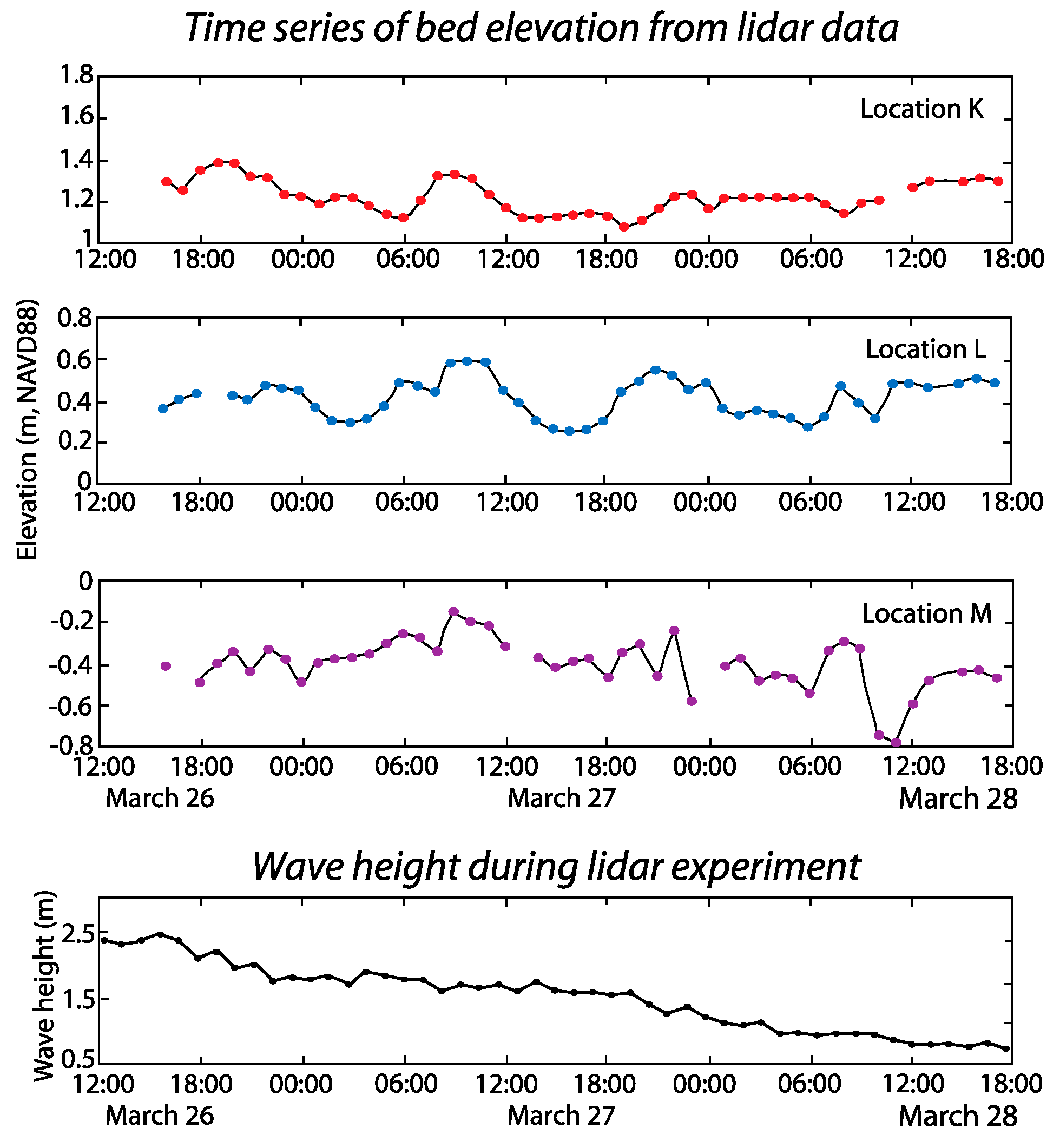
2.6. Changes in Beach Elevation Change and the Active Layer

A simple test was conducted to examine thickness of the active layer of sediment in the swash together with changes in beach surface elevation. Metal washers were placed over metal rebar rods, which had been driven into the sand on a cross-shore profile approximately 20 m north of the coring profile (Figure 1a). The distance from the top of the rod to the sand level, and from the sand level to the depth of the washer, was measured on a daily basis. Because the stainless steel washer is denser than the sediment, it will settle to the bottom of the moving layer as each swash crosses the beach, lifting, moving, and re-depositing the active sediment. This simple test gives a measurement of the deepest depth of sediment motion (i.e., the active layer or depth of disturbance) of the bed over the time period of measurement (here: 1 day). This method is similar to previous efforts to quantify active layer thickness (e.g., [6]).
To examine changes in surface elevation at finer scales than that permitted by the washer technique (and without the potential for scour) a Riegel terrestrial lidar scanner (LMS-z390i, 1550 nm laser with a 0.3 mrad beamwidth) was used to measure surface elevation of the beach at 2 Hz for 30 min starting at the top of each hour. Specific details regarding lidar operation and limitations of the specific system are detailed in [26]. To estimate beach elevation, data were transformed from the scanner coordinate system (angle and range) to rectified Cartesian coordinates (local coordinates for the horizontal and NAVD88 coordinates for the vertical) using a transformation matrix determined from scans of GPS-surveyed reflectors. It should be noted that because the lidar measurements were made ~35 m south of the depth of disturbance experiment, detailed comparisons between the methods are not appropriate. Accordingly, only general trends will be compared.

3. Results

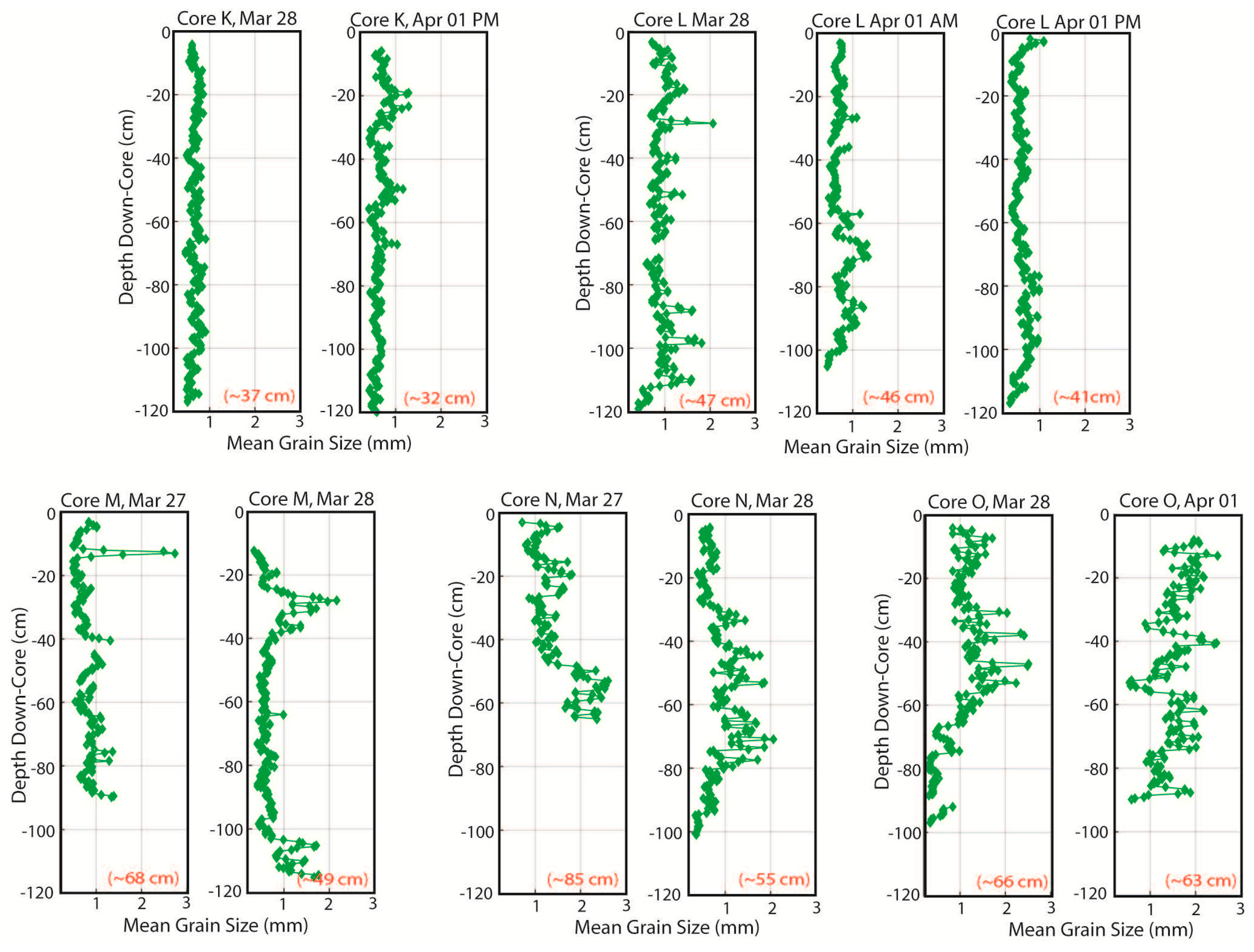
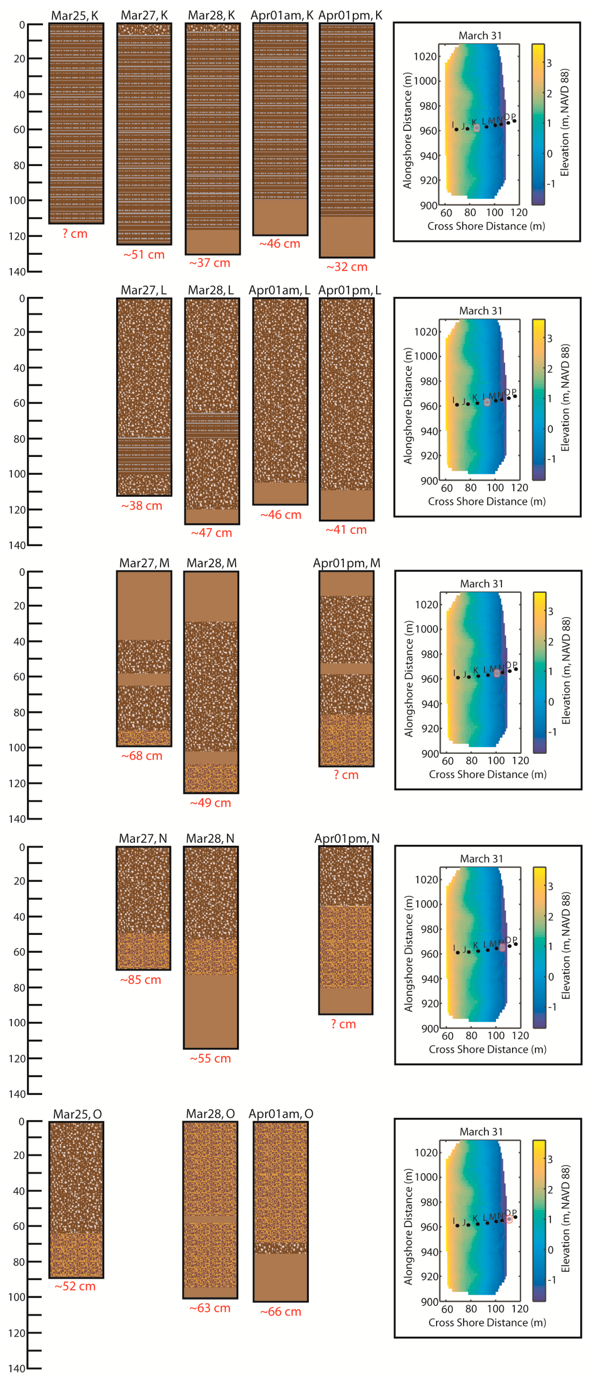
3.1. Core Observation

Figure 3 shows the results from the DIS grain size estimation, giving profiles of mean grain size with depth in the cores at the different times and locations. The wide range of grain sizes observed varies not only spatially and temporally between core sites but also within individual cores. This illustrates the inadequacy of using a single grain size to characterize the beach.
The length of the cores, and the thickness and position of observed layers, may be somewhat altered due to compaction created during the coring process. As the core tube is vibrated and driven into the ground, the sediment in the tube is compressed. In addition, when the core is removed from the ground, water can flow out of the barrel, potentially disturbing the sediment layers within the barrel. The numbers shown in red in Figure 3 represent the difference between the ground surface along the edge of the core barrel (the actual depth of penetration; marked on the barrel prior to the barrel being extracted from the ground) and the top of the sediment inside of the core barrel. Compaction is common during coring and the amount of compaction in each core measured during this experiment is consistent with compaction measured previously during other sandy beach coring efforts using similar methodology (e.g., [27,28,29]). Because compaction happens nonlinearly in the core, stretching the core data generally is not done.
Unfortunately, during the coring process, vibration of loose sediment may jostle, rework, and ultimately damage some of the finer layers (≤1 cm). Evidence for the destruction of finer layers comes from the comparison of the cores (both visual inspection and DIS measurements) and observations from the trenches, where cm-scale stratigraphic layers were visually observed. Accordingly, visual and DIS data were used together to help define four distinct sedimentary units, as preserved in the cores: (1) Homogenous Sand (HS), a fine-grained sand (<0.5 mm grain size) often with minor coarse sediment, either as individual grains or as thin (<5 mm) laminae, as well as occasional heavy mineral laminations; (2) Poorly Sorted coarse Sand (PSS), a medium- to very coarse (~0.5–1.3 mm grain size) sand with abundant granules and pebbles but no discernible layering, and that often coarsens with depth down-core; (3) Laminated Sand (LS), a unit comprised of discrete layers (on the order of 1 cm) of both HS and PSS; and (4) Coarse Gravel (CG), moderately well to well-sorted, well-rounded coarse gravel (1–2 mm grain size), with minor med-coarse sand and varying amounts of fragmented shell (see Figure 4 for examples of the sedimentary units). Although discrete laminae of PSS and HS of 1–2 cm or finer were observed in the sediment cores, for the purposes of the core descriptions (Figure 5), only layers of PSS or HS that were at least 5 cm in thickness were considered a discrete stratigraphic unit. Finer layering is defined as LS.
A selection of cores is shown in Figure 3 and Figure 5 that illustrates the major observations from the cores. Higher on the beach, grain size is dominated by finer grains, generally <0.5 mm, and is more uniform with depth. Location K is shown as representative of these more uniform observations at locations I, J and K (Figure 3 and Figure 5). At all three locations, LS is the dominant unit. At K, a thin layer (<10 cm) of PSS is seen on the surface after the large wave event (26 March, Figure 1b) deposited a small amount of coarser material high on the beach. The HS near the bottom of some of the cores at location K is consistent with the observation of finer and relatively uniform sediment high on the beach because HS is a component of LS and was likely deposited during an extended quiescent period. It also is possible that HS is below LS at many or all locations and times, but was not reached with some of the cores.
With increasing distance seaward from the dune, the sediment becomes coarser and more varied, both spatially and temporally. The coarsest material (~2 mm) dominates at the deepest coring location shown (location O) and this layer of coarse material is relatively thick, at least 60–80 cm. Farther offshore, the sediment is once again fine-grained ([30], [11] and from our personal observations, but not sampled). At location N, landward of O but still frequently in the swash zone and shore break (Figure 1c), the coarse layer is also visible, but lies below a PSS layer. This is likely owing to location N being in a highly variable location, sometimes in the lower swash and sometimes directly in the intense shore break.
These data also suggest that over the course of the experiment, the top 20–40 cm of the beach surface was highly variable in time (see the discussion of the active layer in Section 3.3). This is well illustrated by the cores at locations M, N, and O where the top layer of the cores is quite different from day to day (Figure 3). For example, at location N, on 27 March, the grain size in upper 30 cm of the core ranged from 1–2 mm, whereas on 28 March, the upper 30 cm was finer, ~0.7 mm (Figure 3).
The more variable, intermediate elevations on the cross-shore profile are well illustrated by the cores at locations L and M (Figure 3 and Figure 5). Location L is dominated by poorly sorted, downward coarsening sediment. A minor LS unit is observed mid-core on 27 March and 28 March, but not on 1 April, and this could be due to horizontal spatial variability of the layer. The L core collected on 27 March does not show the HS unit at the base (Figure 5, found on 28 March and 1 April), but the layer may have existed below the base of the collected core. The cores at location M have fine material (HS) on the surface, poorly sorted sediment (PSS) over most of their depth, and coarse gravel (CG) near the bottom. These PSS layers, together with the vertical variability at M, represent the reworked and highly changeable sediment observed at this location, which can be in the upper, mid or lower swash or in the shore break, depending on tides, waves and storms.

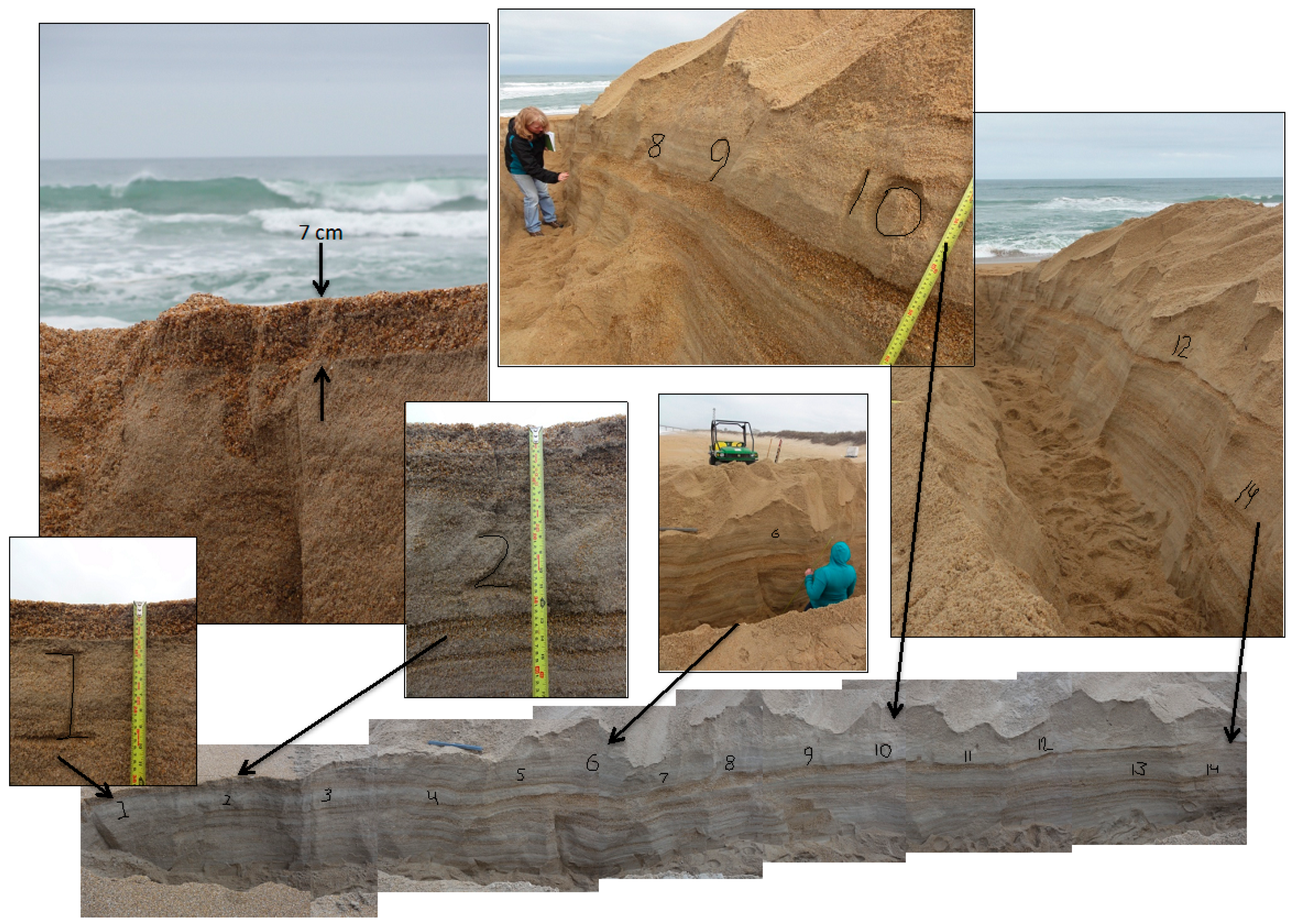
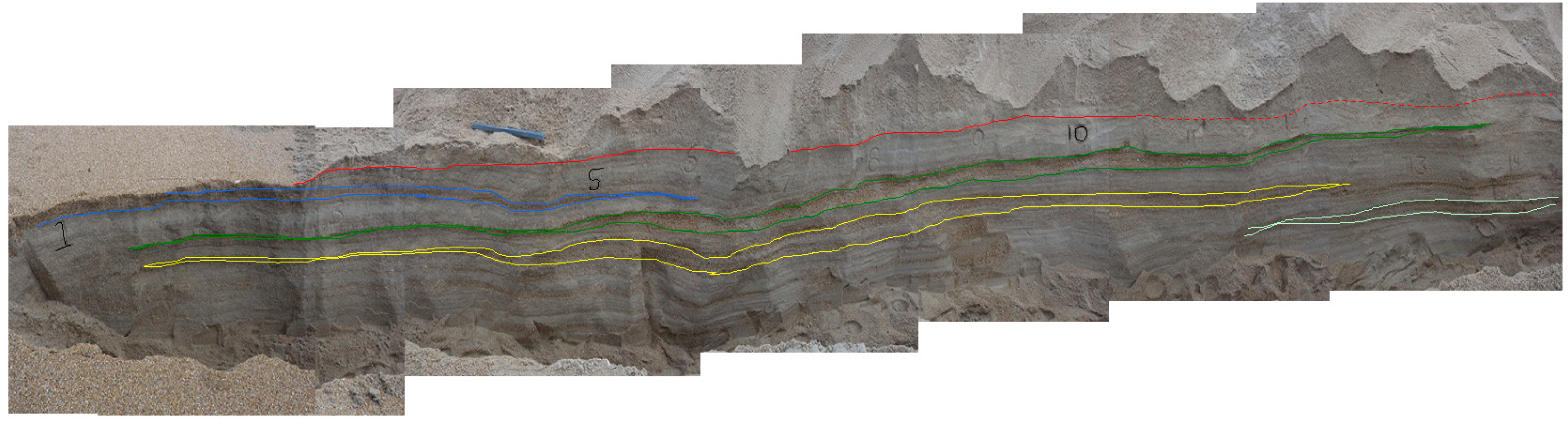
3.2. Trench Observations

Layering of many scales was observed in the trenches (Figure 6). Thick (~2–10 cm) gravel/sand layers were visible (CG or PSS) and are generally attributed to elevated sea level and swash action, likely owing to storm events (e.g., the thick, continuous coarse layer below the “7”, “8”, “9” and “10” in the bottom panel in Figure 6). Thinner laminae (1–2 cm) were also visible but were less distinct and not as well sorted. For example, immediately below the “10” in the top, center photo of Figure 6, but above the thick coarse layer of PSS, are four thin (≤1 cm) layers of finer PSS and HS sediments. The larger, coarser sediment layers are outlined in Figure 7 to emphasize their extent and shape. Overall, these layers form “lenses” of coarse sediment with a cross-shore extent of almost the length of the trench (~10–15 m), and a thickness of roughly 10 cm (Figure 6). These lenses are thought to be owing to shore break and swash acting higher on the beach, and are described in more detail in Section 4.

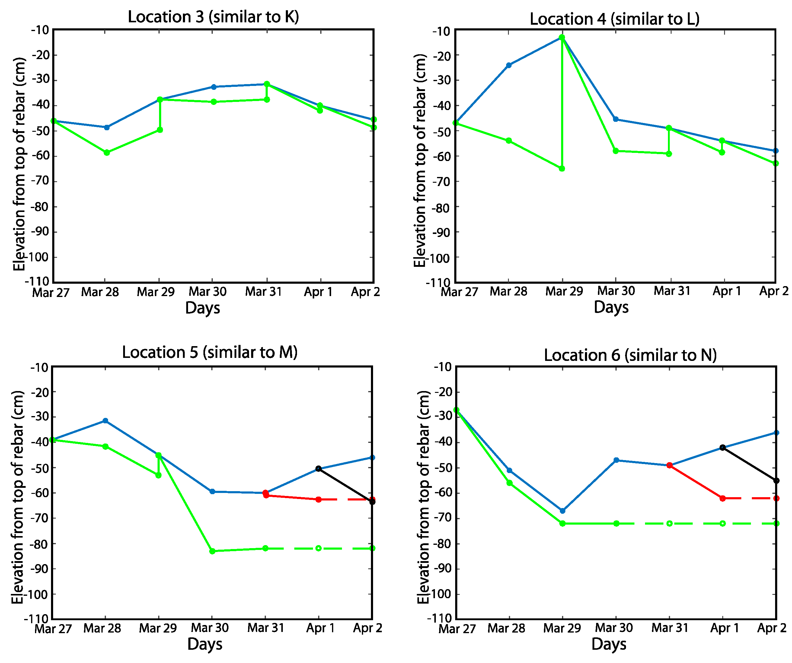
3.3. Depth of Disturbance Observations
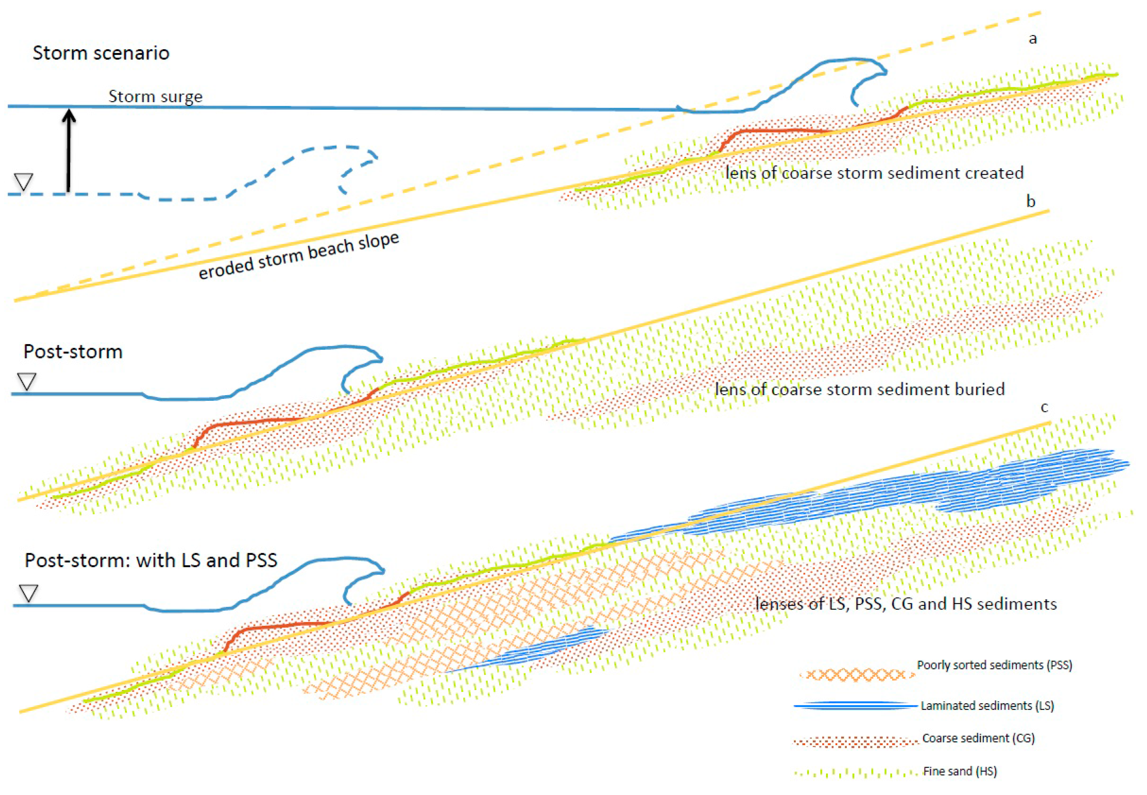
In the shore break and swash, each wave suspends, moves and deposits sediment, thus the processes acting to sort and redistribute different grain sizes are constantly at work. Observations in the literature (e.g., [6,8,9,31,32,33]) indicate that the beach face in the swash is alternatingly eroding and accreting over relatively short time scales. Figure 8 shows about two days of data from the dune-mounted lidar (26–28 March). The time series shows the elevation every hour (the minimum elevation is taken each hour to represent the time window) at three different core locations. The beach elevation is seen to fluctuate by 20–40 cm over the course of a few hours. Indeed, variations in elevation in the swash of up to 15 cm over the course of about 5 min are visible in the lidar data ([31,32] and in the present data set, not shown).
Figure 9 shows the results of the daily depth of disturbance measurement from the rebar array, and this simple experiment also provides insight into the movement of the bed. The blue line shows the daily elevation of the beach surface, which is under-sampled when compared with Figure 8, but still indicates that variations in surface elevation in the lower, active swash are at least 40 cm, even when the waves are small (e.g., 27–29 March, locations 4 and 6; Figure 1 and Figure 9). In the region of the upper swash, those variations are smaller, but still reach ~20 cm at location K (Figure 8 and Figure 9). These data (as well as the traditional cross shore profile surveys in Figure 1c) indicate that the top layer of the beach is highly active and being eroded and re-deposited over relatively short time periods. In addition, the timing and amplitude of the observed elevation change does not seem to be directly related to offshore wave height (Figure 9).
The green, red, and black lines in Figure 9 represent the maximum depth to which the washers moved. Vertical lines indicate when the washer was removed and placed back on the beach surface, while dashed lines indicate that the washer was not found at the next sampling. Lost washers were buried too deeply to retrieve via digging along the rebar, though it should be noted that, in the swash, digging deeper than about 30 cm is difficult because water and sand refill the hole as fast as one can dig. These results indicate that at least the top 10–30 cm of the sand bed in the swash is active, being suspended and re-deposited regularly: on at least a daily, and likely hourly, basis.

4. Discussion

The shore break, where waves break at the base of the foreshore before running up the beach and where there is often a morphological step (Figure 2b), creates intense, turbulent velocities that can suspend finer sediment, allowing it to be transported landward and/or seaward, while the coarser fraction, which is less mobile, remains in place [5,6,7,9,11,20]. This process of sorting with each wave in the shore break is the fundamental process in the conceptual stratigraphic model that is presented here. It can be thought of as the sorting engine and it is illustrated in Figure 10a. The depth of disturbance experiment and the lidar reveal topographic variations of at least 10–40 cm owing to waves reworking the surface in the swash. This erosion/accretion happens over a range of timescales from minutes to hours and reflects the forcing of individual waves varying with the wave-groups and infragravity motions and the response of the beach, slope, and grain size [8,31,32,33,34,35,36]. One effect of this vertical change in beach elevation is to thicken the sorted layer and this illustrated in Figure 10b. Astronomical tides and storm surge translate the shore break across the beach profile (Figure 10c), horizontally extending the region where the shore break sorting engine is working [5,11]. Sediment in this region is systematically sorted by these processes, with finer material being moved away, leaving a lens of coarse sediment (Figure 10a–c). This coarse-grained, well-sorted sediment layer, usually represented by the CG unit (Figure 4 and Figure 5), is thickest where the shore break resides for the longest period of time. Where it was observed at locations N and O (Figure 3 and Figure 5), it can reach thicknesses in excess of 50 cm.
The PSS unit can be thought of as being a poorly sorted precursor to the CG unit. When the sorting engine has not had time to fully sort the sediment or at the distal ends of the shore break sorting region, PSS will result.
Away from the shore break, at the upper edge of the swash, where the water decelerates (or accelerates) as it runs up (or down) the foreshore, sediment also is sorted [8]. As the flows decelerate (on their way up the beach), sediment falls from suspension, coarser sands first, then medium sands and the finest grains are deposited farthest from the shore break, falling out of suspension last. High on the beach, these finer-grained, depositional layers are exemplified by the LS unit (Figure 4). The layers are thin and may be deposited (or eroded) with each wave [8]. Core observations reveal that these layers may vary in the vertical from coarse sand to fine sand because of differences in transport potential from wave to wave, over infragravity periods and position in the swash. Indeed, these two processes ((1) vertical stirring, winnowing and sorting in the shore break and (2) horizontal sorting higher in the swash) are the same mechanically, but the first happens over many waves, reworking and transporting the grains as exemplified in Figure 10. The second happens with every wave, and the separation is immediate and slightly less distinct.
During a storm, large waves often remove sand from the beach, cutting the surface down to a lower elevation, which results in an onshore translation of the water line (and a redistribution of sediment). Additionally, elevated water levels owing to storm surge and wave set-up, translate the mechanisms outlined in Figure 10 farther onshore (Figure 11a). This is the primary mechanism for creating the coarse lenses (Figure 7) observed farther onshore than the swash position would occur under the normal tidal translation (Figure 10c). As water level fluctuates during a storm event, from either falling tides or waning surge, the coarse layer may extend across the beach (either CG or PSS, depending on the time frame). In addition, the mechanisms creating thin, graded layers (LS) may be at work at the highest extent of the swash, also higher on the beach than usual, and finer sediment may be moved seaward and deposited on top of coarser sediment, where the swash usually resides (see, for example, location M on 28 March at 100 cm depth, Figure 3 and Figure 5).
While deposition is important for any observation of stratigraphy, it is commonly assumed that erosion during storm conditions frequently results in the destruction of storm layers in the foreshore and lower beach. Recently, however, researchers have observed beach recovery (accretion) beginning during the height of the storm, as wave heights begin to wane [34,35,36]. These observations suggest that accretion may be occurring even while storm waves and surge are working high on the beach, thus allowing the accumulation and preservation of the coarser storm layer as described in Figure 11a,b.
During more quiescent conditions, data indicate that the top ~10–40 cm or so of the beach at Duck is reworked regularly. A number of recent observations conducted on similar sandy beaches indicate that those beaches eroded and accreted significantly over the course of a few waves to an hour, with elevations fluctuating up and down in the swash (Figure 8 and Figure 9, and studies by [31,32,33]). If there is no net change in beach elevation, these small waves will repeatedly accrete and erode sediment within the active layer. During times of net accretion, such as a summer beach accreting under the influence of small waves, preservation of these thin layers will occur, resulting in LS stratigraphy.
The different stratigraphic units (Figure 4) were defined in order to characterize not only the observed grain sizes but also the temporal and spatial variability of the responsible depositional processes. We suggest that these processes reflect a continuum of forcing processes, which can be represented by these characteristic sedimentary layers. In Figure 11c, the conceptual model is qualitatively redrawn using the four units and possible cross-shore and vertical positions as a function of sorting hydrodynamics. PSS is a poorly sorted unit (Figure 4) and likely reflects sorting and depositional processes that occur between conditions responsible for the quiescent LS and the energetic CG formation. CG is well-mixed owing to strong turbulence in the shore break. LS tends to form at the upper reaches of the swash where more gentle velocities allow grain size sorting on an intra-wave basis. HS layers result from suspension and transport away of well-sorted, finer grain sizes from the most turbulent regions of the shore break, and Aeolian processes likely also play a role in sediment sorting and accretion. Thus, accretion during a post-storm recovery might result in the accumulation of a coarser LS layer or a PSS layer in the mid-swash, CG layers in the lower swash and shore break, LS or even HS layers high on the beach or offshore on top of a preexisting CG layer. These combinations are seen in the preserved lenses and strata in the cores and the cross-shore trench (Figure 3, Figure 5 and Figure 7).

5. Conclusions

It is important to know the range of grain sizes on a beach for sediment transport and morphological modeling, in part so that each fraction can be moved around accurately (e.g., [11,20]). As the redistribution of different grain sizes takes place, the local morphology changes owing to subtle changes in erodibility and transportability. In addition to this direct relationship, as local morphology, grain size and slope change, the hydrodynamics change in response. Thus, grain size, hydrodynamics (turbulence, roughness, infiltration, etc.) and morphology are all interdependent through feedbacks. Further, it is hypothesized that variations in size and sorting of sediment along the foreshore affect larger-scale profile morphology through feedback with forcing wave conditions [24]. The present conceptual model attempts to elucidate the three processes that work simultaneously (Figure 10) to sort and redistribute sediment on the foreshore and beach and explain typical beach stratigraphy. These processes create sedimentary layers, which are observed in the beach and, when exposed, become part of the hydro-, morpho-, and sediment dynamic feedback working on the beach. Further work will explore the relationships between stratigraphy and the feedbacks between related hydrodynamics and morphodynamics.

Acknowledgments

The authors would like to acknowledge support from the National Science Foundation, Geomorphology and Land Use Dynamics (EAR 0952225, EAR 0952163), the Office of Naval Research (N00014-13-1-0621), and the U.S. Army Corps of Engineers (Coastal Field Data Collection program; Morphology work unit). The authors would also like to thank the staff of the Field Research Facility, especially J. Pipes, B. Scarborough, and M. Preisser, for their dedicated efforts and expertise. Thanks to C. Hagen for field support and photography. Special thanks to K. Brodie and N. Spore, USACE-CHL, for collection and processing of lidar data.

Author Contributions

E.G. and A.R. conceived the research. E.G., A.R., H.W. and J.M. designed and performed the experiments. All authors worked on data analysis (E.G. on DIS data, H.W. and M.K. on core analyses, J.M. on lidar data, A.R. on bathymetric and wave data). E.G. wrote the first draft of the manuscript and all authors contributed to the final text and figures.

Conflicts of Interest

The authors declare no conflict of interest.

References

  1. Komar, P.D. Beach Processes and Sedimentation; Prentice-Hall: Upper Saddle River, NJ, USA, 1998. [Google Scholar]
  2. Nielsen, P. Coastal and Estuarine Processes; World Scientific Press: Singapore, 2009. [Google Scholar]
  3. Holland, K.T.; Elmore, P.A. A review of heterogeneous sediments in coastal environments. Earth-Sci. Rev. 2008, 89, 116–134. [Google Scholar] [CrossRef]
  4. Buscombe, D.; Masselink, G. Concepts in gravel beach dynamics. Earth-Sci. Rev. 2006, 79, 33–52. [Google Scholar] [CrossRef]
  5. Hay, A.E.; Zedel, L.; Stark, N. Sediment dynamics on a steep, megatidal, mixed sand-gravel-cobble beach. Earth Surf. Dyn. 2014, 2, 443–453. [Google Scholar] [CrossRef]
  6. Ivamy, M.C.; Kench, P.S. Hydrodynamics and morphological adjustment of a mixed sand and gravel beach, Torere, Bay of Plenty, New Zealand. Mar. Geol. 2006, 228, 137–152. [Google Scholar] [CrossRef]
  7. Mason, T.; Coates, T. Sediment transport processes on mixed beaches: A review for shoreline management. J. Coast. Res. 2001, 17, 645–657. [Google Scholar]
  8. Otvos, E.G. Sedimentation-erosion cycles of single tidal periods on Long Island Sound beaches. J. Sed. Pet. 1965, 35, 604–609. [Google Scholar]
  9. Duncan, J.R. The effects of water table and tide cycle on swash-backwash sediment distribution and beach profile development. Mar. Geol. 1964, 2, 186–197. [Google Scholar] [CrossRef]
  10. Gallagher, E.L.; MacMahan, J.H.; Reniers, A.J.H.M.; Brown, J.; Thornton, E.B. Grain size variability on a rip-channeled beach. Mar. Geol. 2011, 287, 43–53. [Google Scholar] [CrossRef]
  11. Reniers, A.J.H.M.; Gallagher, E.L.; MacMahan, J.H.; Brown, J.A.; van Rooijen, A.A.; van Thiel de Vries, J.S.M.; van Prooijen, B.C. Observations and modeling of steep-beach grain-size variability. J. Geophys. Res. Oceans 2013, 118, 577–591. [Google Scholar] [CrossRef]
  12. Neal, A.; Pontee, N.I.; Pye, K.; Richards, J. Internal structure of mixed-sand-and-gravel beach deposits revealed using ground-penetrating radar. Sedimentology 2002, 49, 789–804. [Google Scholar]
  13. Plant, N.; Holland, K.T.; Puleo, J.; Gallagher, E.L. Predictions skill of nearshore profile evolution models. J. Geophys. Res. 2004, 109, C01006. [Google Scholar] [CrossRef]
  14. Castelle, B.; Ruessink, B.G.; Bonneton, P.; Marieu, V.; Bruneau, N.; Price, T. Coupling mechanisms in double sandbar systems, Part 1: Patterns and physical explanation. Earth Surf. Process. Landf. 2010, 35, 476–486. [Google Scholar] [CrossRef]
  15. Roelvink, J.A.; Reniers, A.J.H.M. Guide to Modeling Coastal Morphology; World Scientific Press: Singapore, 2011. [Google Scholar]
  16. Johnson, B.D.; Kobayashi, N.; Gravens, M.B. Cross-shore numerical model CSHORE for waves, currents, sediment transport and beach profile evolution. In Proceedings of the Great Lakes Coastal Flood Study, 2012 Federal Inter-Agency Intiative, Washington, DC, USA, September 2012.
  17. Nielsen, P.; Callaghan, D.P. Shear stress and sediment transport calculations for sheet flow under waves. Coast. Eng. 2003, 47, 347–354. [Google Scholar] [CrossRef]
  18. Roelvink, J.A.; Reniers, A.J.H.M.; van Dongeren, A.R.; van Thiel de Vries, J.S.M.; McCall, R.T.; Lescinski, J. Modeling storm impacts on beaches, dunes and barrier islands. Coast. Eng. 2009, 56, 1133–1152. [Google Scholar] [CrossRef]
  19. Hoefel, F.; Elgar, S. Wave induced sediment transport and sand bar migration. Science 2003, 299, 1885. [Google Scholar] [CrossRef] [PubMed]
  20. Blondeaux, P. Sediment mixtures, coastal bedforms and grain sorting phenomena: An overview of theoretical analyses. Adv. Water. Res. 2012, 48, 113–124. [Google Scholar] [CrossRef]
  21. Soulsby, R. Dynamics of Marine Sands; Thomas Telford Limited: London, UK, 1997. [Google Scholar]
  22. Gallagher, E.L.; Elgar, S.; Guza, R.T. Observations of sand bar evolution on a natural beach. J. Geophys. Res. 1998, 103, 3203–3215. [Google Scholar] [CrossRef]
  23. Ruessink, B.; Kuriyama, Y.; Reniers, A.J.H.M.; Roelvink, J.A.; Walstra, D. Modeling cross-shore sandbar behavior on the timescale of weeks. J. Geophys. Res. 2007, 112, F03010. [Google Scholar] [CrossRef]
  24. Gallagher, E.L.; Reniers, A.J.H.M.; Wadman, H.; McNinch, J.; MacMahan, J. Onservations and modeling of grain size variability on and in a steep beach. In Proceedings of the AGU Ocean Sciences Meeting 2014, American Geophysical Union, Honolulu, HI, USA, February 2014.
  25. Rubin, D.M. A simple autocorrelation algorithm for determining grain size from digital images of sediment. J. Sediment. Res. 2004, 74, 160–165. [Google Scholar] [CrossRef]
  26. Brodie, K.L.; Raubenheimer, B.; Elgar, S.; Slocum, R.K.; McNinch, J.E. Lidar and Pressure Measurements of Inner-Surfzone Waves and Setup. J. Atm. Ocean. Tech. 2015, 32, 1945–1959. [Google Scholar] [CrossRef]
  27. Wadman, H.M. Controls on continental shelf stratigraphy, Waiapu River, New Zealand. Ph.D. Thesis, Virginia Institute of Marine Science, College of William and Mary, Williamsburg, VA, USA, May 2008. [Google Scholar]
  28. Foxgrover, A.C. Quantifying the overwash component of barrier island morphodynamics, Onslow Beach, NC. Master’s Thesis, Virginia Institute of Marine Science, College of William and Mary, Williamsburg, VA, USA, May 2008. [Google Scholar]
  29. Wadman, H.M.; McNinch, J.E. Integrating subaerial and nearshore geologic metrics for predicting shoreline change: Onslow Beach. In Proceedings of the 7th International Symposium on Coastal Engineering and Science of Coastal Sediment Processes, Miami, FL, USA, 2–6 May 2011.
  30. Stauble, D.K.; Cialone, M.A. Sediment dynamics and profile interactions: Duck94. Proc. Inter. Conf. Coast. Eng. 1996, 4, 3921–3934. [Google Scholar]
  31. Puleo, J.A.; Lanckriet, T.; Blenkinsopp, C. Bed level fluctuatios in the inner surf and swash zone of a dissipative beach. Mar. Geol. 2014, 349, 99–112. [Google Scholar] [CrossRef]
  32. Turner, I.L.; Russell, P.E.; Butt, T. Measurement of wave-by-wave bed-levels in the swash zone. Coast. Eng. 2008, 55, 1237–1242. [Google Scholar] [CrossRef]
  33. Blenkinsopp, C.E.; Turner, I.L.; Masselink, G.; Russell, P.E. Swash zone sediment fluxes: Field observations. Coast. Eng. 2011, 58, 28–44. [Google Scholar] [CrossRef]
  34. Brodie, K.L.; McNinch, J.E. Measuring Bathymetry, Runup, and Beach Volume Change during Storms: New Methodology Quantifies Substantial Changes in Cross-Shore Sediment Flux. In Proceedings of the American Geophysical Union, Fall Meeting 2009, San Francisco, CA, USA, December 2009.
  35. Brodie, K.L. Processes driving storm-scale coastal change along the Outer Banks, North Carolina: Insights from during-storm observations using CLARIS. In Proceedings of the American Geophysical Union, Fall Meeting 2010, San Francisco, CA, USA, December 2010.
  36. Roberts, T.M.; Wang, P.; Puleo, J.A. Storm-driven cyclic beach morphodynamics of a mixed sand and gravel beach along the Mid-Atlantic coast, USA. Mar. Geol. 2013, 346, 403–421. [Google Scholar] [CrossRef]
Figure 1. (A) Experiment layout is shown on a map of beach elevation, with the depth of disturbance experiment shown as small squares and the core locations as small circles. The red lines show the approximate locations of the cross-shore and alongshore trenches (solid and dashed, respectively), while the solid red circle indicates the position of the dune-mounted lidar; (B) Wave height measured in 11 m water depth during the experiment with the time of the individual coring efforts indicated with vertical red lines; (C) Elevation profiles across the beach along with the core locations shown as horizontal black lines.
Jmse 04 00038 g001
Figure 2. Various images from the experiment including: (A) sampling from the DI in the swash; (B) close-up of the coarse-gravel step at the base of the swash zone; (C) coring and core catchers; and (D) DIS camera mounted above the conveyor belt with a core beneath it.
Jmse 04 00038 g002
Figure 3. Examples of grain size data measured with the DIS, as preserved in sediment cores, at different locations during the experiment. Red numbers indicate measured compaction. See text for full explanation and discussion.
Jmse 04 00038 g003
Figure 4. Two different cores are shown to illustrate the four units (represented by the different brown fill patterns) used in describing the stratigraphy. Detailed photographs show enlarged sub-sections, and the DIS profiles are shown in green. These general units are chosen owing to their prevalence as well as their dynamical significance.
Jmse 04 00038 g004
Figure 5. Cores described using their sedimentary units at five cross-shore locations (top to bottom: maps on the right show specific location), and for the five different sampling days/times (left to right). See Figure 4 for definition of the sedimentary units. Scale on the left is depth in the core in cm and red numbers indicate measured compaction.
Jmse 04 00038 g005
Figure 6. Images of the cross-shore trench that was dug near the end of the experiment. The bottom image is a compilation of multiple images, showing the whole trench. The other images show details (like layer thickness and extent) at various locations in the trench. Note the numbers scratched in the sand wall (and outlined in black) of the trench approximately every meter for reference.
Jmse 04 00038 g006
Figure 7. This image is the same as the bottom panel in Figure 6 but with specific coarse layers highlighted to illustrate their size, shape, and extent.
Jmse 04 00038 g007
Figure 8. Two days of time series of bed elevation from the lidar at locations K, L, and M. Bottom panel shows wave height during the same period.
Jmse 04 00038 g008
Figure 9. Depth of disturbance measurements from four different locations on the beach (the lowest four circles in Figure 1). The blue lines show the daily vertical position of the beach surface with respect to the top of the rebar. The green lines (and red and black) show the depth below the sand surface to which the washer was buried. Dashed lines represent times when the washer could no longer be found, and color changes (i.e., red and black) indicate when a new washer was placed on the same rebar. Vertical lines indicate when the washer was removed and replaced on the surface. It should be noted that the elevations are not relative to NAVD88 but instead are relative to the top of the rebar.
Jmse 04 00038 g009
Figure 10. Mechanisms at work in sorting, separating and depositing sediment. (a) Shore Break Sorting: the turbulence in the shore break acts to suspend sediment; coarser material stays in place while finer material is moved on- and off-shore. (b) Wave/IG-scale Bed Level Fluctuations: because the natural beach elevation varies on minute to hourly scales (Figure 9), the sorted sediment layer becomes thicker. (c) Shore Break Translation: as the water level changes owing to tides, surge and wave set-up, the shore break is translated up and down the beach, extending the layers of sorted sediment.
Jmse 04 00038 g010
Figure 11. Illustration of storm deposition mechanism. (a) When water level is elevated and the beach has eroded, the shore break is translated onshore and the three processes (Figure 10) act in that location to create a lens of coarse sediment. (b) When the storm recedes and the beach recovers, that coarse lens is preserved. (c) Rather than only two sand units (fine and coarse), including the four sedimentary units (Figure 4) is a natural extension of the conceptual model and gives realistic pictures of beach stratigraphy.
Jmse 04 00038 g011

