An End-to-End DNA Taxonomy Methodology for Benthic Biodiversity Survey in the Clarion-Clipperton Zone, Central Pacific Abyss

Glover, Adrian G.; Dahlgren, Thomas G.; Wiklund, Helena; Mohrbeck, Inga; Smith, Craig R.

doi:10.3390/jmse4010002

Open AccessArticle

An End-to-End DNA Taxonomy Methodology for Benthic Biodiversity Survey in the Clarion-Clipperton Zone, Central Pacific Abyss

¹

Life Sciences Department, Natural History Museum, London SW7 5BD, UK

²

Uni Research, Thormøhlensgate 55, Bergen 5008, Norway

³

Department of Marine Sciences, University of Gothenburg, 405 30 Gothenburg, Sweden

⁴

German Center for Marine Biodiversity Research (DZMB), Senckenberg am Meer, Wilhelmshaven, 26382 Germany

⁵

Department of Oceanography, University of Hawaii at Manoa, 1000 Pope Rd, Honolulu, HI 96822, USA

^*

Author to whom correspondence should be addressed.

J. Mar. Sci. Eng. 2016, 4(1), 2; https://doi.org/10.3390/jmse4010002

Submission received: 18 September 2015 / Revised: 27 November 2015 / Accepted: 9 December 2015 / Published: 25 December 2015

(This article belongs to the Special Issue Research Tools and Methods for Marine Species Acquisition and Identification)

Abstract

:

Recent years have seen increased survey and sampling expeditions to the Clarion-Clipperton Zone (CCZ), central Pacific Ocean abyss, driven by commercial interests from contractors in the potential extraction of polymetallic nodules in the region. Part of the International Seabed Authority (ISA) regulatory requirements are that these contractors undertake environmental research expeditions to their CCZ exploration claims following guidelines approved by the ISA Legal and Technical Commission (ISA, 2010). Section 9 (e) of these guidelines instructs contractors to “…collect data on the sea floor communities specifically relating to megafauna, macrofauna, meiofauna, microfauna, nodule fauna and demersal scavengers”. There are a number of methodological challenges to this, including the water depth (4000–5000 m), extremely warm surface waters (~28 °C) compared to bottom water (~1.5 °C) and great distances to ports requiring a large and long seagoing expedition with only a limited number of scientists. Both scientists and regulators have recently realized that a major gap in our knowledge of the region is the fundamental taxonomy of the animals that live there; this is essential to inform our knowledge of the biogeography, natural history and ultimately our stewardship of the region. Recognising this, the ISA is currently sponsoring a series of taxonomic workshops on the CCZ fauna and to assist in this process we present here a series of methodological pipelines for DNA taxonomy (incorporating both molecular and morphological data) of the macrofauna and megafauna from the CCZ benthic habitat in the recent ABYSSLINE cruise program to the UK-1 exploration claim. A major problem on recent CCZ cruises has been the collection of high-quality samples suitable for both morphology and DNA taxonomy, coupled with a workflow that ensures these data are made available. The DNA sequencing techniques themselves are relatively standard, once good samples have been obtained. The key to quality taxonomic work on macrofaunal animals from the tropical abyss is careful extraction of the animals (in cold, filtered seawater), microscopic observation and preservation of live specimens, from a variety of sampling devices by experienced zoologists at sea. Essential to the long-term iterative building of taxonomic knowledge from the CCZ is an “end-to-end” methodology to the taxonomic science that takes into account careful sampling design, at-sea taxonomic identification and fixation, post-cruise laboratory work with both DNA and morphology and finally a careful sample and data management pipeline that results in specimens and data in accessible open museum collections and online repositories.

Keywords:

Clarion-Clipperton Zone; deep-sea; abyssal; benthos; sediment; Polychaeta; Mollusca; Echinodermata; collecting; oceanography; box-core; epibenthic sledge

1. Introduction

Recent years have seen increased survey and sampling expeditions to the Clarion-Clipperton Zone, central Pacific Ocean (CCZ), driven by commercial interests in the potential extraction of polymetallic nodules in the region [1,2]. For signatory nations to the United Nations Convention on the Law of the Sea (UNCLOS), the commercial exploration or exploitation of areas of the seafloor beyond national jurisdiction is regulated in combination by the International Seabed Authority (ISA), established under UNCLOS, and national governments that act as “sponsor” to commercial or other organisations that enter into contract with the ISA. The recent “surge” of interest in exploration for polymetallic nodule mining in the CCZ could be said to have started around 2006, with the signing of a contract between the Federal Institute for Geosciences and Natural Resources of Germany (BGR) and the ISA. Since that time, a further seven exploration contracts have been signed, bringing the total number of ISA CCZ exploration contracts to 13 [1] (Figure 1).

Figure 1. The Clarion-Clipperton Zone, central eastern Pacific, here illustrated with International Seabed Authority contracted polymetallic-nodule exploration claim areas as of February 2013, together with Areas of Particular Environmental Interest (current proposed, but not ratified, marine protected areas) over an approximately 6 million sq km region of the planet. Source: ISA [1].

Part of the ISA regulatory requirements are that contractors undertake environmental research expeditions (hereafter “cruises”) to their CCZ exploration claims following guidelines put forward by the ISA Legal and Technical Commission [3]. Section 9 (e) of these guidelines instructs contractors to “…collect data on the sea floor communities specifically relating to megafauna, macrofauna, meiofauna, microfauna, nodule fauna and demersal scavengers”. There are a number of methodological challenges to this, including the water depth (4000–5000 m), extremely warm surface waters (~28 °C) compared to bottom water (~1.5 °C) and great distances to ports requiring a large and long seagoing expedition with only a limited number of scientists. Additionally, the ISA guidelines are vague and do not, for example, specify if species are to be identified, or new species described. However, the ISA and others have recognized that contractors, and academic cruises associated with contractors or state sponsors, are interpreting the guidelines in different ways, and there is a lack of taxonomic standardization across the CCZ environmental effort [4].

A simple (imaginary) example of this problem is as follows: Cruise Program “CCZ-Alpha” sponsored by Contractor “X” collects seafloor samples or imagery in their CCZ exploration claim and identifies specimens from one another by using morphological characters associated with the specimens, naming them “Species 1, 2, 3…” and so on. Cruise Program “CCZ-Beta”, sponsored by National Government “Y” collects samples and imagery in a different exploration claim and identifies them by morphological characters and names them “Species A, B, C…”. Finally, Cruise Program “CCZ-Charlie”, sponsored by Contractor Z, collects samples and identifies them from one another purely by DNA sequencing, naming them “Operational Taxonomic Unit A1, B1, C1…” and so on.

It is not difficult to see the problems that this creates. Whilst each dataset is of value, for example in determining the number of probable species in a particular exploration claim and their relative abundance (and community structure), the datasets as they stand cannot be combined to determine, for example, the total regional species list or the ranges of those species across the region. These two key pieces of information are likely to be of the greatest significance in determining the potential environmental impacts of mining activities in the area. As it stands, they cannot be estimated, despite an estimated 130 research cruises having taken place to the CCZ since the first interest in mining the area in the early 1970s [2] and 18 contractor-led cruises in 2014 alone [5].

The problem of taxonomic standardization in biology is not a new problem. Linnaeus first recognized this in the 17th century and devised a simple and powerful nomenclatural system that has allowed us to describe the biodiversity of our planet in a common language. Over the years, the system has been refined into a series of rules for the naming of species and higher groups exemplified in the International Code for Zoological Nomenclature [6]. Taxonomy is at its heart a linguistic linking tool, and like other tools that use common links (e.g., the internet) it has been extremely successful and useful.

The problem in the CCZ is that there has never been any significant effort to undertake taxonomic synthesis following ICZN rules and modern academic standards, and there has never been any effort to provide useful guides or tools to allow non-specialists to identify the animals that live there. This has greatly impeded what should have been an iterative growth of knowledge in the biology of the region.

In response to this, the ISA has recently sponsored two workshops on the taxonomy of megafauna (animals larger than ~1 cm and visible in seabed photographs) and macrofauna (microscopic metazoan animals retained on a 300 µm mesh sieve). A further workshop is planned on the meiofauna in 2015. To help support and complement these efforts, we describe in this paper some recently-tested methodologies for undertaking taxonomic work on macrofauna and megafauna from the CCZ seafloor in depths of 4000–5000 m. The essential problem is not the laboratory DNA sequencing methodology, but the quality of the samples, the concept of combined DNA and morphology, and a workflow that permits rapid publication of essential data together with reference to archived and accessible voucher material housed in national collections and linked to online databases.

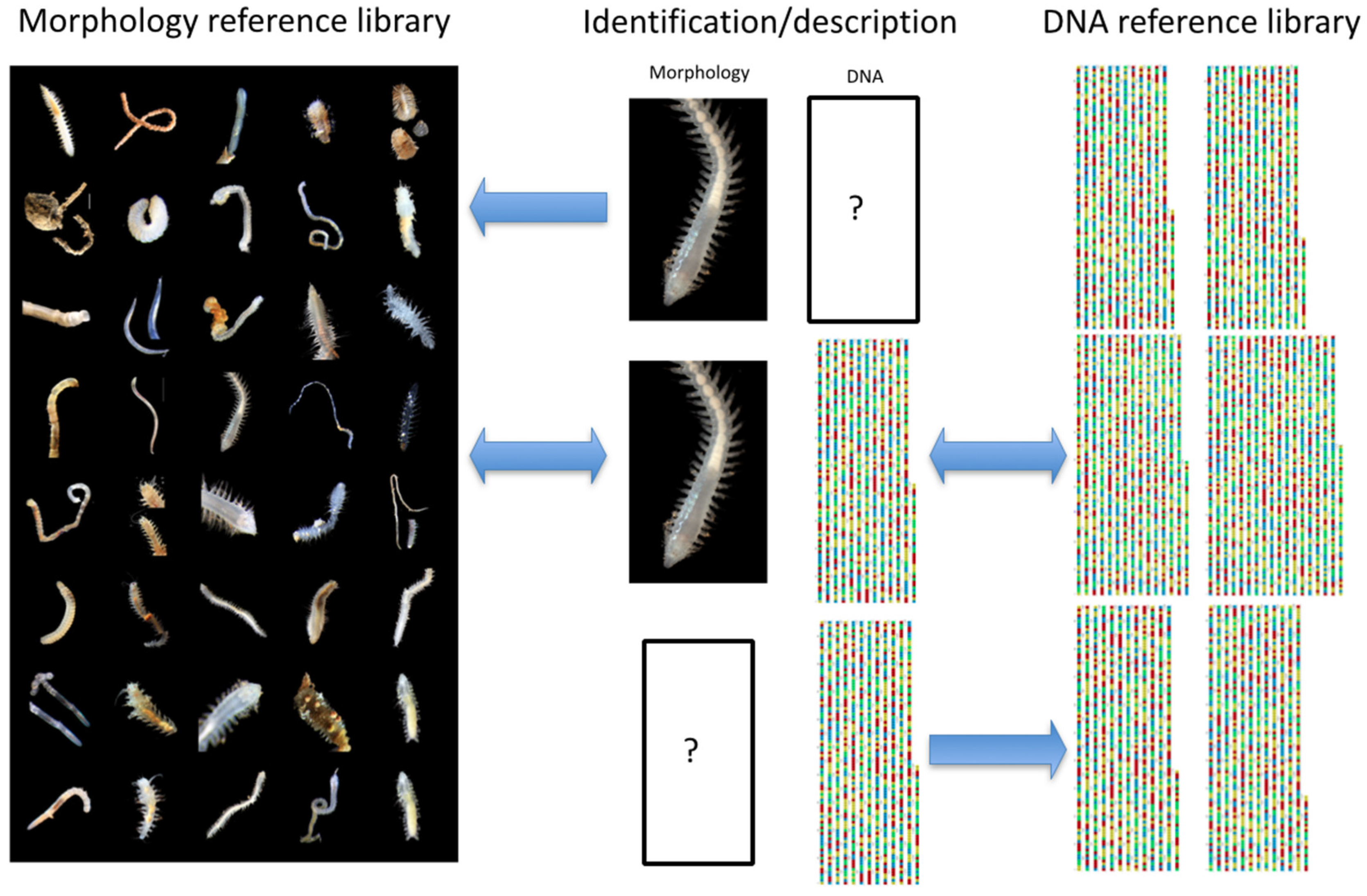
1.1. The Importance of Combined DNA and Morphological Study

A key goal of our sampling protocol for the CCZ is the study of both the DNA sequences and morphology of the animals. Both the genetic sequences of animals, and their external shape and morphology hold huge amounts of useful data for understanding their biology. Over the last 250 years since Linnaeus, humans have been busy building a remarkable and vast reference library to biodiversity based largely on morphology, exemplified in the taxonomic literature, field guides and the collections of museums. Over the past 25 years, a similarly vast reference library has been created that is based largely on DNA or protein sequences, exemplified in online repositories such as the NCBI GenBank (Figure 2). It is obvious that having both genetic and morphological information about species is useful. For example, DNA sequences allow for statistically-rigorous assessment of phylogenetic relationships amongst species; morphological data may provide us with information about a species life-history, ecology, ecosystem function and anatomy.

Figure 2. There are essentially two reference libraries of biodiversity information with regard our planet: one based on over 250 years of Linnean morphological taxonomy (left) and one based on approximately 25 years of DNA and protein sequencing (right). The central panel indicates the problem if only morphology or only DNA is obtained from an unknown organism—the data can only be compared with one library. In order to link both libraries, both kinds of data must be obtained from new species: DNA taxonomy.

Today, an unknown specimen can be DNA sequenced and compared with online databases to identify it. This is what we term “DNA barcoding” or “DNA identification”. However, it only works at species-level if there is an example of the species already sequenced on open databases and linked to a taxonomic name, ideally one that is a described species that is itself linked to voucher or type material in an accessible collection. DNA taxonomy is the creation of that database. In this sense it differs greatly from DNA barcoding: DNA taxonomy is the work that is required to make DNA barcoding possible. It is completely obvious that DNA taxonomy should be undertaken together with morphological descriptions so that when someone identifies a specimen either with morphology or DNA, they have access to both comparative databases (Figure 2).

A version of DNA taxonomy is “turbo taxonomy” or perhaps “express taxonomy” where the DNA data is the primary descriptive and classificatory tool, with the morphology provided as useful additional information that will help field identifications in the type localities, and link the new taxonomy to the traditional taxonomical literature based on morphology only. In fact, a number of recent “turbo taxonomy” papers have included morphological descriptions that are probably at least as good as many standard morphological descriptions from pre-DNA days, e.g., [7]. The “express” part of the taxonomic workflow arises as we can use the DNA evidence as a statistically-rigorous species concept and classification aid, using phylogenetic reconstruction. This obviates the need for difficult and time-consuming comparison of morphological characters about which we have limited knowledge of their usefulness in constructing phylogenies. Key to both types of taxonomy, “turbo” or otherwise, is the data and sample management that must create accessible voucher materials to support species concepts.

Recent years have seen rapid advances in DNA sequencing technical systems, exemplified by the use of, e.g., Illumina machines in what is sometimes termed “next-generation sequencing”. These technologies, developed for the biomedical sciences, are now routinely used in population biology and marine biology DNA studies, e.g., [8,9]. The relative benefits of Illumina (or equivalent) rapid sequencing versus the Sanger sequencing approach are not the subject of this paper. However, it is clear to us that DNA sequencing technology (now very easy) is not the current stumbling block in abyssal biodiversity studies—rather it is the careful collection of suitable samples from these challenging locations using suitable sampling design and sample management. In particular the need for combined DNA (by any method, Illumina or otherwise) and morphology alongside quality taxonomy and sample/data management including the deposition of voucher materials in open collections.

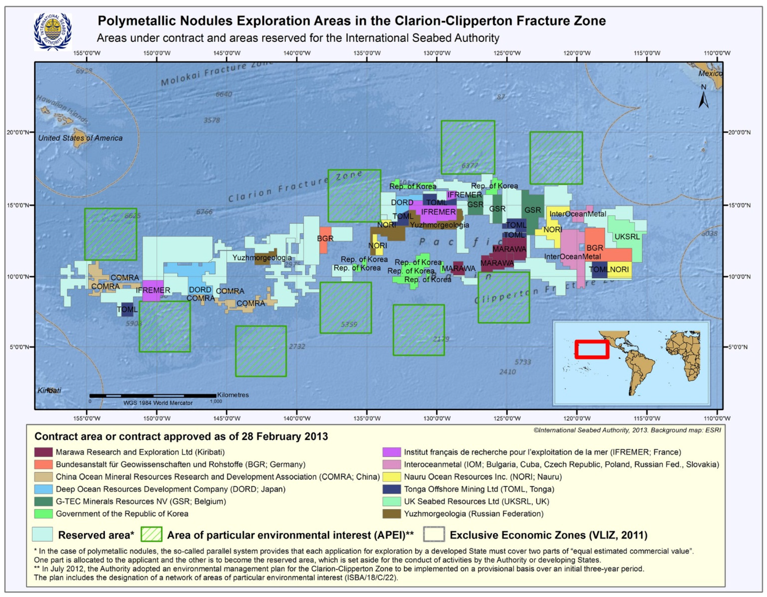
1.2. The Challenges of Zoology in the Clarion-Clipperton Zone

The Clarion-Clipperton Zone (hereafter, CCZ) is so called as it lies between the Clarion and Clipperton Fracture Zones, topographical highs that extend longitudinally across almost the entire Pacific (Figure 1). There is no strict definition of the region, but it has come to be regarded as the area between these fracture zones that lies within international waters and encompasses the main areas of commercial interest for polymetallic nodule mining. Exploration licenses issued by the International Seabed Authority [1] extend from 115° W (the easternmost extent of the UK-1 claim) to approximately 158° W (the westernmost extent of the Chinese COMRA claim), as such we use from hereafter a working definition of the CCZ as the box: 13° N 158° W; 18° N 118° W; 10° N 112° W; 2° N 155° W. This is an area of approximately 6 million sq km, or 1.4% of the ocean’s surface [10].

The vast geographical area of the survey zone is the first challenge. However, the CCZ also encompasses a range of depths (from ~3950 m at the eastern edge to ~5150 m at the western edge), a bathymetric gradient of over ~1200 m. To put this into context, there are significant shifts in diversity and species composition over comparable bathyal depth-ranges from 1500 m to 2500 m that are well documented, e.g., [11]. The simple classification of the entire CCZ as “abyssal” does not necessarily mean that bathymetric trends in species composition will not also be present. The seafloor here is characterized by north-south running more or less smooth hills of approximately 200 m altitude. The CCZ is also punctuated by a large number of known seamounts and/or topographical highs, and a potentially vast number of undiscovered seamounts (Figure 3). These features are likely to influence the local and regional ecology of the seafloor, the sedimentation rates, the strength and direction of seafloor currents and the presence or absence of the polymetallic nodules themselves. Furthermore, the surface water productivity of the CCZ is not uniform. Satellite-derived ocean-color data suggest a general east to west gradient of declining productivity [12], likely to result in a gradient of food availability on the abyssal seafloor [13]. In summary, there should be no pre-conceived hypothesis of zoogeographic homogeneity over such a vast and varied area as the CCZ. As such, high regional biodiversity and species turnover should be hypothesised, and a sampling strategy must be designed with this in mind.

Figure 3. The Clarion-Clipperton Zone (CCZ) is not a homogeneous abyssal plain of mud 4000 m deep. In fact, the depth range of the CCZ is from 3950 m to 5150 m, a range of 1200 m. It is also punctuated by abundant seamounts. Recent expeditions with high-resolution multibeam bathymetry are revealing extremely abundant small seamounts in the eastern CCZ, here illustrated by example from the recent ABYSSal baseLINE ‘ABYSSLINE’ cruise in March 2015. There are 14 definable seamounts typically 200–500 m in height within just one 30 × 30 km sampling strata within the overall 58,000 km² exploration claim. Image credit: Craig R Smith, ABYSSLINE project.

Despite a relatively large number of oceanographic cruises to the CCZ since the early 1970s [2], funded mainly as a result of potential mining interests, there is a complete lack of taxonomic syntheses for the region. As an example, the best current online databases list only 4 polychaete records within a 5° box (300,000 km²) centred on the UK-1 exploration claim area (Figure 4). None of these are records of benthic species, despite polychaetes being the most common macrofaunal benthic animal in the CCZ region, e.g., [14,15]. Even expanding the search box to the entire ~6 million sq km region of the CCZ provides not a single benthic polychaete species record. By comparison, a 5°, 300,000 km² search box centred on the North Sea between the United Kingdom and the Netherlands gives 182,939 polychaete records from 61 datasets (Figure 4) using the Ocean Biogeographic Information System [16]. This discrepancy illustrates the scale of the problem. The region of the North Sea between the Netherlands and the UK is an area of intense industrial activity through fishing, hydrocarbon extraction and the recent growth of offshore wind farms. The environmental regulation of these industries depends heavily on sound baseline biodiversity knowledge, greatly assisted by the availability of taxonomic data and field guides. In contrast, the absence of this kind of data from the CCZ is preventing the sound environmental management of the region by the regulator, the International Seabed Authority, and the sponsoring governments.

Figure 4. Current online databases list only 4 polychaete records from a 300,000 km² search box centred over the UK-1 polymetallic nodule exploration claim area, none of which are benthic species (a); In comparison, the same size search box centred on the North Sea between the Netherlands and the UK lists 182,939 records from 61 datasets (b); Even expanding the search criteria to the entire 6 million km² CCZ produces no published online benthic polychaete records. Data from OBIS [16].

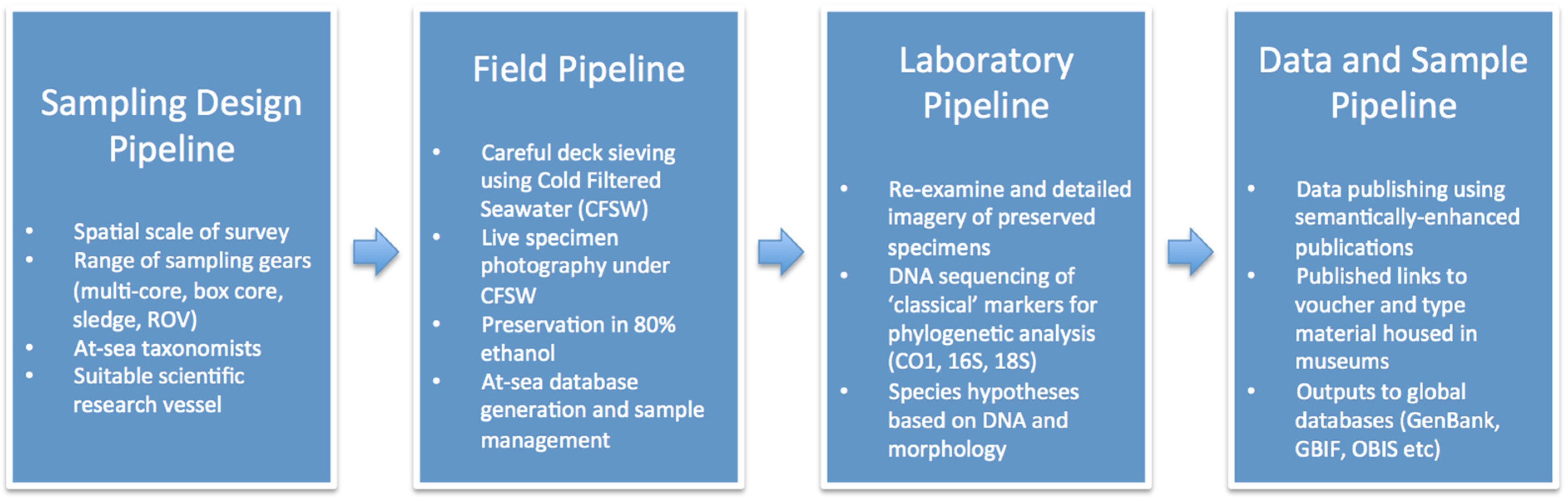
1.3. Methodological Pipelines for DNA Taxonomy in the CCZ

It is clear that consistently reliable methodologies for the DNA taxonomy of species from the CCZ are urgently required given the rapidly-increasing interest in the potential for industrial activity in the area. We present here a series of methodological “pipelines” that we hope will enable researchers and contractors working in the region to work collaboratively to gradually build a modern taxonomic synthesis of the region, upon which environmental impact assessments can be built in the future.

The DNA taxonomy pipeline for the CCZ is a simple methodological workflow (Figure 5) that encompasses the following four key stages:

A sampling design pipeline with consideration to the spatial scale of the required data, the differing biases in sampling gear and the requirement for at-sea taxonomic study
A field pipeline with consideration to the successful collection of high-quality specimens from depths of 4000–5000 m in the central tropical Pacific
A laboratory pipeline with consideration to the needs to collect both DNA sequences and morphological data in a timely and cost-effective manner suited to the immediate needs of the science community
A data and sample management pipeline that includes the publication of results with consideration to the accessibility of data and materials

In the following sections we provide a detailed explanation of the methodology of each pipeline.

Figure 5. We present a methodological pipeline for DNA taxonomy in the Clarion Clipperton Zone that incorporates and end-to-end management approach from the sampling design, field program, laboratory studies and data and sample archiving. This is designed to allow researchers and contractors working in the region to work collaboratively to gradually build a modern taxonomic synthesis of the region, upon which environmental impact assessments can be built in the future.

2. Methodology

2.1. Sampling Design

The goal of the DNA taxonomy method is not the generation of quantitative ecological data, e.g., the numbers of individuals per m² or community composition (itself equally important data, but a different part of a baseline survey), but ideally a list of all the species that live in a sample or ultimately region, with information on those species including their names, phylogenetic position, description and ultimately some data on their natural history such as the presence of reproductive and dispersal characters or observations of feeding. As such, the sampling design must reflect what regional list we want to create. This is not immediately obvious, given that we do not have a particular good a priori understanding of the biogeographic provinces of the abyssal Pacific. For example, it might be that the sampling should constitute all the abyssal areas of the world’s oceans, or just the Pacific abyss, or just the CCZ abyss, or just the eastern CCZ, or just a single exploration claim area.

It is most useful to be guided here by the typical questions that society may ask with regard to the potential for deep-sea mining in the CCZ. Amongst many questions, the ones most relevant to DNA taxonomy are probably: (1) what, and how many, species live in a potentially-impacted area and (2) how widespread are those species outside that area, as such offering them protection from possible extinction?

In a series of discussions and workshops, the Legal and Technical Commission of the ISA has produced a proposed management plan for the CCZ including a series of marine protected areas that surround the CCZ region, called Areas of Particular Environmental Interest (APEIs) [17,18,19]. The APEIs consist of nine 160,000 km² blocks (Figure 1) that are separated from potential mining activities by at least 100 km in any direction, a distance estimated to be sufficient to buffer them from mining impacts [17,18,19]. The mining exploration blocks, none of which have yet been approved for exploitation (given that the exploitation guidelines have not yet been finalised), are also in the general size range of 160,000 km², split between contractor and reserved areas. A typical distance from a mining exploration claim to an APEI is 500–1000 km. Given all this, it is reasonable to assume that a typical scale for which society is likely to expect sound taxonomic baseline coverage, biogeographic data and useful field guides is across sections of the CCZ in the 100–1000 km spatial scale.

The recently-commenced environmental survey of a region of the eastern CCZ, the “ABYSSLINE” (ABYSSal baseLINE) survey, upon which this DNA taxonomy methodology is based, has a sampling design consisting of a series of replicated 30 × 30 km sampling strata within a ~75,000 km² claim area contracted to UK Seabed Resources Ltd. (described in detail in [20,21]). In addition, the project design calls for the sampling of additional sites >1000 km from the exploration claim, for example within the APEI that lies to the north-west of the UK-1 claim area as well as in the central and western CCZ. At the time of writing, 4 sites have been at least partly sampled over two cruises in October 2013 and March 2015, covering scales for DNA taxonomy of 100–1000 km, in keeping with what we expect is a useful and practical scale for the study of benthic biodiversity in the region.

Within sampling strata, the lack of a priori knowledge of the nature of the seafloor or the types or distributions of animals necessitates a randomized sampling strategy, as has been implemented in the ABYSSLINE project (Figure 3). Practical considerations must also be included, for example the presence of hard-substrate seamounts will preclude the use of soft-sediment sampling gears in those areas. Indeed, the range of substrates found in the CCZ is diverse and includes sediment (of varying properties), nodules (of varying sizes and shapes) and seamounts, rocky outcrops and slopes. These different substrates are likely to support different species assemblages all of which we are likely to want to include in our DNA taxonomic studies. For these reasons, for DNA taxonomy of macrofauna and megafauna, we recommend a range of sampling gears that include coring devices, epibenthic sledges (or modified trawls) and in-situ collection using remotely operated vehicle (ROV) or human-occupied vehicle (HOV). Of these gears, only ROV and HOV is realistically suitable for the collection of samples from rocky seamounts and outcrops. Here we describe the strengths and weaknesses of the various sampling gears together with timings and protocols for their deployment in the CCZ at typical depths of 4000 m.

Multiple corer (or megacore). The multiple core, and the more recent modification, the megacore (e.g., the OSIL Bowers and Connelly Mega Core, used in ABYSSLINE), are deep-sea sampling gears that are able to take very precise and undisturbed cores of sediment typically 8–10 cm in diameter and 20–45 cm in length (design and deployment discussed in Barnett et al. [22]). Unfortunately the small sampling area (each 10 cm diameter megacore tube takes only a 31 cm² area of seabed) coupled with the typically low macrofaunal abundances in the CCZ means that these have very limited value for the collection of macrofauna or megafauna. As an example, typical abundances of macrofauna in single megacore tubes on recent ABYSSLINE cruises (to the eastern CCZ, the more productive end of the region) was only in the region of 0–3 specimens per single tube. Even with multiple tubes combined, the volume of sediment is insufficient given the deployment time required for each drop of the gear. However, we describe the protocol here as the megacore can be useful for opportunistic sampling from cores destined for other purposes, e.g., microbiology, and in these cases some rare and very well preserved macrofaunal and megafaunal samples have been recovered from the CCZ using the megacore (Figure 6).

The typical deployment time (from launch off the deck to recovery on deck, not including preparation or deckwork) for a Bowers and Connelly Mega Core (MC) at 4000 m is 3 h 30 min with the following deployment protocol:

Research vessel to hold position using Dynamic Positioning (DP) at location required
MC prepared with 12 core tubes and armed and readied as per manufacturer instructions
MC lifting ring is attached with a swivel to the ship’s trawl wire that is passed through the ship’s starboard A-frame (use of the stern A-frame is not recommended due to pitching)
MC is lifted off the deck with the combination of A-frame and trawl winch, movement is stopped and the securing pin should be set to “armed”
Using the A-frame and the trawl winch, the MC is deployed over the side with swing controlled by soft manila hemp tag lines, which are released when the MC is fully submerged in the water
Wire-out meter is reset with MC at surface, and the MC is then lowered to 50 metres wire out (mwo) and a 12 kHz pinger (1 s time base) is attached to the trawl wire pointing downwards towards the MC
MC is lowered at 40 m/min until 50 metres above bottom (mab), distance from the MC to the seafloor is monitored using combination of the pinger trace on the ships echosounder (e.g., Kongsberg EA 600) and the wire out meter
From 50 mab the MC is lowered at 15 m/min until it reaches the seafloor (visible on the pinger trace) and an additional 10 m wire is then paid out
The winch is then hauled in at 15 m/min until the MC is 50 mab again
The MC is then recovered at 45 m/min
MC is recovered with the assistance of tag-lines attached to poles, and secured on deck ready for processing.

Note that in poor sea states, it is acceptable to go into the seafloor at faster speed of 20 m/min, to reduce the chance of the core bouncing. However, 15 m/min is recommended where possible.

Figure 6. The multiple core (here a megacore type) is not normally a suitable sampling device for the CCZ as the macrofaunal abundances are too low. However, it can be used for opportunistic sampling from cores destined for other purposes—here a primnoid coral on a nodule has been sampled from a core destined for microbiology studies.

USNEL Spade Box Core (or box core). The box core takes a relatively undisturbed 0.25 m² core in soft-sediment or mixed nodule/sediment environments and is an extremely effective sampling device for macrofauna, and occasional megafauna in the CCZ. The box core was first used in the mid 1970s by Hessler and Jumars [23] but has been substantially improved since that time. We currently use a USNEL type 0.25 m² Ocean Instruments BX-S50 MK-III Spade Corer equipped with double hinged top vents to minimize bow-wave effects. The frame on this model is open on one side to allow a dolly-cart to be quickly rolled into position for box-core sample removal. These modifications, which reduce bow-wave effects and allow for quicker sample processing, are highly desirable. In addition, our box-core frame has been modified to accommodate three sets of 24 kg lead weights to prevent the frame from riding up the box core shaft during deployment, helping to limit pre-tripping of the box corer under conditions of heavy ocean swell.

A particular value of the box core in the CCZ region is that the core area is large enough (2500 cm² of sediment per deployment is ~3 times greater than the area sampled by a fully successful meagocore with 12 × 10 cm diameter tubes), allowing efficient use of ship time to collect sediment macrofauna, undisturbed polymetallic nodules, and associated fauna. The nodules can also be carefully removed from the box-core surface with minimal damage to sensitive sessile fauna (see below) (Figure 7).

Figure 7. The Ocean Instruments BX-S50 MK-III Spade Core (BC) (a) is a highly effective sampling device for the CCZ, taking a large enough sample to be useful for macrofaunal studies, as well as a relatively undisturbed collection of polymetallic nodules and the sessile fauna that they support (b); Illustrated is a range of macrofaunal taxa typically less than 1 mm in size collected with box core on the recent ABYSSLINE program to the eastern CCZ (c).

Other equipment required for effective box-core deployments include a deep-sea trawl winch with >½-inch diameter trawl wire, winch speed and wire payout indicators, and a winch tensiometer with graphical display. In addition, a 12-kHz pinger (1 s time base), equipped with cable clamps, and depth recorder with computer display are needed to track the box corer into the seafloor during deployments. Wire tension, wire payout and communications with winch-operator should be available at the depth recorder location in the science lab.

The typical deployment time (from launch off the deck to recovery on deck, not including preparation or deckwork) for a USNEL spade box core (BC) at 4000 m is 5 h with the following deployment protocol, illustrated in Figure 8, and in the Electronic Supplementary Information (Video):

1.

Pre-deployment Preparation

The BX-S50 MK-III BC must be examined and prepared carefully prior to deployment
The spade lifting cable within the BC is easily damaged from normal wear and tear and from marginal sea states; failure of this cable is the most common loss mode of the box corer. The cable should be carefully inspected for damage (e.g., broken or displaced strands) after each deployment, and typically needs to be changed after every 10–15 deployments (Figure 8)

2.

Deployment

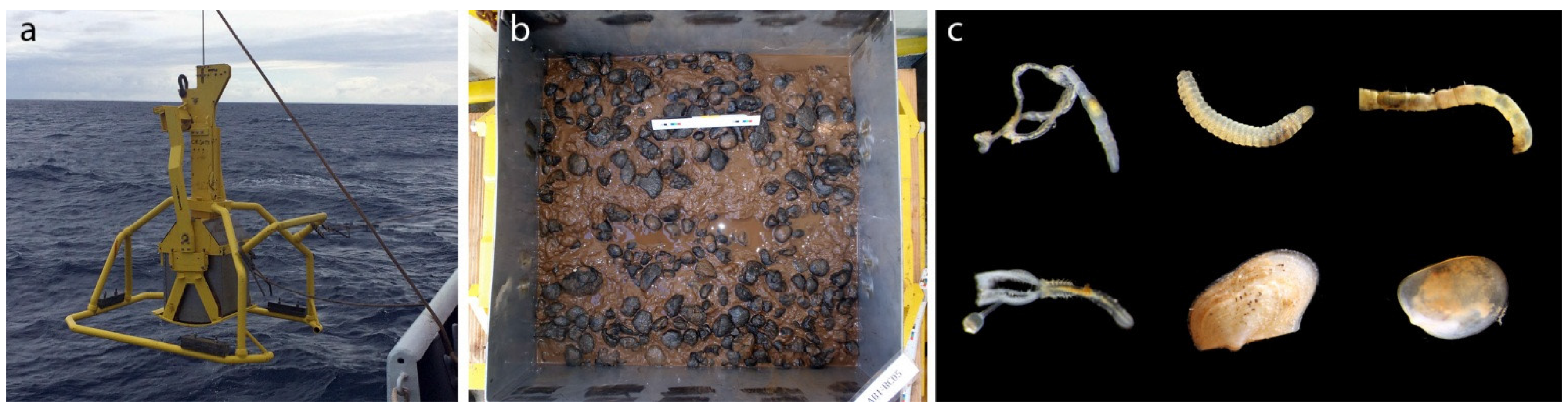
The BC can be moved around the deck on a pallet with pallet jacks, or it can be positioned for deployment using a crane and tag lines. In the open ocean, the BC is ideally deployed from a side A-frame (Figure 8) or crane to reduce the amplitude of ship motion which can cause pre-tripping of the corer; on large vessels (i.e., >75 m LOA), deployment from a side A-frame can dramatically increase box-coring success
The Spade Corer should be attached to the trawl wire with a 3-ton swivel; larger swivels can interfere with firing of the corer
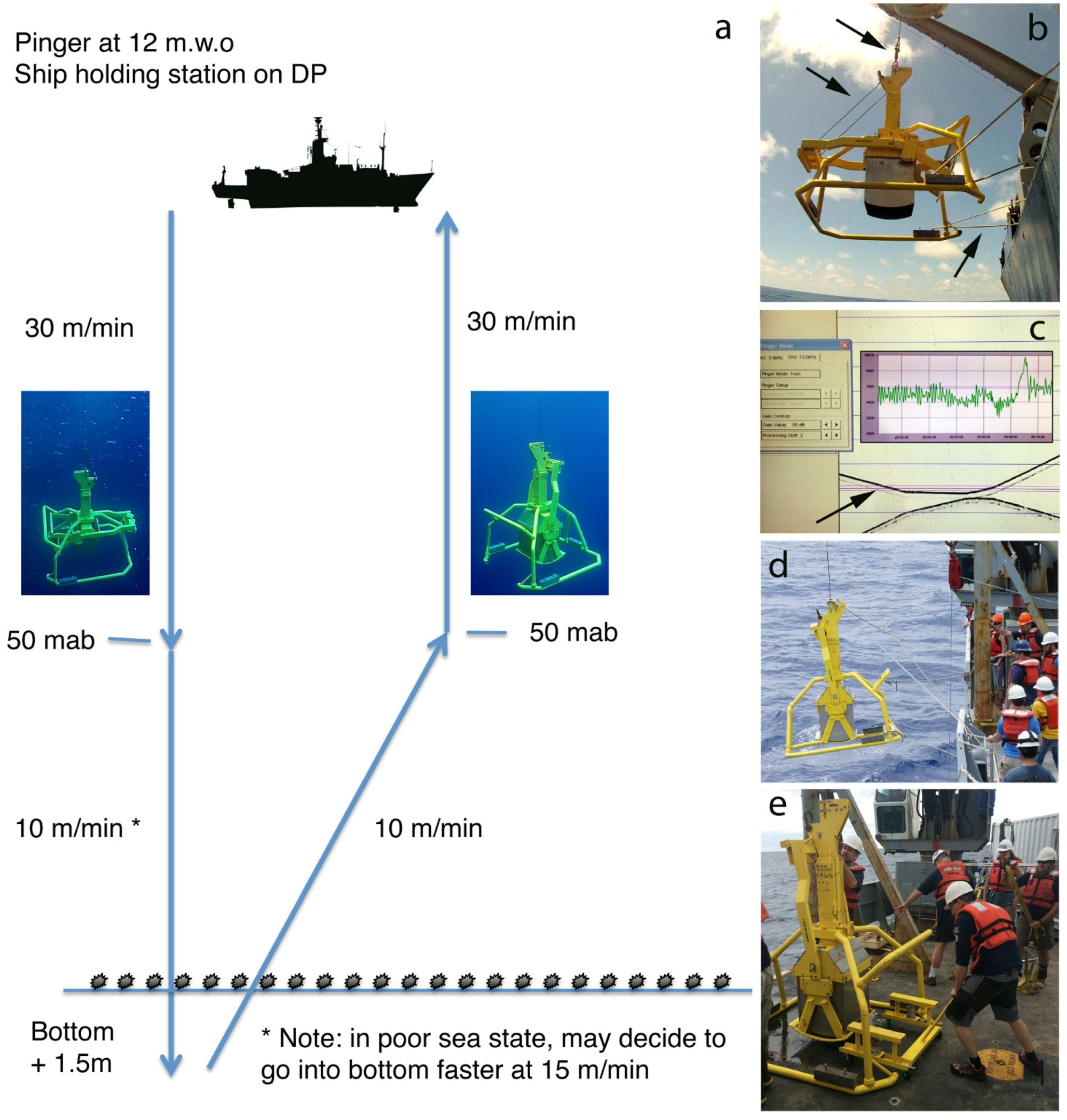
During deployment, the box corer should be controlled by at least three tag lines to restrain swinging of the corer (Figure 8); tag lines should be pulled after the corer has entered the water. Once in the water, the winch payout should be zeroed, and the box corer lowered to 12 m depth. The pinger is then attached to the wire and the box corer lowered at 30 m per minute to within 50 m of the seafloor, while the ship maintains station (preferably with dynamic positioning) (Figure 8)

3.

Control Room and Seafloor Sampling Protocols

Early in the deployment, it is important to check that good traces are received from the pinger, the corer and the bottom. The echo from the corer/pinger and the bottom will cross every 750 m above the bottom with a 1 s interval. On the trace, carefully measure the distance between the corer and the pinger, which will increase by 2 m after coring (Figure 8), or if the corer pre-trips. Check the distance regularly to see if a pre-trip has occurred
When the box corer reaches 50 m above the seafloor, slow the winch speed to 10 m/min and watch the tension plot to observe the normal range in variation before the box core reaches the seafloor. This makes it easier to recognize the drop in tension of about 1000 lbs when the box core reaches the seafloor (note that bottom contact is detectable on the tensiometer before it is visible on the echosounder (Figure 8)). In poor sea states the box core can be put into the seafloor at higher velocities (15–20 m/min) but this typically results in larger bow waves and poorer quality core samples. On the graphical tension display, note when the tension drops ~800–1000 lbs and there is a simultaneous dampening of tension oscillations—this indicates the touchdown of the box corer on the seafloor
Run out an additional 1.5–2.0 meter of wire after touchdown and then stop the winch and immediately haul up at 10 m/min. As the box core is lifted out of the seafloor (after about 3.5–4.0 m of wire have been hauled in) the winch tension will peak and rapidly drop off to background levels. This tension peak is called the “pullout” tension, and reflects closing of the spade and mud suction as the box corer is pulled out the bottom (Figure 8). For successful abyssal box cores, typical pullout tensions are 2500–3500 lbs above background tensions
Immediately following pullout (i.e., the box corer leaving the seafloor) check the distance on the echosounder trace between box corer and the pinger; if the box corer has tripped this distance will have increased by 2 m. (Figure 8) If the box corer has not tripped, it may be set it down again, although trip failures can be caused by set down on a hard bottom. If the distance between the box corer and the pinger has decreased, it is likely that the cable has fouled around the box corer and precaution should be taken during box corer recovery. Once the box core is well off the seafloor, it can be hauled back to the surface at 30 m/min without washing the sample

4.

Recovery

Once the box core has neared ocean surface, tag lines should be attached to the wire below the swivel to limit swinging, and two more attached to the box-corer frame just as it reaches the air-water interface (Figure 8)
Upon recovery, the BC frame must be gently touched to the deck with tension maintained on the cable to prevent to spade from dropping several centimetres and losing the sample topwater; while the box corer is in this position, the dolly-cart should be quickly wheeled under the spade and the carted jacked up to support the spade and box (Figure 8). In addition, the top of the spade arm must be quickly secured to the box-core frame to hold the spade in the vertical position. Once the steps are taken, the sample is secure and can be methodically removed from the box corer (see BC processing protocol, below). The wire tension can also be released and the box corer frame secured to the deck

Epibenthic sledge. The epibenthic sledge (EBS) is a trawled device, variations have been used since the mid 1960s when Hessler and Sanders [24] first used a sledge to record high macrofaunal biodiversity in Atlantic bathyal sediments. An updated version, with 2 collecting nets (the epi-net and the supra-net) and the ability to travel over (rather than dig into) rocky or very soft substrates was developed recently [24]. This is not generally used as a quantitative sampler, as it is very difficult to ascertain the precise area of seabed sampled, or depth of penetration, but it has proved extremely effective in the CCZ for sampling a large number of macrofaunal animals and some megafaunal taxa for taxonomic and biogeographic work. The device is trawled over the seafloor, as the front of the sledge disturbs the sediment/water interface, animals are washed into 2 nets with fine 500 µm mesh cod-ends. Detailed deployment protocols are provided by Brenke et al. [25]. An important modification for work in the CCZ is the presence of an insulated box to enclose the cod-ends (preventing heat damage during transit back to the surface) and a “nodule-excluder” mesh that is positioned at the net openings. This prevents the sledge filling with nodules (Figure 9). Disadvantages of the EBS compared to the box core include the long deployment time and the lack of deep-sediment penetration to collect burrowing infauna which may be missed. On the other hand, the EBS has the advantage (particularly relevant for DNA taxonomy) of collecting over a far broader area and far larger numbers of animals, helping to add rare species to the collection.

Figure 8. Typical Ocean Instruments BX-S50 MK-III Spade Core (BC) deployment protocol. (a) Graphical depiction of the deployment in central Pacific abyssal depths with wire speeds indicated in m/min (mab = metres above bottom). An additional 1.5 m of wire is paid out after BC touchdown. (b) BC being deployed over the starboad a-frame on the RV Melville, 3-tonne swivel (top arrow), lifting cable (middle arrow) and tag lines (bottom) arrowed. (c) Echosounder trace from Kongsberg EA600 software during actual seafloor touchdown of a BC on ABYSSLINE cruises, faint trace from the BC is arrowed, above it is the trace from the pinger with the seafloor reflection rising to meet the BC on touchdown. The slowdown in wire out happens shortly after the arrowed section, after touchdown the distance from the faint BC trace to the pinger has increased slightly (equivalent to 2 m of extra wire out). Inset to (c) shows tensiometer reading, at time point 20:08 oscillation is dampened and the tension rapidly drops, the moment of touchdown, as the BC is then hauled back in the tensiometer rises and the “pullout” as the BC is sucked out of the abyssal mud is clearly visible, indicating a good core has been taken. (d) The recovery team use tag lines to bring the BC safely onto the deck minimising washing of the surface. (e) With the BC lightly resting on the deck (tension maintained on the wire) the dolly-cart is positioned beneath the corer and jacked up to secure the sample—the remaining tension in the wire can then be released and the BC secured on deck.

Figure 9. The epibenthic sledge (a) is a trawled device that is highly effective for the collection of non-quantitative macrofaunal samples with the advantage over the box core of sampling over a wider area. A nodule excluder-grill can be placed over the front of the sledge but small nodules are still retained in the sample (b). (c) Illustration of the typical macrofaunal organisms less than 1 mm in size collected during recent Epibenthic Sledge (EBS) sampling on the ABYSSLINE project to the eastern CCZ.

The typical deployment time (from launch off the deck to recovery on deck, not including preparation or deckwork) for a “Brenke” Epibenthic Sledge (EBS) at 4000 m is 6 h 30 min. For a detailed deployment protocol, readers are referred to Brenke et al. [25] and the deployment is also illustrated in the Electronic Supplementary Information (Video).

Remotely operated vehicle (or submersible). ROVs are now routinely used on deep-sea cruises and recent years have seen several cruises to the CCZ with scientific or commercial ROV. Submersibles are rarely used but offer similar capability to large ROVs. The key goal of ROV sampling from the DNA taxonomy perspective is the collection of large megafauna that are very unlikely to be sampled in box core or EBS. For this reason, it is an essential requirement that the ROV is large enough and modern enough to carry advanced robotic manipulator arms that include suction sampling, high-quality cameras and a range of sampling baskets, normally carried on a tray at the front of the vehicle. Examples of such ROVs in use by the science community are the ROV Jason, ROV Isis and ROV Ropos (Figure 10).

Figure 10. Remotely operated vehicles (ROVs) (a) are essential to the successful collection of high-quality megafaunal samples (animals several cm or larger and rarely caught in box core or EBS). They also permit in-situ observations of organism behaviour and appearance prior to collection. (b) Large ROVs are needed that incorporate manipulator arms which can be used to collect CCZ organisms such as holothurians (c). Image credit (c) Craig R Smith and Diva Amon, ABYSSLINE program.

Deployment times and protocols for ROV work vary greatly depending on the device used. With enough technical support crew, an ROV like Jason or Isis can work 24 h a day, with recovery to the surface only needed to unload samples, move the ship at speed or undertake maintenance. The use of free-vehicle elevators can alleviate the need to recover the ROV for samples, this can be particularly useful in CCZ work where a large number of replicate scoop or push-core samples may be needed.

ROVs can be equipped with a wide variety of sampling gears each with their own individual requirements. Most useful in the CCZ habitat are simple scoop nets for recovering megafauna (e.g., sea cucumbers) and suction samplers. Small push cores are a feature of most modern science ROVs but these are unlikely to be of use for macrofauna or megafauna in the CCZ, but have potential for meiofaunal or microbiological sampling—although a mega core sample can also perform this function.

In summary, the most important sampling gears for DNA taxonomy in the CCZ are the box core, the EBS and the ROV. None of these gears on their own is sufficient, as they are each complementary in their collecting biases. Traditional trawls such as the Aggasiz Trawl have not so far been used with great success in the CCZ owing to the presence of nodules. In addition, not considered here are highly motile fauna, such as fish or scavenging crustacea which are present on the CCZ benthos and almost impossible to capture with ROV. A portion of the fish fauna can be collected via baited traps, the challenges of this are discussed elsewhere, e.g., [26].

2.2. Field Pipeline

Here we describe a series of at-sea protocols that will help enable other researchers to collect high-quality macrofaunal and megafaunal samples from the CCZ benthos for DNA taxonomy using a “cold-chain” that maintains low temperatures for organisms from the moment the sample comes on deck until preservation in ethanol. We assume here that the sampling gears are deployed according to the standard protocols (referred to above) and secured on deck. At-sea protocols are also illustrated in the Electronic Supplementary Information (Video).

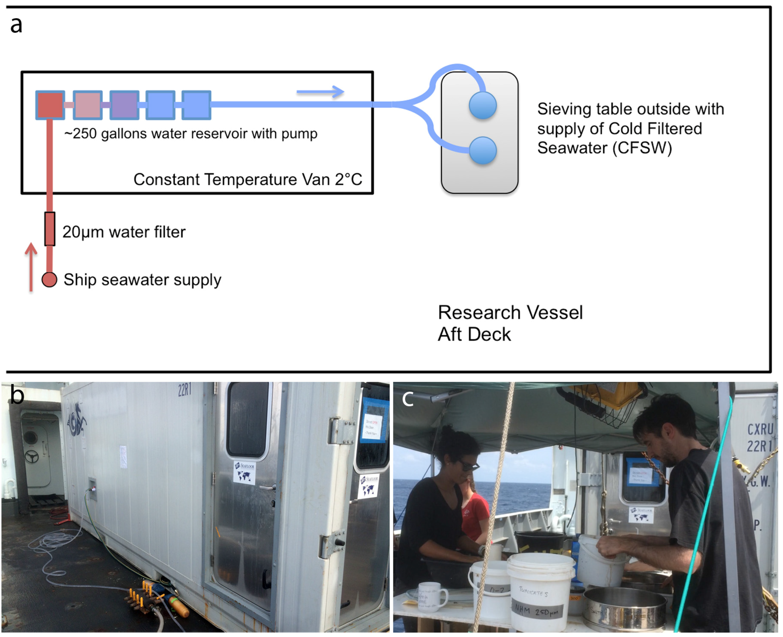
2.2.1. Cold Filtered Seawater (CFSW) System Protocol

The purpose of this protocol is to setup a system that will allow a regular supply of cold, filtered seawater on the deck or in the lab to allow processing of samples. There are two basic approaches, the one below or the purchase of a large, industrial seawater chiller unit. The latter has not yet proved to be reliable and is relatively expensive. Typical surface water temperatures of 28 °C in the CCZ (compared to seafloor temperatures of ~2 °C) make the chilling of seawater a challenge. However this is essential to DNA extraction success from small animals.

Protocol CFSW—equipment required

Pumped seawater supply system from the ship (this may claim to be filtered, but almost always requires additional filtration as detailed below). Note that these systems are standard on oceanographic research vessels
A large constant temperature (CT) van or room that can be set to 5 °C or lower (ideally 2 °C) with easy access to the back deck. The chilling system or van needs to be robust and of high quality to enable operations in high humidity, high temperature for months at sea. This system is not standard on oceanographic vessels and must be hired or purchased
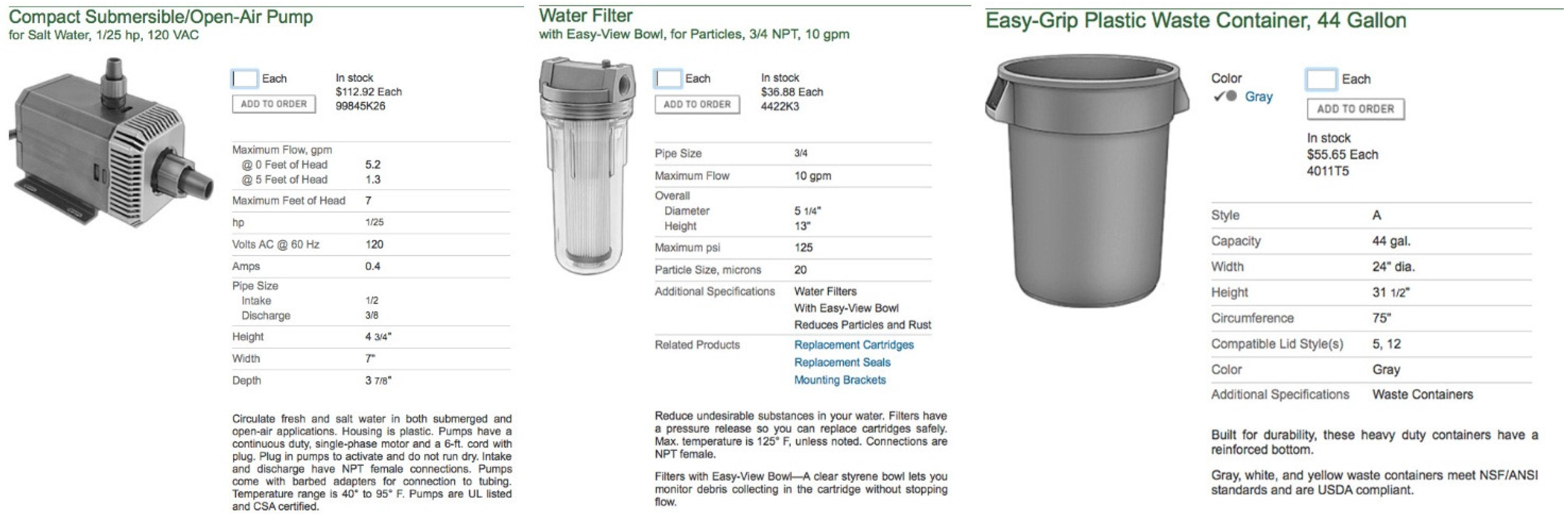
Water reservoir of as large a volume as can be achieved, ideally something in the region of 750–1000 litres (200–300 US gallons). A low-cost option is 5 × 170 litre (44 US gallon) plastic trash cans, these need to be secured carefully in the CT room in case of ship movement. An alternative is high-quality water storage reservoirs built into the CT lab that can be plumbed in and connected together using a flow-through system.
At least 3 saltwater submersible pumps with approx 1/25 hp rating (Figure 11)
Garden hose connectable water filter system (20 µm rating) with replaceable cartridges
~50 m of garden hose
~15 m of clear soft 12 mm (½ inch) “tygon tube” type plastic hose
Misc hose connectors to connect filters and pumps to hoses, including adaptor from the ship’s outlet to the garden hose
Some flow control valves and “Y” splitter valves to put in various places (e.g., at end of hose near sieve, next to filters, etc.).
2–3 large plastic trays 10–20 cm deep approx 80 × 50 cm that will fit the sieves and if you are sorting in a lab, fit in the sink (see processing protocol)
Most items can be purchased in any good large hardware store (Figure 11)

Figure 11. Three essential pieces of equipment for setting up a low-cost cold-filtered seawater system on a research vessel are submersible pumps (a), water filter (b) and simple water storage containers (c). These are installed in a constant temperature van or room on the back deck (Figure 12), which must also be rented or purchased. Images from http://www.mcmaster.com.

Figure 12. Typical cold filtered seawater (CFSW) setup on ABYSSLINE cruises. (a) Diagram showing the location of a constant temperature (CT) van on the back deck, with inflow of seawater from the ships pump (typically not filtered and at surface temperature of ~28 °C) into a filter, then a series of water containers in the cold room, then via controlled hoses back out of the van onto a sieving table (b,c). A system like this can store about 1000 litres of CFSW and provide water to sort 2–3 box cores over a 24 h period.

Protocol—CFSW setup (Figure 12)

Install 5 × 170 litre (44 gallon) drums, or similar water storage system (e.g., flow-through connected drums) in the CT room or CT van, secured
Connect ship seawater system to water filter on deck, and run from filter with garden hose into the CT room, with flow valves inside to control flow into the drums
Install a salt-water submersible pump in the CT room tanks, with control switch inside CT room
Run 12 mm (½ inch) tygon (clear plastic hose) from submersible pumps back out of the CT room onto the deck, with Y-splitter and control valves as required
Typical usage to process 1 box core is 190–380 litres (50–100 gallons) of CFSW
Typical time to chill 190 litres (50 gallons) surface water from the CCZ at 28 °C in a 2 °C CT room to ~4 °C is 4 h

The CFSW protocol does not allow for continued 24-h processing of box cores (or similar samples) and on a typical oceanographic cruise in the CCZ, box core sampling would be spread amongst other activities. Typically this protocol would be sufficient for 2–3 box cores to be taken in a 24 h period, which is more than would typically happen given that the typical deployment time for a box core at 4000 m is 5 h.

2.2.2. Box Core Processing Protocol (for DNA Taxonomy)

It is important to note here that the majority of box core samples on ABYSSLINE cruises, and on most other cruises we are aware of, are used for quantitative community ecology analysis. The protocols for these studies are not described here, but in essence the goal is the very careful collection of all the macrofaunal organisms living within a core to establish data on abundance and community structure, e.g., [23]. Typically these samples are quite large, and are preserved in formalin, which is unsuitable for DNA study.

The goals of DNA taxonomy are slightly different, as is the processing, but with careful control of the sample it is possible to achieve both quality DNA taxonomy and quantitative ecological study from the same sample. The most important rule to follow to achieve this is that no part of the mud sample must be thrown away except that which has passed through a 300 µm sieve (see note below on sieve sizes), and that all organisms picked for taxonomic study must be tracked so that the numbers can be fed back into the quantitative ecological study.

This is achieved in the ABYSSLINE CCZ stations by taking careful samples of all the nodule fauna, and taking sub-samples of the sediment for DNA taxonomy. Data on the numbers of each taxon taken for DNA taxonomy, and their identity is returned to the quantitative ecology group.

Typically, we recommend that box core processing is done on an outside deck, next to the supply of CFSW, with a shade setup to protect the box core from the tropical sun (Figure 13). In some instances depending on the ship, it may be possible to process the box core inside a lab or hangar, but it is important to note that the volumes of mud produced are very large (hundreds of litres of muddy water per box core).

Figure 13. Processing mud samples from box core and EBS on deck. (a) Siphoning off the top-water from the box core onto 300 µm sieves; (b) Removing remaining surface water with a syringe/baster; (c) Picking large megafaunal and macrofaunal animals to a chilled CFSW container; (d) Picking nodules and rinsing them to remove mud prior to examination under microscope; (e) Cutting the box core (here a sub-sample for live-sorting for DNA taxonomy) prior to sieving; (f) Sieving mud from the box core in a submerged sieve under CFSW; (g) Picking the remaining heavy fraction of an EBS sample for small bivalves. These process are also illustrated in the Electronic Supplementary Information (Video).

Time is of the essence when processing box cores as the core heats up quickly, damaging organisms and their DNA. Tight organisation of the sorting team (typically 4–5 people) is required.

It is useful to comment here briefly on the sieve sizes. Recent ISA workshops have discussed a proposal that for quantitative study, a 250 µm washing sieve may be more appropriate than a 300 µm sieve for the quantitative sorting of CCZ box cores [27]. However, the typical definition of “macrofauna” in the deep sea is animals that are retained on a 300 µm (or in some cases 500 µm) sieve. We are also not aware of any studies that support the proposed 250 µm classification. Hence on the recent March 2015 ABYSSLINE cruise we undertook quantitative sampling using nested 250 µm and 300 µm sieves in order to retain the 250–300 µm fraction separarately and to investigate the utility of the 250–300 µm fraction for macrofaunal studies in the CCZ. The quantitative investigation of these data are ongoing, but it was immediately noticed that there were very few macrofaunal animals in this fraction (based on initial observation and sorting only) and this small fraction of the sample contained a relatively large volume of sediment, in particular radiolarian ooze, making microscope sorting extremely time-consuming and difficult for the relatively few animals recovered. Although a fully quantitative investigation is needed, for the purposes of DNA taxonomy at least we do not recommend the use of a 250 µm sieve size. For observation of our box core protocol, we recommend the Electronic Supplementary Information (Video).

Protocol—box core processing—equipment required

Supply of CFSW from cold van, 5–6 wash bottles pre-filled with CFSW
Plastic 20 litre buckets labelled 0–2 cm, 2–5 cm, 5–10 cm, each pre-filled 1/3 with CFSW
3–4 plastic trays for nodules
300 µm sieve (2) with deep trays to hold sieves inside
Short (1.5 m) lengths of vinyl hose for siphoning water from top of box core
Large syringe or turkey basters for siphoning water from top of box core
Forceps and small dishes/trays for megafauna to be collected immediately
Trowels for cutting mud
Camera, flashlight, thermometer

Protocol—box core processing—preparation

Once box core is secured on deck, with cart underneath and ready to be moved:

Examine box core surface with flashlight
Measure top water temperature (make note)
With two tubes, drain some of the surface water through 300 µm sieve but without disturbing top layer
Roll box core out on trolley (slowly) and secure on deck in shade.
Drain remaining top water through 300 µm sieve and use turkey basters or syringes, etc., for remainder of the water
Photograph exposed surface with label

Protocol—box core processing—nodule and megafauna sampling

Pick obvious unattached megafauna to place in small CFSW buckets/dishes on ice
Remove nodules carefully, rinse each nodule in the 0–2 cm bucket and with CFSW wash bottles
Place nodules onto a nodule-storing foam tray or egg tray from galley, keeping them upright → tray to lab (keep cool)

Protocol—box core processing—mud sampling

Remove sub-section (depending on amount of sample to live sort) of 0–2 cm for DNA taxonomy/live sorting, place into 0–2 cm CFSW bucket and store in cold van
Repeat with 2–5 cm and 5–10 cm sections
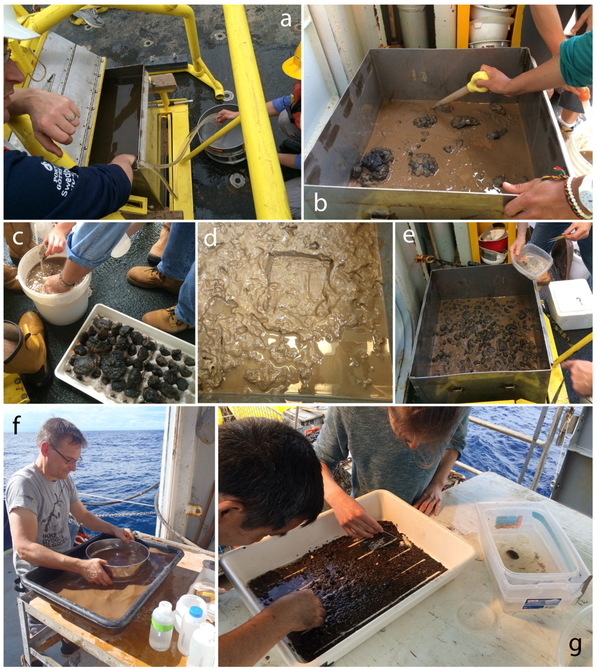
Sieve samples with 2 people, 1 to hold sieve and 1 person to pour water and collect sample
Gently agitate buckets of mud and pour slowly onto sieve, keeping sieve underwater in tray (Figure 13)
Tap sieve gently from underneath to help material go through sieve if necessary
Regularly wash material (with wash bottle) retained on the sieve to a small beaker, as soon as material is in this dish store in the lab (fridge) for live sorting/DNA taxonomy

Note that multiple cores (or megacores) can be processed in essentially the same way, although in the CCZ the numbers of macrofaunal organisms from the megacore is likely to be too low to be useful.

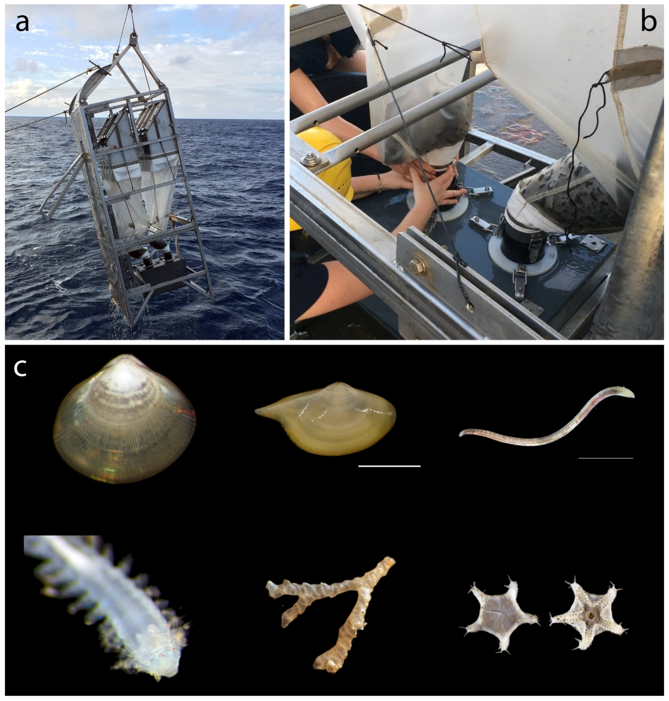
2.2.3. Epibenthic Sledge (EBS) or Trawl Processing Protocol

The general principle is the same as for BC, but usually there is less mud, and many more nodules (Figure 10), since small nodules enter the nets through the nodule excluder grid. Nodules are likely to be scraped against one another in the net, hence the nodule fauna is likely to be damaged, so the collection of nodule fauna is a lower priority. The CCZ version of the Brenke EBS contains a “nodule excluder” which results in only small nodules being collected.

Large megafauna that can be picked from net or cod end should be processed individually as below (large megafauna protocol).

The protocol here assumes the EBS is on deck and secured.

Protocol—EBS processing—equipment required

Supply of CFSW from cold van, 5–6 wash bottles pre-filled with CFSW
~1 m wide 50 litre tubs labelled “epi” and “supra” net for the two cod-end samples from the EBS
3–4 plastic trays for nodules
300 µm sieve (2) with deep trays to hold sieves inside
Forceps and small dishes/trays for megafauna to be collected immediately

Protocol—EBS processing—processing for DNA taxonomy

Once sample is secured on deck:

Remove cod-ends into CFSW “epi” and “supra” buckets (rinse cod-ends with CFSW from hose)
Wash material on nets into buckets (with CFSW)
Remove remaining nodules to large buckets
Photograph sample
Pick megafaunal animals into CFSW trays or small dishes -> transfer to lab for DNA taxonomy
Sieve EBS mud/cod-end sample with submerged 300 µm sieve in CFSW as for box core processing (Figure 13), transfer sample to small beakers to take to lab for DNA taxonomy/live sorting
Pick through remaining large “gravel” fraction using white trays outside (Figure 13)

2.2.4. Large Megafauna Processing Protocol (e.g., ROV, HOV or Trawl Collected)

The principle is similar to that for the box core and EBS samples: keep samples cold, obtain high quality imagery and take samples for DNA and morphology taxonomy. Larger samples can have a small sub-sample taken in 80% ethanol for DNA with the remainder preserved in 10% formalin. It is important to have time to make observations with regard reproductive features, commensal and parasitic organisms.

Protocol—Large megafauna processing—equipment required

Supply of CFSW from cold van, 2–3 wash bottles pre-filled with CFSW
Selection of small and large buckets pre-filled with CFSW to receive ROV samples
300 µm sieve (2) with deep trays to hold sieves inside
Forceps and small dishes/trays for megafauna to be collected immediately

Protocol—Large megafauna processing—processing

Collect specimens by hand from ROV or HOV bioboxes/storage trays
Maintain specimens in buckets or trays of CFSW and remove to lab for live sorting
Wash remaining biobox water through 300 µm sieves (as with EBS protocol) to collect smaller fauna and associated fauna

2.2.5. Live Sorting for DNA Taxonomy Protocol

Once the samples are secured and in cold storage operations can be moved from deck to lab, bringing samples out (one by one) from the fridge or cold room into the normal lab for microscopy, sorting, imaging and fixation. Ideally this can happen right away if some people can work on the deck and some in the lab. Live sorting of specimens at sea removes the problem of contamination (e.g., with surface water samples, or mixing of benthic samples), which is relevant to ongoing investigations of the utility of environmental (eDNA) approaches to identifying fauna [28]. We do not currently believe eDNA methods are particularly useful for identification of CCZ macrofauna until a quality reference library of identified, sequenced material has been created, based on carefully sorted material (the goal of our methodology).

The same live sorting protocol applies to all samples from box core, EBS or ROV. The only differences are that the sorting times are much longer for EBS samples as the volumes of sample are much higher. It can typically take 5–6 h to live-sort one EBS cod-end sample with 3 people helping. For the most part, careful sorting and processing of the nodules is only significant with the box core samples, as those collected by EBS are heavily washed and damaged.

An extremely important principle is that the lab work must be undertaken even if samples are backing up on the deck. This can happen in the CCZ when long periods of good weather can allow a large number of repeated samples. For DNA taxonomy, it is more important to have 10 well-preserved individual animals, photographed, sampled for DNA and tissue stored in the freezer than 10 jars of unsorted mud in which the DNA and morphology of animals has degraded. With this in mind, we highly recommend that the sampling program spaces apart sampling efforts to allow the biologists undertaking DNA taxonomy sufficient time between samples to allow processing.

An essential part of the protocol is the maintenance of cold temperatures for the samples throughout from the removal from the fridge, to the live sorting until they are fixed in 80% ethanol. Although some research vessels have constant temperature laboratories (e.g., set to 4 °C) it is not recommended to live-sort in these conditions given the long hours that are required and the physical stress to the sorters. Instead, it is possible to maintain the cold-chain in a normal lab environment through careful preparation and planning as detailed here. This is also illustrated in the Electronic Supplementary Information (Video).

Protocol—Live sorting for DNA taxonomy—equipment required

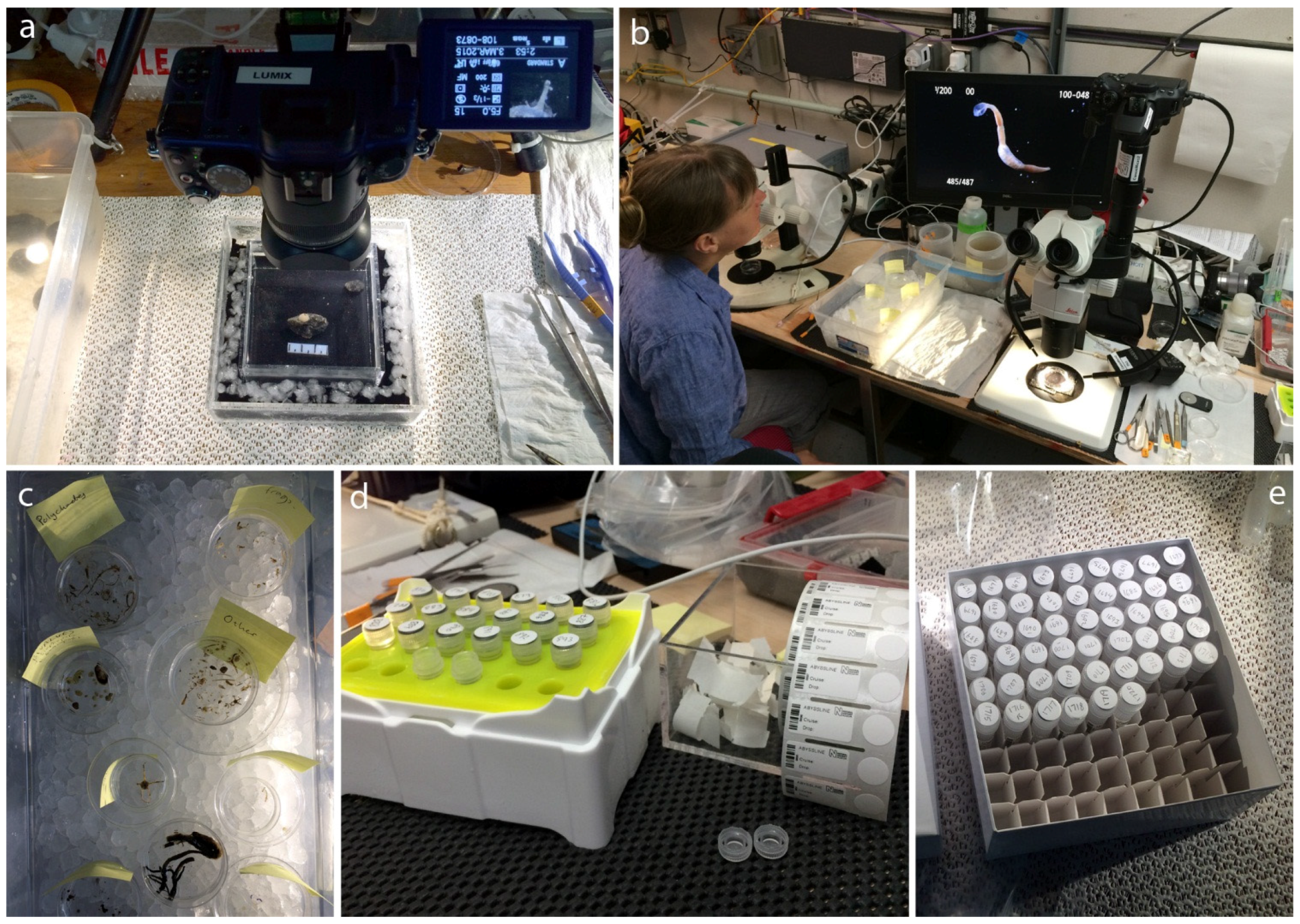
~6 m of laboratory bench space inside a comfortable research vessel general purpose lab with chairs suited to microscope work (Figure 14)
Easy access fridge for temporary live-sample storage, and −20 °C freezer for storage of preserved specimens
Machine for crushed ice (not ice cubes)
2× high-quality stereomicroscopes (e.g., Leica MZ9.5 or equivalent) equipped with photography tube
2× high-quality DSLR cameras attached to microscopes (e.g., Canon 700D or equivalent) together with 4× strobe (flashguns) equipped with eTTL and wireless (slave) mode (e.g., Canon 430EXII or equivalent)
2× full HD 1080p screens to output HDMI live view from the DSLR cameras
2× high-power fibre optic light sources (e.g., Leica CLS150 or equivalent)
1× macro-photography suite consisting of table tripod, DSLR camera with 45 mm (90 mm in 35 mm equivalent) macro lens, light source (flexible fibre optic work lamps that clamp to bench, low cost and effective is IKEA “Tived” LED clamp light article 701.696.94)
Acrylic trays for photography and ice baths (Figure 14)
General laboratory sorting consumables including 2 ml, 20 mL and 50 mL plastic microtubes (e.g., Sarstedt), plastic pipettes, dissection kits, wash bottles of CFSW, tube racks (including low-temperature gel pack tube racks), labels for jars (Figure 14)
Compact desktop computer (e.g., Mac Mini) for storing sample database and images from cameras
Supply of 80% ethanol in wash bottles, kept chilled. This needs to be non-denatured ethanol that is diluted to 80% with laboratory DI water (not tapwater or seawater). It is important that the ethanol used is 80% absolute ethanol (non-denatured) in 20% DI water, not pure 100% ethanol as this greatly reduces the dehydration and physical damage to the specimens, allowing them to be used for good quality morphological study as well as DNA. As the ethanol is only used in the final storage of the specimens in the microtube vials, the amount of ethanol required equates to the number of final vials stored. As a guideline, on the recent March 2015 ABYSSLINE cruise to the CCZ (a 42 day cruise using a range of sampling gear) we used ~1500 2 mL microtubes and ~100 20 mL vials a volume of ethanol equal to 5 liters (although only macrofauna and DNA tissue samples from large animals were taken). We would recommend taking 2× the amount of ethanol calculated and consumables on top of that anticipated, and in particular if large megafauna are to be fixed intact then obviously larger quantities are needed, or large megafauna (20 cm long holothurians, etc.) can be fixed in low-cost 10% buffered formalin using standard methods with just a small tissue sample (e.g., body wall, muscle) taken for DNA.

Figure 14. Live sorting at sea for DNA taxonomy in the Clarion Clipperton Zone. (a) Polymetallic nodule with sessile macrofauna imaged live while kept cool on ice using macro-photography suite; (b) Typical photomicroscope setup showing sorting tray (with ice), camera system with HD viewing screen showing live image, wet black cloths under petri dishes to create black backgrounds, strobe lighting to improve resolution and dissecting tools; (c) Typical live sorting of an EBS sample into class prior to imaging and preservation; (d) Low-temperature micro-tube rack (insulated) for storing vials, each given barcoded labels and unique specimen number; (e) Specimens transferred into storage boxes prior to being placed in −20 °C freezer and shipment to laboratory at end of cruise. This process is also illustrated in the Electronic Supplementary Information (Video).

Protocol—Live sorting for DNA taxonomy—large fauna and large CCZ nodule fauna

Larger animals (megafauna 1 cm in size or greater) and nodule fauna are normally collected by ROV or from collection from the surface of the box core. A typical box core sample from the CCZ will contain several species of sessile nodule fauna (excluding meiofauna and foraminifera) which need to be treated with this protocol. It is important to record all macrofaunal and megafaunal nodule fauna to add to the quantitative ecological dataset being collected by the ecology team.

It is here assumed that specimens have been brought in from deck and are being kept in the fridge in CFSW.

Place the specimen (or nodule) into a clean CFSW water bath (using acrylic trays) fully submerged with a wet black cloth under the tray to create a black background. This can be achieved by placing 1 bath inside another, with ice surrounding the internal bath (Figure 14).
Photograph the specimen or nodule with macro-lens DSLR held in tripod with good lighting (powerful LED lights are sufficient, strobe not required unless the specimen is moving) on black background with scale bar.
For nodule fauna, remove individual specimens after photography and if necessary image under the photomicroscope camera for higher-resolution.
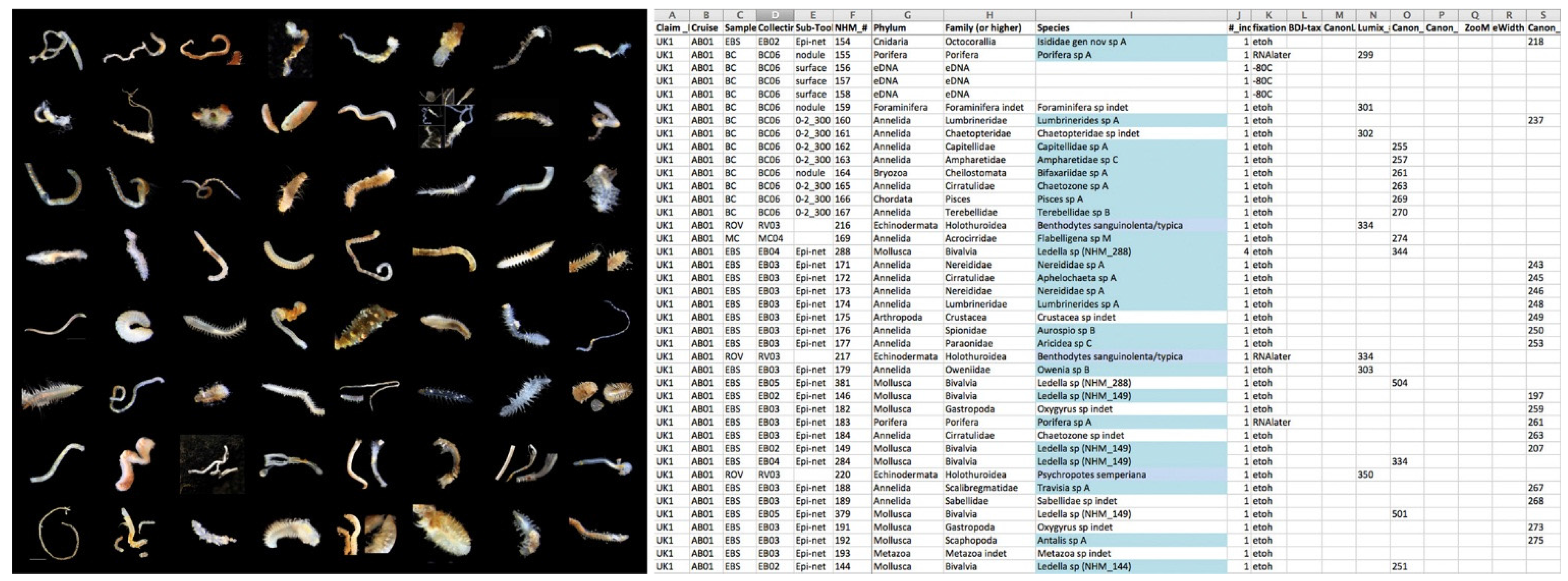
Using the spreadsheet database, assign a specimen number and add a record of the camera photograph number (normally the best one). Make sure the spreadsheet has enough columns to cover various different cameras. Add any other relevant data (gear, station, preliminary identification, notes, etc.).
For very large specimens (e.g., big sponges) remove a small piece of tissue and place in vial labelled with the specimen number. Add chilled 80% ethanol and store in chilled tube racks. Remainder of specimen can be fixed in formalin or ethanol in a large jar with the same specimen number.
For small specimens the whole animal can go in a microtube vial (normally 2 mL or 20 mL in size for CCZ organisms). Label and top up with chilled 80% ethanol.
Store all samples on chilled tube racks (Figure 14), once samples have built up they can be transferred to labelled microtube boxes and stored in −20 °C (Figure 14).
All data recorded to an on-the-fly lab live sorting spreadsheet (Figure 15).
Depending on fixed use, some samples may be fixed in RNAlater (e.g., for metagenomic eDNA studies) or −80 °C freezer.

Figure 15. The expected end result of successful live sorting for DNA taxonomy in the CCZ. (a) An example image database here of 60 different annelid species imaged live; (b) On-the-fly database creation with end-of-cruise data (typically list of specimens identified to class/family and sometimes genus).

Protocol—Live sorting for DNA taxonomy—BC and EBS sieved samples

It is recommended that two people are assigned to this task if possible. Typically, one person can be handling the nodules and large fauna, a second person sorting (picking) animals from the sieved residues. Once the residues are picked, both people can then help with the photography, fixation and database work.

Small aliquots of the sieved residues are transferred to petri dishes with CFSW. The petri dishes are then sorted under the microscope using standard picking methods. The petri dishes can be kept cool by placing them on pre-chilled microscope bases (kept in freezer) or pre-chilled, wet black cloths
Picked animals are sorted initially into major taxon under the microscope (bivalves, polychaetes, etc.) and kept in small petri dishes on ice (Figure 14)
Once the sort is complete, the residues for the box core sample (i.e., sorted waste) is returned to the quantitative box core sample. Unwanted EBS sample can be discarded or bulk-fixed
Specimens can be cleaned by transferring to new petri dishes and fresh CFSW, for photography.
Specimens are photographed using the photomicroscope and strobes (Figure 14)
Specimens are transferred to 2 mL microtubes with 80% ethanol and kept chilled, data is added to the spreadsheet as for the large/nodule fauna protocol above
Photographic tips. A clean specimen in clean CFSW on a new petri dish, the dish supported on a wet black cloth (under the dish) helps to achieve a high-resolution image with black background (Figure 15). Periodically wetting the black cloth with chilled seawater also helps to keep the specimen cool
Photographic tips. Specimens should be imaged using two strobes in wireless (slave mode) with the image taken using a remote switch (to avoid vibration). Typically, white balance should be carefully adjusted to conform to the strobe lighting, and the exposure compensation function used to prevent over-exposure of any part of the specimen. Patience is required to achieve good photographs

The end result of the field pipeline is a database of specimens identified to typically family or better resolution, each specimen imaged several times in high-resolution and stored in −20 °C 80% ethanol ready for shipment to institutional laboratory (Figure 15).

Protocol—Live sorting for DNA taxonomy—Shipping samples

At the end of long oceanographic research cruises, there is much concern and effort put into the shipping of samples. For mixed DNA/morphology taxonomic work (excluding RNA work) there is no need to ship samples frozen. Individual specimens that are picked from the mud and preserved in 80% molecular-grade ethanol can be shipped at room temperature for up to 1 week with no noticeable decline in preservation standard. Our recommendation is that specimens are shipped by standard air-freight in 80% ethanol in small quantities following the guidelines of the shipper.

2.3. Laboratory Pipeline

The goal of the laboratory pipeline is to build upon the data and materials collected at sea to create species hypotheses based on phylogenetic evidence supported by morphological data and accessible voucher or type materials. These species hypotheses then form the basis of the DNA taxonomy publications (Section 2.4).

The methods for sequencing of markers such as COI, 18S, 28S and 16S are well described elsewhere in the scientific literature, and we only briefly describe our methods here as relevant to work in the CCZ, alongside our table of primers used (Table 1).

Protocol—Laboratory imaging and sampling

On return from the ship, specimens can be kept in the microtubes they were sampled in and in a normal laboratory fridge (−20 °C freezing is not required).

All specimens are re-examined using high-power microscopy and imaged for morphological features (e.g., polychaete chaetae) (Figure 16)
A small tissue sample is taken for DNA sequencing, this can be an individual polychaete parapodia, antenna or slice of body wall. A simple rule is that if the tissue sample is visible to the naked eye it is big enough for DNA sequencing. A typical minimum we use is a piece of tissue of 0.5 mm × 0.5 mm, roughly the size of the end of a fine pencil
Remainder of the specimen is kept for morphological study or further DNA sampling if required
Species hypotheses are created later based on DNA phylogenetics (not before)

Figure 16. Laboratory pipeline for DNA taxonomy on return to institution (here Natural History Museum, London). (a) Second set of imaging of important morphological characters (here a polychaete chaetae); (b) DNA prep lab in the Darwin Centre; (c) Robotic workstation for automated DNA extraction and sequencing; (d) PCR machine.

Protocol—DNA extraction and sequencing

These are based on well-established protocols but with some modifications for CCZ fauna:

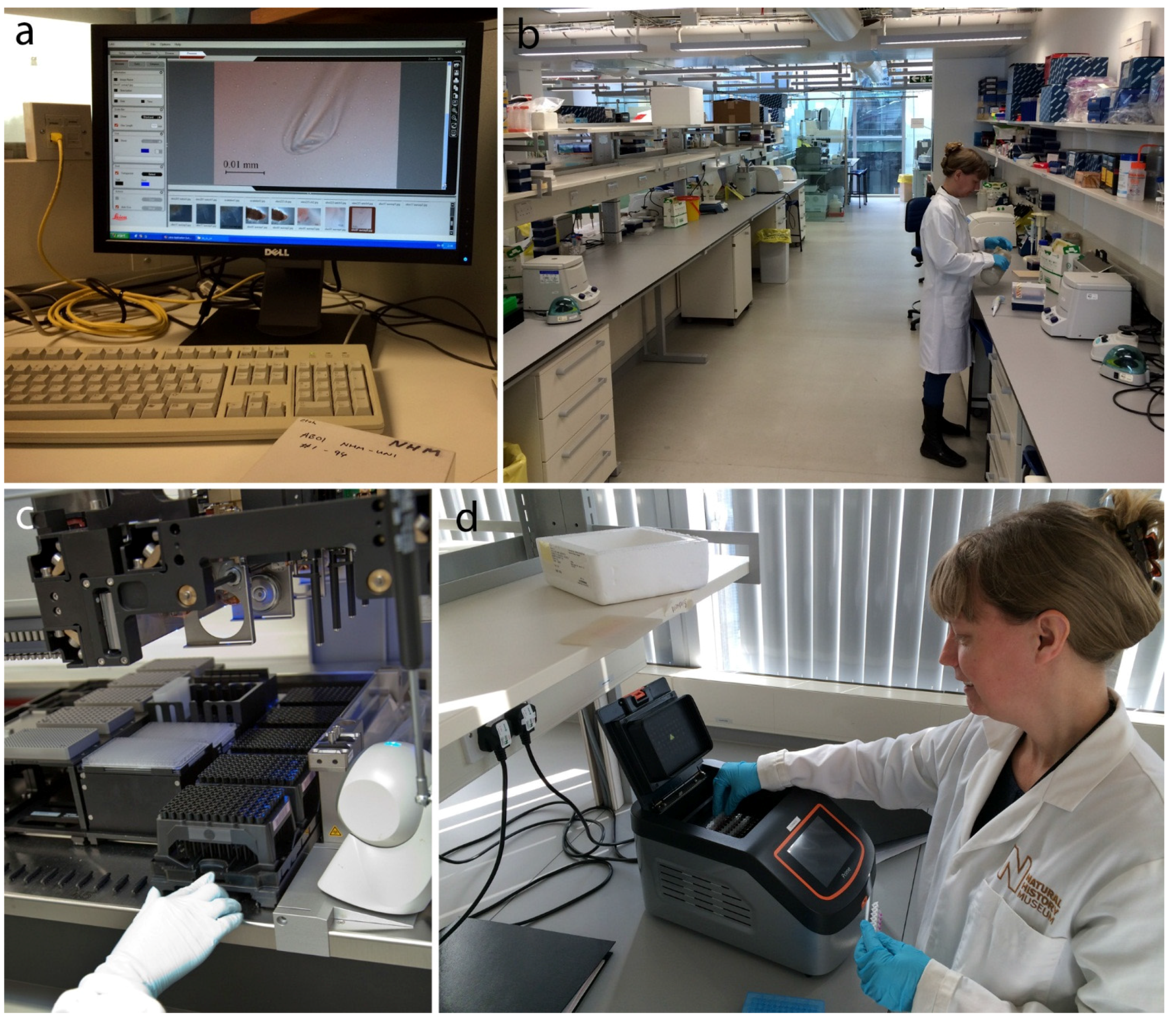
Extraction of DNA is undertaken using DNeasy Blood and Tissue Kit (Qiagen) using a Hamilton Microlab STAR Robotic Workstation (Figure 16)
Typically, about 1800 bp of 18S, 800 bp of 28S (D1-D2 region), 450 bp of 16S, and 650 bp of cytochrome c oxidase subunit I (COI) are amplified using either published or newly-designed primers (depending on the taxa of choice). Primer pair combination for 16S that is working on most CCZ phyla is Ann16SF together with 16SbrH. Furthermore, the COI primers originally designed for polychaetes, polyLCO-polyHCO (Table 1), works well on a range of other phyla, e.g., Bryozoa, Cnidaria, Echinodermata, Mollusca and Chordata
Typically, PCR mixtures contain 1 µL of each primer (10 µM), 2 µL template DNA and 21 µL of Red Taq DNA Polymerase 1.1× MasterMix (VWR) in a mixture of total 25 µL. The PCR amplification profile consists of initial denaturation at 95 °C for 5 min, 35 cycles of denaturation at 94 °C for 45 s, annealing at 55 °C for 45 s, extension at 72 °C for 2 min, and a final extension at 72 °C for 10 min
Typically, PCR products were purified using Millipore Multiscreen 96-well PCR Purification System, and sequencing was performed on an ABI 3730XL DNA Analyser (Applied Biosystems) at Sequencing Facility, using the same primers as in the PCR reactions plus two internal primers for 18S

Protocol—DNA analysis

Overlapping sequence fragments are merged into consensus sequences using Geneious [29] and aligned using MAFFT [30] for 18S, 28S and 16S, and MUSCLE [31] for COI, both programs used as plugins in Geneious, with default settings
Bayesian phylogenetic analyses (BA) are conducted with MrBayes 3.1.2 [32] following standard methods for phylogenetic inference

Table 1. Primers used for PCR and sequencing of all benthic CCZ mega- and macrofauna phyla except crustaceans.

**Table 1.** Primers used for PCR and sequencing of all benthic CCZ mega- and macrofauna phyla except crustaceans.
Primer	Sequence 5′-3′	Reference
18S
18SA	AYCTGGTTGATCCTGCCAGT	[33]
18SB	ACCTTGTTACGACTTTTACTTCCTC	[34]
620F	TAAAGYTGYTGCAGTTAAA	[34]
1324R	CGGCCATGCACCACC	[35]
28S (D1-D2)
C1′	ACCCGCTGAATTTAAGCAT	[36]
D2	AACTCTCTCMTTCARAGTTC	[36]
COI
LCO1490	GGTCAACAAATCATAAAGATATTGG	[37]
HCO2198	TAAACTTCAGGGTGACCAAAAAATCA	[37]
COI-E	TATACTTCTGGGTGTCCGAAGAATCA	[38]
polyLCO	GAYTATWTTCAACAAATCATAAAGATATTGG	[39]
polyHCO	TAMACTTCWGGGTGACCAAARAATCA	[39]
16S
16SarL	CGCCTGTTTATCAAAAACAT	[40]
16SbrH	CCGGTCTGAACTCAGATCACGT	[40]
Ann16SF	GCGGTATCCTGACCGTRCWAAGGTA	[41]
Ann16SR	TCCTAAGCCAACATCGAGGTGCCAA	[41]

Protocol—Combined DNA and morphological species hypothesis

The phylogenetic trees produced are used to identify consistent monophyletic clades of specimens and derive phylogenetic species concepts (sensu Donoghue, Nygren and De Queiroz [42,43,44])
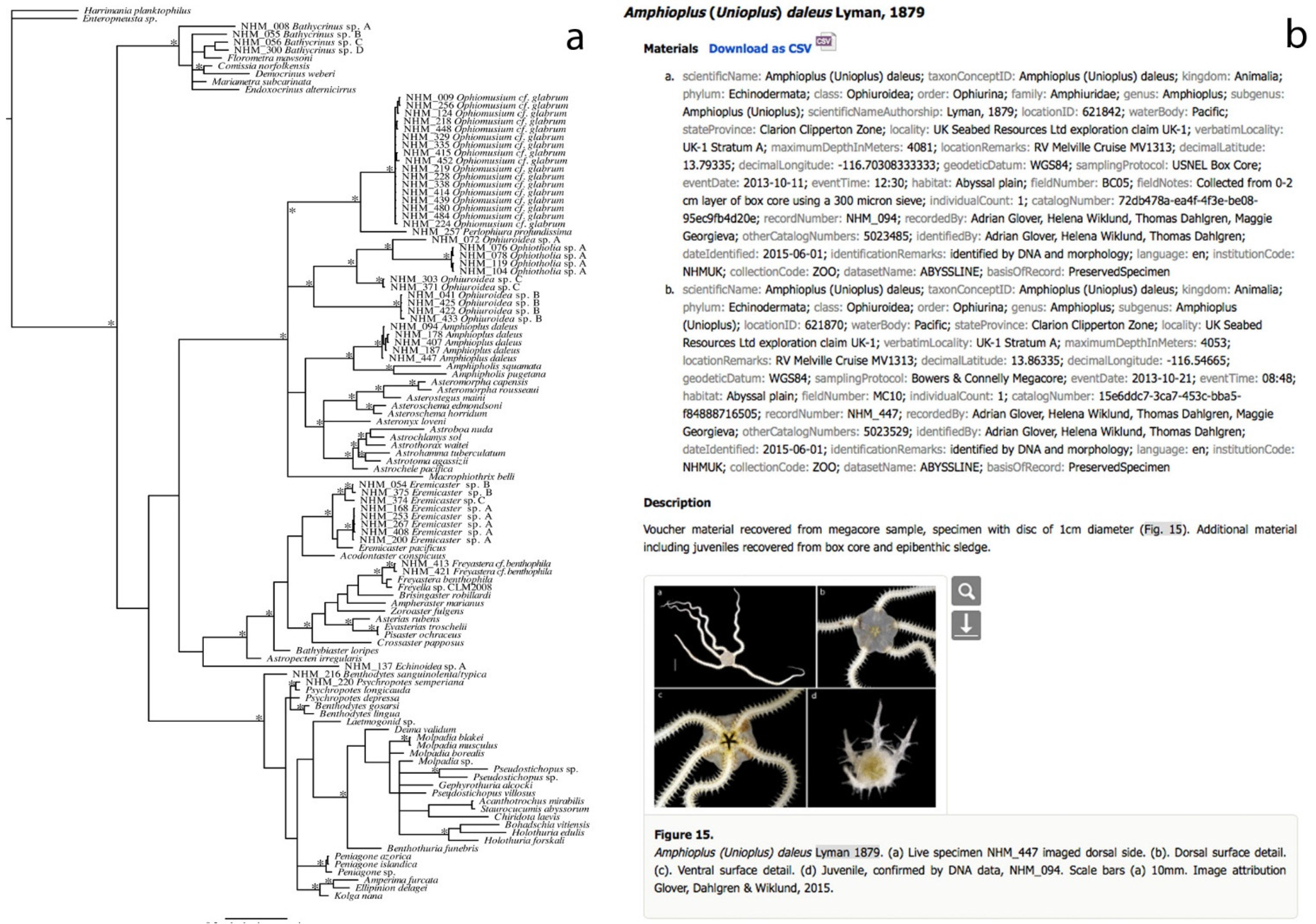
Statistically well-supported clades where “within-clade” sequence variation is lower than “between-clade” variation are hypothesised as species (Figure 17)
Morphological data is condensed for each species concept, and a type, series of types or voucher allocated
Taxonomic species descriptions or records based primarily on genetic data supported by morphological information to aid identification in the field are produced in a taxonomic data paper format (Figure 17)
Site and associated data are organised into the bioinformatics-standard Darwin Core (DwC) [45] format to support online publication and data management (Figure 17 and see Section 2.4)

Figure 17. Abyssal plain DNA Taxonomy. (a) Phylogenetic analysis is used to generate statistically-supported species hypothesis (here by example a working tree for echinoderms from the CCZ). (b) Taxonomic species descriptions or records based primarily on genetic data supported by morphological information to aid identification in the field are produced in a taxonomic data paper format supported by site data organised into Darwin Core (DwC) format ready for upload to online databases such as OBIS.

The end result of the laboratory pipeline is the creation of publication-ready taxonomic data manuscripts that incorporate combined DNA and morphological data. An example is provided in Glover et al. [46], dealing with the DNA taxonomy of echinoderms from the CCZ.

2.4. Data and Sample Management Pipeline

Data and sample management is of critical importance to both the scientific validity and long-term value of the taxonomic data produced in the field and laboratory pipelines. With this in mind, as an example, we describe here the data and sample management pipeline being developed for the ABYSSLINE DNA taxonomy program.

Recent years have seen a revolution in the availability of online biodiversity data, led by data systems such as NCBI Genbank [47], the Global Biodiversity Information Facility [48], the World Register of Marine Species [49] and the Ocean Biogeographic Information System [16]. Whilst these systems have some overlap in terms of their data content, they have in fact evolved quite separate niche spaces and are highly complementary. For example, although WoRMS contains species occurrence data, it is primarily a taxonomic list of names maintained by a network of taxonomic editors—as such it feeds a highly-updated taxonomic database to systems that use it such as OBIS and GBIF.

A primary goal of the protocol described here is the output of high-quality taxonomic data to these open-access data systems supported by a peer-reviewed taxonomic data publication. Recently, publication systems have been developed that allow for the publication of biological “data papers” in a semantically-rich online format that allows instant availability of data on supported web systems, such as GBIF. These have major advantages over traditional (PDF or print) publication in that the data within the papers is directly searchable and readable by online systems [50]. This is exemplified by the use of “Darwin Core” format for species occurrence data, a standardized data format that ensures data is available to online systems that are compatible, such as GBIF and OBIS.

Protocol—Data and sample management

The protocol described here, is a series of connected workflows that are highly interlinked and to some degree dependent on the institutional data management systems (Figure 18). We describe here the protocol for the ABYSSLINE DNA taxonomy project which is likely to be compatible with most institutional/museum data systems:

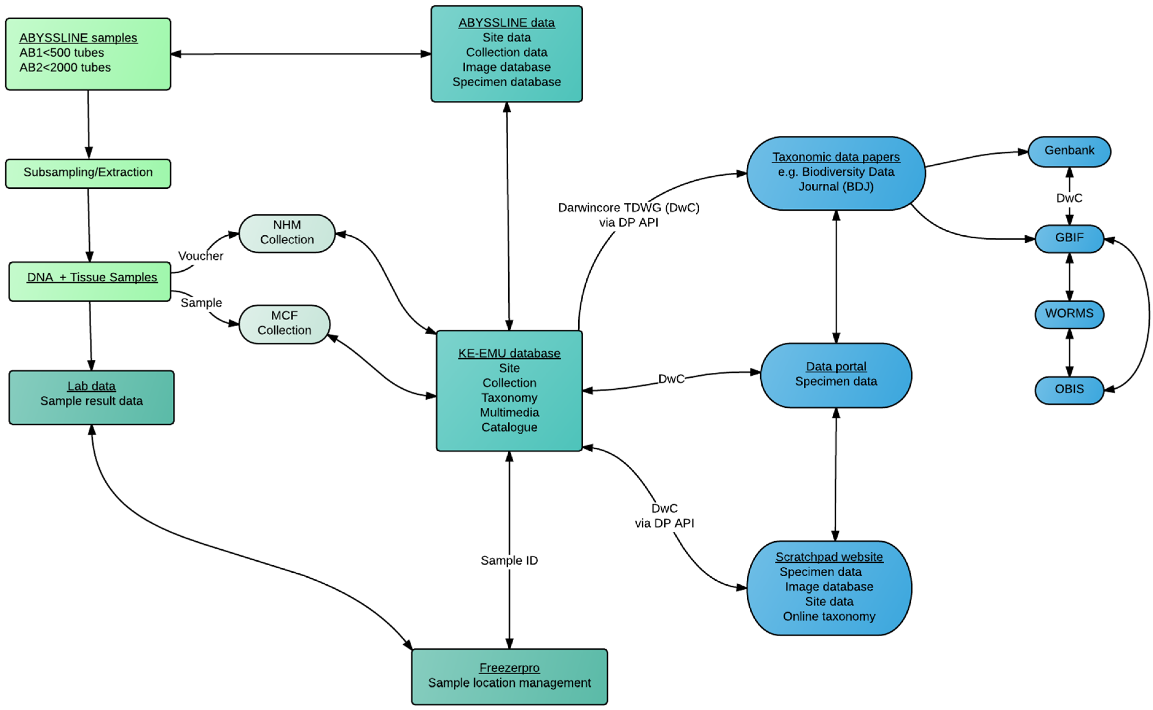
The data and sample products from the field and laboratory pipelines (which can reach many thousands of physical objects and data points—e.g., Figure 18) are fed into institutional-level databases, in the case of ABYSSLINE this is the KE-EMU database (a central NHM database) and the FreezerPro database (a database for all frozen tissue samples in the Molecular Collection Facility (MCF) of the NHM)
The central institutional databases are used to create Darwin Core (DwC [37]) outputs of species occurrences and site data to feed into institutional public-facing sites that include the NHM Data Portal [51] and Scratchpads [52]
The DwC outputs are also linked to the taxonomic data papers, in most cases using semantically-enhanced publications such as Biodiversity Data Journal [50]
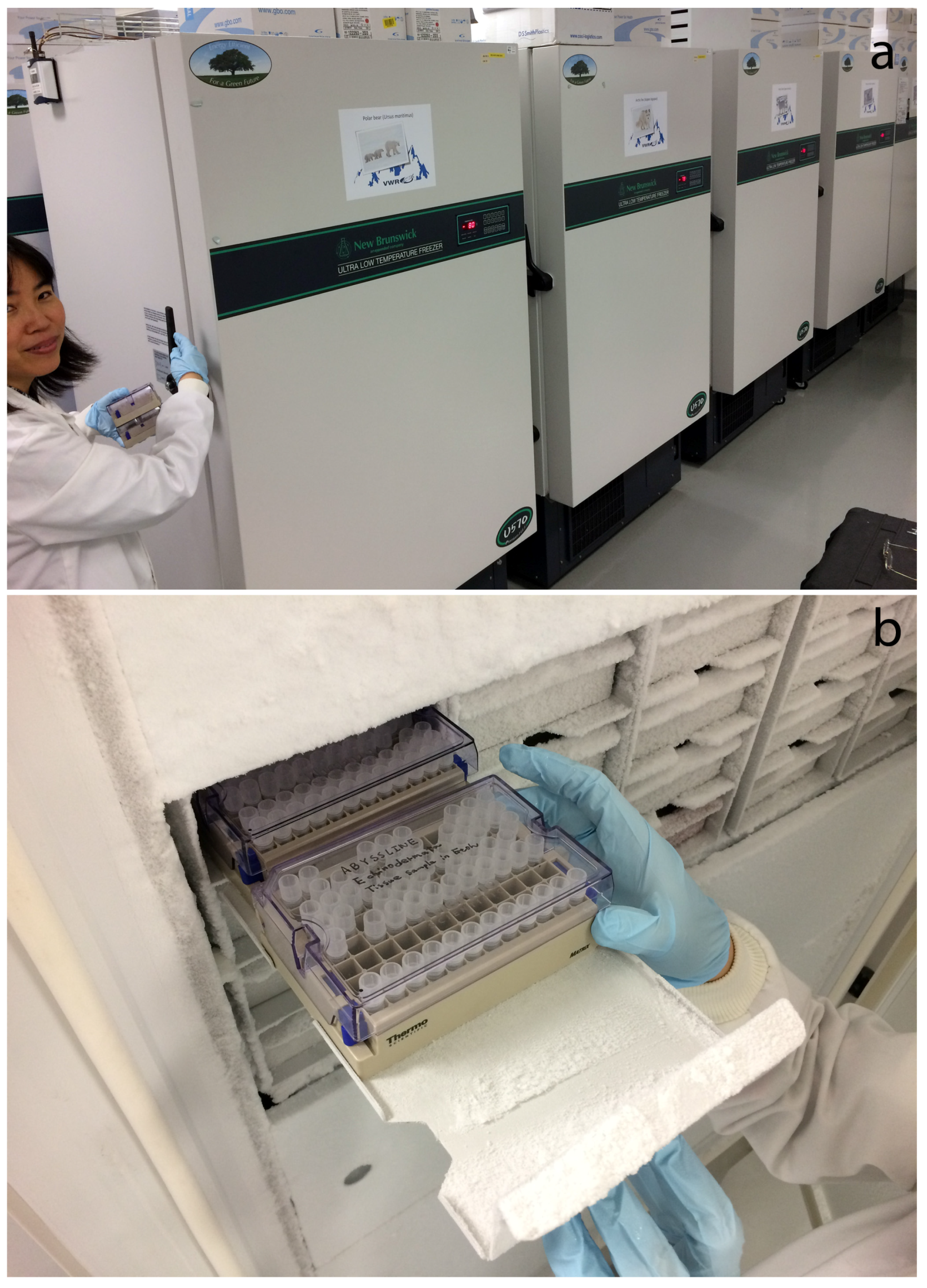
The physical samples are stored in two long-term collections—the NHM national collection for ethanol-fixed specimens and the NHM Molecular Collection Facility where tissue samples and DNA template is stored at −80 °C freezers with backup power systems. These samples are maintained by the NHM curatorial staff, and accessible to researchers (Figure 19)
The DwC outputs from the taxonomic data papers (e.g., Biodiversity Data Journal) are automatically made available to external databases including GBIF and OBIS, with DNA sequences available on GenBank
DwC outputs can also be used for a project-level (multiple institution) public-facing or project website to enhance collaboration and data sharing amongst project members during the project phase, implemented in the Scratchpad
All external use of the data or samples is linked to the peer-reviewed data paper which allow data users a stable DOI citation to use as well as contact details for the authors, and associated data

Figure 18. Data and sample management workflow on the ABYSSLINE DNA taxonomy project. Physical research-lab based samples are represented by light green boxes, physical institutionally-accessioned samples by grey ovals, institutional data by dark green boxes and externally-available data by blue ovals.

Figure 19. The final resting place for ABYSSLINE tissue and DNA extract samples in the data pipeline is the −80 °C freezers of the Natural History Museum Molecular Collection Facility. This is a curated facility with multiple freezers connected to backup power systems and emergency notifications of power failures designed for the long-term storage (and ability for researchers to sample) DNA and tissue samples. Here two plates containing echinoderm tissue sample and template DNA are loaded into the freezer “Polar Bear”.

3. Discussion and Conclusions

The ultimate goal of our methodological pipeline is to publish quality taxonomic data from the CCZ abyss to support sound governance and environmental management of the region. The pipeline describes how to do this in such a way that in future years, given funding for the work to be undertaken, an online search will we hope reveal a large number of species records from the area, linked to online publications, genetic data and samples that are all accessible completely independently of the original researchers that created them. This ensures long-term viability of the data and the iterative building of biological knowledge of the CCZ. It will also ultimately allow us to create useful field guides to this part of the ocean, an essential step forward in our baseline biodiversity knowledge.

There is a considerable cost involved to the generation of these data, and it is vital that contractors and regulators look carefully at the costs of an environmental baseline survey beyond just the sampling cruise itself. The first large-scale oceanographic expedition (the Challenger expedition), which commenced almost 150 years ago, took 4 years to complete, but 19 years for the publication of results and dissemination of data and samples into accessible museum collections. The accessibility of those materials means that they are still examined and worked on today. In areas such as the CCZ, modern biologists need to return not to the methods, but to the fundamental principles that were used in those early expeditions to ensure the long-term usefulness of their science.

Supplementary Materials

A video file “Glover & Dahlgren 2015 Clarion-Clipperton Zone DNA Taxonomy” highlighting key aspects of the field methodology is available as supplement to this paper and at https://youtu.be/Io7NlFKUmYI.

Acknowledgments

The ABYSSLINE environmental survey is supported by a collaborative partnership between 6 non-profit global academic research institutes (University of Hawaii, Natural History Museum, Uni Research, National Oceanography Centre, Senckenberg Institute, IRIS Norway) and through a commercial arrangement with UK Seabed Resources Ltd. We acknowledge the support of all of the scientists of the ABYSSLINE project. We are particularly grateful to Magdalena Georgieva, Madeleine Brasier (NHM), Diva Amon, Iris Altamira (University of Hawaii) for their time on the cruise assisting the NHM/UNI team with all aspects of the sampling and photography. We would particularly like to acknowledge the outstanding support of the crew and technical support staff of the survey vessels RV Thomas G Thompson and RV Melville where the methods were tested on recent cruises. In addition we would like to thank Muriel Rabone, Chiho Ikebe and Jackie Mackenzie-Dodds in the Molecular Collections Facility, Natural History Museum (assistance with data and sample management, and Figure 18 and Figure 19), James Horsfall (assistance with cruise de-mobilization and the “end-to-end” terminology) and Harry Rousham (contract administration, NHM). Where faces appear in the figures, permission has been granted by those that appear.

Author Contributions

Ideas and practical experiments with different methods were conceived and carried out by all the authors. The manuscript was drafted by A.G.G. and subsequently discussed and commented by all the authors.

Conflicts of Interest

The authors declare no conflict of interest. The funders had no role in study design, data collection and analysis, decision to publish, or preparation of the manuscript.

References

International Seabed Authority Home Page. Available online: http://www.isa.org.jm (accessed on 14 December 2015).
Nimmo, M.; Morgan, C.; Banning, D. Clarion-Clipperton Zone Project, Pacific Ocean: Updated NI 43–101 Technical Report; 127631013–003-R-Rev1; Golder Associates Pty Ltd.: Milton, Australia, 2013. [Google Scholar]
ISA. Recommendations for the Guidance of Contractors for the Assessment of the Possible Environmental Impacts Arising from Exploration for Polymetallic Nodules in the Area; International Seabed Authority: Kingston, Jamaica, 2010. [Google Scholar]
Seascape Consultants. Review of Implementation of the Environmental Management Plan for the Clarion-Clipperton Zone, Report to the International Seabed Authority, final version; Seascape Consultants Ltd.: Romsey, UK, 2014. [Google Scholar]
ISA. Report of the Chair of the Legal and Technical Commission on the Work of the Commission during the Twenty-First Session of the International Seabed Authority; ISBA/21/C/16; International Seabed Authority: Kingston, Jamaica, 2015. [Google Scholar]
ICZN. In International Code for Zoological Nomenclature; The International Trust for Zoological Nomenclature: London, UK, 1999.
Summers, M.M.; Al-Hakim, I.I.; Rouse, G.W. Turbo-taxonomy: 21 New species of Myzostomida (Annelida). Zootaxa 2014, 3873, 301–344. [Google Scholar] [CrossRef] [PubMed]
Davey, J.W.; Hohenlohe, P.A.; Etter, P.D.; Boone, J.Q.; Catchen, J.M.; Blaxter, M.L. Genome-wide genetic marker discovery and genotyping using next-generation sequencing. Nat. Rev. Genet. 2011, 12, 499–510. [Google Scholar] [CrossRef] [PubMed]
Willette, D.A.; Allendorf, F.W.; Barber, P.H.; Barshis, D.J.; Carpenter, K.E.; Crandall, E.D.; Cresko, W.A.; Fernandez-Silva, I.; Matz, M.V.; Meyer, E.; et al. So, you want to use next-generation sequencing in marine systems? Insight from the pan-pacific advanced studies institute. Bull. Mar. Sci. 2014, 90, 79–122. [Google Scholar] [CrossRef]
NOAA. Volumes of the World’s Oceans from Etopo1. Available online: http://www.ngdc.noaa.gov/mgg/global/etopo1_ocean_volumes.html (accessed on 14 December 2015).
Rex, M.A.; McClain, C.R.; Johnson, N.A.; Etter, R.J.; Allen, J.A.; Bouchet, P.; Warén, A. A source-sink hypothesis for abyssal biodiversity. Am. Nat. 2005, 165, 163–178. [Google Scholar] [CrossRef] [PubMed]
Lutz, M.; Dunbar, R.; Caldeira, K. Regional variability in the vertical flux of particulate organic carbon in the ocean interior. Glob. Biogeochem. Cycle 2002, 16. [Google Scholar] [CrossRef]
Smith, C.R.; Paterson, G.L.J.; Lambshead, P.J.D.; Glover, A.G.; Rogers, A.D.; Gooday, A.; Kitazato, H.; Sibuet, M.; Galeron, J.; Menot, L. Biodiversity, Species Ranges, and Gene Flow in the Abyssal Pacific Nodule Province: Predicting and Managing the Impacts of Deep Seabed Mining: Report; ISA Technical Study No.3; International Seabed Authority: Kingston, Jamaica, 2008. [Google Scholar]
Glover, A.G.; Smith, C.R.; Paterson, G.L.J.; Wilson, G.D.F.; Hawkins, L.; Sheader, M. Polychaete species diversity in the central pacific abyss: Local and regional patterns, and relationships with productivity. Mar. Ecol. Prog. Ser. 2002, 240, 157–169. [Google Scholar] [CrossRef]
Smith, C.R.; Berelson, W.; Demaster, D.J.; Dobbs, F.C.; Hammond, D.; Hoover, D.J.; Pope, R.H.; Stephens, M. Latitudinal variations in benthic processes in the abyssal equatorial pacific: Control by biogenic particle flux. Deep Sea Res. II 1997, 44, 2295–2317. [Google Scholar] [CrossRef]
OBIS. Global Biodiversity Indices from the Ocean Biogeographic Information System. Intergovernmental Oceanographic Commission of UNESCO. Available online: http://www.iobis.org (accessed on 14 December 2015).
ISA. Rationale and Recommendations for the Establishment of Preservation Reference Areas for Nodule Mining in the Clarion-Clipperton Zone; ISBA/14/LTC/2*; International Seabed Authority: Kingston, Jamaica, 2008. [Google Scholar]
Smith, C.R.; Gaines, S.; Friedlander, A.; Morgan, C.; Thurnherr, A.; Mincks, S.; Watling, L.; Rogers, A.D.; Clark, M.; Baco-Taylor, A.; et al. Preservation Reference Areas for Nodule Mining in the Clarion-Clipperton Zone: Rationale and Recommendations to the International Seabed Authority; International Seabed Authority: Kingston, Jamaica, 2008. [Google Scholar]
Wedding, L.M.; Friedlander, A.M.; Kittinger, J.N.; Watling, L.; Gaines, S.D.; Bennett, M.; Hardy, S.M.; Smith, C.R. From principles to practice: A spatial approach to systematic conservation planning in the deep sea. Proc. R. Soc. B 2013, 280, 20131684. [Google Scholar] [CrossRef] [PubMed]
Smith, C.R.; Dahlgren, T.G.; Drazen, J.C.; Glover, A.G.; Gooday, A.; Kurras, G.; Martinez-Arbizu, P.; Shulse, C.; Spickermann, R.; Sweetman, A.K.; et al. Abyssal Baseline Study (ABYSSLINE) Cruise Report. Available online: http://abyssline.info/content/abyssline-cruises (accessed on 18 December 2015).
Smith, C.R.; Church, M.; Dahlgren, T.G.; Drazen, J.C.; Glover, A.G.; Gooday, A.; Martinez-Arbizu, P.; Sweetman, A.K.; Vetter, E. The abyssal baseline study (ABYSSLINE). Unpublished work. 2015. [Google Scholar]
Barnett, P.R.O.; Watson, J.; Connelly, D. A multiple corer for taking virtually undisturbed samples from shelf, bathyal and abyssal sediments. Oceanol. Acta 1984, 7, 399–408. [Google Scholar] [CrossRef]
Hessler, R.R.; Jumars, P.A. Abyssal community analysis from replicate box cores in the central north pacific. Deep Sea Res. 1974, 21, 185–209. [Google Scholar]
Hessler, R.R.; Sanders, H.L. Faunal diversity in the deep-sea. Deep Sea Res. 1967, 14, 65–78. [Google Scholar] [CrossRef]
Brenke, N. An epibenthic sledge for operations on marine soft bottom and bedrock. Mar. Technol. Soc. J. 2005, 39, 10–21. [Google Scholar] [CrossRef]
Priede, I.G.; Bagley, P.M.; Smith, A.; Creasey, S.; Merrett, N.R. Scavenging deep demersal fishes of the porcupine seabight, north-east atlantic: Observations by baited camera, trap and trawl. J. Mar. Biol. Assoc. UK 1994, 74, 481–498. [Google Scholar] [CrossRef]
ISA. Workshop on Taxonomic Methods and Standardization of Macrofauna in the Clarion-Clipperton Fracture Zone. Available online: http://www.isa.org.jm/workshop/workshop-taxonomic-methods-and-standardization-macrofauna-clarion-clipperton-fracture-zone (accessed on 14 December 2015).
Lejzerowicz, F.; Esling, P.; Pillet, L.; Wilding, T.A.; Black, K.D.; Pawlowski, J. High-throughput sequencing and morphology perform equally well for benthic monitoring of marine ecosystems. Sci. Rep. 2015, 5, 13932. [Google Scholar] [CrossRef] [PubMed]
Kearse, M.; Moir, R.; Wilson, A.; Stones-Havas, S.; Cheung, M.; Sturrock, S.; Buxton, S.; Cooper, A.; Markowitz, S.; Duran, C.; et al. Geneious basic: An integrated and extendable desktop software platform for the organization and analysis of sequence data. Bioinformatics 2012, 28, 1647–1649. [Google Scholar] [CrossRef] [PubMed]
Katoh, K.; Misawa, K.; Kuma, K.; Miyata, T. Mafft: A novel method for rapid multiple sequence alignment based on fast fourier transform. Nucleic Acids Res. 2002, 30, 3059–3066. [Google Scholar] [CrossRef] [PubMed]
Edgar, R.C. Muscle: Multiple sequence alignment with high accuracy and high throughput. Nucleic Acids Res. 2004, 32, 1792–1797. [Google Scholar] [CrossRef] [PubMed]
Ronquist, F.; Huelsenbeck, J.P. Mrbayes 3: Bayesian phylogenetic inference under mixed models. Bioinformatics 2003, 19, 1572–1574. [Google Scholar] [CrossRef] [PubMed]
Medlin, L.; Elwood, H.J.; Stickel, S.; Sogin, M.L. The characterization of enzymatically amplified eukaryotic 16s-like rRNA-coding regions. Gene 1988, 71, 491–499. [Google Scholar] [CrossRef]
Nygren, A.; Sundberg, P. Phylogeny and evolution of reproductive modes in Autolytinae (Syllidae, Annelida). Mol. Phylogenet. Evol. 2003, 29, 235–249. [Google Scholar] [CrossRef]
Cohen, B.L.; Gawthrop, A.; Cavalier-Smith, T. Molecular phylogeny of brachiopods and phoronids based on nuclear-encoded small subunit ribosomal RNA gene sequences. Philos. Trans. R. Soc. B 1998, 353, 2039–2061. [Google Scholar] [CrossRef]
Lê, H.L.V.; Lecointre, G.; Perasso, R. A 28s rRNA based phylogeny of the gnathostomes: First steps in the analysis of conflict and congruence with morphologically-based cladograms. Mol. Phylogenet. Evol. 1993, 2, 31–51. [Google Scholar] [CrossRef] [PubMed]
Folmer, O.; Black, M.; Hueh, W.; Lutz, R.; Vrijenhoek, R. DNA primers for amplification of mitochondrial cytochrome c oxidase subunit i from diverse metazoan invertebrates. Mol. Mar. Biol. Biotechnol. 1994, 3, 294–299. [Google Scholar] [PubMed]
Bely, A.E.; Wray, G.A. Molecular phylogeny of naidid worms (Annelida: Clitellata) based on cytochrome oxidase I. Mol. Phylogenet. Evol. 2004, 30, 50–63. [Google Scholar] [CrossRef]
Carr, C.M.; Hardy, S.M.; Brown, T.M.; Macdonald, T.; Hebert, P.D.N. A tri-oceanic perspective: DNA barcoding reveals geographic structure and cryptic diversity in Canadian polychaetes. PLoS ONE 2011, 2011, e22232. [Google Scholar] [CrossRef] [PubMed]
Palumbi, S.R. Nucleic acid II: The polymerase chain reaction. In Molecular Systematics; Hillis, D.M., Moritz, G., Mable, B., Eds.; Sinauer Associates: Sunderland, MA, USA, 1996; pp. 205–247. [Google Scholar]
Sjölin, E.; Erséus, C.; Källersjö, M. Phylogeny of Tubificidae (Annelida, Clitellata) based on mitochondrial and nuclear sequence data. Mol. Phylogenet. Evol. 2005, 2005, 431–441. [Google Scholar] [CrossRef] [PubMed]
De Queiroz, K. Species concepts and species delimitation. Syst. Biol. 2007, 56, 879–886. [Google Scholar] [CrossRef] [PubMed]
Donoghue, M.J. A critique of the biological species concept and recommendations for a phylogenetic alternative. Bryologist 1985, 88, 172–181. [Google Scholar] [CrossRef]
Nygren, A. Cryptic polychaete diversity: A review. Zool. Scr. 2014, 43, 172–183. [Google Scholar] [CrossRef]
GBIF. Darwin core Archives—How-to Guide, Version 1, Released on 1 March 2011; Global Biodiversity Information Facility: Copenhagen, Denmark, 2010. [Google Scholar]
Glover, A.G.; Wiklund, H.; Rabone, M.; Amon, D.J.; Smith, C.R.; O'Hara, T.; Mah, C.; Dahlgren, T.G. Abyssal fauna of the uk-1 polymetallic nodule exploration claim, clarion-clipperton zone, central pacific ocean: Echinodermata. Biodivers. Data J. 2015. submitted for publication. [Google Scholar]
Benson, D.A.; Cavanaugh, M.; Clark, K.; Karsch-Mizrachi, I.; Lipman, D.J.; Ostell, J.; Sayers, E.W. Genbank. Nucleic Acids Res. 2013, 41, D36–D42. [Google Scholar] [CrossRef] [PubMed]
Global Biodiversity Information Facility. Available online: http://www.gbif.org (accessed on 14 December 2015).
Boxshall, G.A.; Mees, J.; Costello, M.J.; Hernandez, F.; Gofas, S.; Hoeksema, B.W.; Klautau, M.; Kroh, A.; Paulay, G.; Poore, G.; et al. World Register of Marine Species (Worms); Society for the Management of Electronic Biodivirsity Data (SMEBD): Dublin, UK, 2014. [Google Scholar]
Smith, V.; Georgiev, T.; Stoev, P.; Biserkov, J.; Miller, J.; Livermore, L.; Baker, E.; Mietchen, D.; Couvreur, T.L.; Mueller, G.; et al. Beyond dead trees: Integrating the scientific process in the biodiversity data journal. Biodivers. Data J. 2013, 1. [Google Scholar] [CrossRef] [PubMed]
Scott, B.; Smith, V. Natural History Museum Data Portal. Available online: http://data.nhm.ac.uk (accessed on 14 December 2015).
Smith, V.S.; Rycroft, S.; Scott, B.; Baker, E.; Livermore, L.; Heaton, A.; Bouton, K.; Koureas, D.N.; Roberts, D. Scratchpads 2.0: A virtual Research Environment Infrastructure for Biodiversity Data. Available online: http://scratchpads.eu (accessed on 14 December 2015).

© 2015 by the authors; licensee MDPI, Basel, Switzerland. This article is an open access article distributed under the terms and conditions of the Creative Commons Attribution license ( http://creativecommons.org/licenses/by/4.0/).

Share and Cite

MDPI and ACS Style

Glover, A.G.; Dahlgren, T.G.; Wiklund, H.; Mohrbeck, I.; Smith, C.R. An End-to-End DNA Taxonomy Methodology for Benthic Biodiversity Survey in the Clarion-Clipperton Zone, Central Pacific Abyss. J. Mar. Sci. Eng. 2016, 4, 2. https://doi.org/10.3390/jmse4010002

AMA Style

Glover AG, Dahlgren TG, Wiklund H, Mohrbeck I, Smith CR. An End-to-End DNA Taxonomy Methodology for Benthic Biodiversity Survey in the Clarion-Clipperton Zone, Central Pacific Abyss. Journal of Marine Science and Engineering. 2016; 4(1):2. https://doi.org/10.3390/jmse4010002

Chicago/Turabian Style

Glover, Adrian G., Thomas G. Dahlgren, Helena Wiklund, Inga Mohrbeck, and Craig R. Smith. 2016. "An End-to-End DNA Taxonomy Methodology for Benthic Biodiversity Survey in the Clarion-Clipperton Zone, Central Pacific Abyss" Journal of Marine Science and Engineering 4, no. 1: 2. https://doi.org/10.3390/jmse4010002

Note that from the first issue of 2016, this journal uses article numbers instead of page numbers. See further details here.

Article Menu

An End-to-End DNA Taxonomy Methodology for Benthic Biodiversity Survey in the Clarion-Clipperton Zone, Central Pacific Abyss

Abstract

1. Introduction

1.1. The Importance of Combined DNA and Morphological Study

1.2. The Challenges of Zoology in the Clarion-Clipperton Zone

1.3. Methodological Pipelines for DNA Taxonomy in the CCZ

2. Methodology

2.1. Sampling Design

2.2. Field Pipeline

2.2.1. Cold Filtered Seawater (CFSW) System Protocol

2.2.2. Box Core Processing Protocol (for DNA Taxonomy)

2.2.3. Epibenthic Sledge (EBS) or Trawl Processing Protocol

2.2.4. Large Megafauna Processing Protocol (e.g., ROV, HOV or Trawl Collected)

2.2.5. Live Sorting for DNA Taxonomy Protocol

2.3. Laboratory Pipeline

2.4. Data and Sample Management Pipeline

3. Discussion and Conclusions

Supplementary Materials

Acknowledgments

Author Contributions

Conflicts of Interest

References

Share and Cite

Article Metrics

Article Access Statistics

Further Information

Guidelines

MDPI Initiatives

Follow MDPI