Projecting Future Change in Growing Degree Days for Winter Wheat

Abstract

Southwest Oklahoma is one of the most productive regions in the Great Plains (USA) where winter wheat is produced. To assess the effect of climate change on the growing degree days (GDD) available for winter wheat production, we selected from the CMIP5 archive, two of the best performing Global Climate Models (GCMs) for the region (MIROC5 and CCSM4) to project the future change in GDD under the Representative Concentration Pathways (RCP) 8.5 and 4.5 future trajectories for greenhouse gas concentrations. Two quantile mapping methods were applied to both GCMs to obtain local scale projections. The local scale outputs were applied to a GDD formula to show the GDD changes between the historical period (1961–2004) and the future period (2006–2098) in terms of mean differences. The results show that at the end of the 2098 growing season, the increase in GDD is expected to be between 440 °C and 1300 °C, for RCP 4.5, and between 700 °C and 1350 °C for RCP 8.5. This increase in GDD might cause a decrease in the number of days required to reach crop maturity, as all the GCM/statistical post-processing combinations showed a decreasing trend of those timings during the 21st century. Furthermore, we conclude, that when looking at the influence of the selected GCMs and the quantile mapping methods on the GDD calculation, the GCMs differences originated from the significant spatial and temporal variations of GDD over the region and not the statistical methods tested.

1. Introduction

Without cultivation of crops, modern civilizations would cease to exist. According to the United States Department of Agriculture (USDA), farmers today each have to feed 155 people, which is almost six times as many people than 50 years ago [1]. Nevertheless, the Environmental Protection Agency (EPA) states that less than 1% of the United States’ population farmed as an occupation in 2015 [2]. Therefore, the remainder of the population heavily relies on this small percentage of people to provide them with food.

However, important crops like wheat and maize are not only grown and consumed in the United States, they are also exported. More specifically, 40% of the wheat grown in the Great Plains region is exported [3]. In particular, winter wheat has become one of the most prevalent crops grown in the Red River Basin (RRB) area of Southwest Oklahoma (Figure 1), a region with one of the globe’s highest risks of heat stress by 2070 [4,5].

Winter wheat can serve as a forage, grain or dual-purpose crop. It is mainly used for grazing (animals), and for making pastas, bread, pastries and many other consumer products. For humans, grains, like winter wheat, are a large part of the diet. Nevertheless, since 1999, a marked increase in crop loss attributed to climate-related events such as drought, extreme heat and storms has been observed across North America with significant negative economic effects [4,5]. Therefore, examining how future climate projections might affect agriculture, food supply, and people’s lives is fundamental.

One of the most popular terms and measurements used in agriculture is Growing Degree Days (GDD). It is used to relate plant growth, development, and maturity [6]. A Growing Degree Day is a measurement of the accumulation of heat above a specific base temperature, which in the case of winter wheat is 0 °C (273 K), where the specific base temperature is winter wheat’s lower threshold temperature. This temperature is then accumulated over the crops’ growing season. In general, days that are warmer-than-normal increase the plant growth rapidly [7], and days at (or below) the base temperature contribute no GDD. This measurement plays an important role in plant development because each developmental stage requires a specific amount of accumulated GDD. Overall, temperature controls the growing season length, individual growth stages, and actual dry matter production through the temperature stress term [8]; moreover, according to [6] “the amount of heat required to complete a given organism’s development does not vary; the combination of temperature (between thresholds) and time will always be the same"; nevertheless, wheat quality can be affected by temperature increases.

One common way of obtaining projections of future temperature is to use Global Climate Model (GCM) output. Climate scientists use GCMs to better understand the behavior of the climate system, and to obtain climate projections assuming different representative concentration pathways (RCPs). In general, the GCMs are used to represent relevant physical processes in the atmosphere, ocean, and over land. The current generation of GCMs provides a horizontal resolution of 100–350 km. However, as the GCM spatial resolution is often too coarse to reproduce sub-grid processes like convective precipitation, GCMs need to use parameterizations to better reproduce the interactions of these sub-grid processes. Moreover, many decision makers and stakeholders consider the GCMs’ spatial resolution to be inadequate for their applications, hence the GCMs are often downscaled to specific points, like weather stations, or to gridded observation-based datasets of a higher spatial resolution than the GCMs of choice. Furthermore, Tsvetsinskaya et al. demonstrated that, for some crops, the impacts of future projections at different levels of spatial aggregation were sensitive to the spatial scale of the climate information used [8].

In general, downscaling is a process in which coarse scale GCM outputs are refined into local information. There are two types of downscaling approaches, dynamical (e.g., [8]) and statistical, both are widely used in impact-related research work, and have been conducted at various spatial and temporal scales. In the statistical approach (used in this manuscript), large-scale climate features from the GCMs (predictors) are statistically related to local scale climate variables (targets/observations) [9,10,11]. Statistical downscaling can be viewed as a two-step process [12]. The first step is the development of statistical relationships by relating local climate variables to large-scale predictors. The second step is the application of these relationships to the output of GCM experiments to simulate local climate characteristics of the future. However, one limitation of this process is that it assumes that the statistical relationships derived from the historical period will hold when applied to the future conditions, but these relationships are likely to change [13,14,15].

As mentioned by the Intergovernmental Panel on Climate Change (IPCC) [4], many studies have been conducted at various scales evaluating the impacts of climate on agriculture [16,17,18,19,20,21,22,23,24,25]. In particular, Brown et al. found that winter wheat yields will rise with increasing levels of CO₂ after studying three different GCMs and three different emission scenarios [24]. Weiss et al. used the weather generator (to obtain local scale information), two GCMs at three points over Nebraska (USA)—and a crop simulation model for hard red winter wheat [25]. However, Tsvetsinskaya et al. used a GCM and dynamically downscaled output at 50 km spatial resolution to study the effects of changing climate on rice, maize and winter wheat’s yields over the southeastern United States [8].

Here, we complement those previous studies by using more than one downscaling method to obtain the local scale information used for the GDD calculation. To do so, we will use the recently created downscaled projections over the RRB [26,27]. These projections are publicly available and have been used as inputs for hydrological models (e.g., VIC, [26]) by researchers from the United States Geological Survey (USGS), and other partner institutions from South Central Climate Science Center.

2. Materials and Methods

As mentioned above, we used statistically downscaled data of daily maximum and daily minimum temperature (in Kelvin) over the RRB [27,28,29,30]. The downscaled datasets (see Supplementary Material for details) were provided by the USGS—South Central Climate Science Center (SC-CSC) and cover the Red River Basin (Figure 1). We used local scale projections from two GCMs: the Community Climate System Model 4 (CCSM4–realization r6i1p1, [31]) and the Model for Interdisciplinary Research on Climate 5 (MIROC5–realization r1i1p1, [32]). These two models were chosen because they performed appropriately over the South Central U.S. during the historical period and had relatively smaller cumulative biases (Figure 2) [33]. The future projections used Representative Concentration Pathway (RCP) 8.5—a “business as usual” future trajectory for greenhouse gas concentrations and the RCP 4.5. Their respective radiative forcings are designed to increase by 8.5 watts/m² and 4.5 watts/m² by the end of the century. Overall, future mean temperature projections, under RCP 8.5, could increase by as much as 6 °C versus the historical period (over the study region), and daily minimum temperatures are expected to increase more than daily maxima. It is also worth noting that an increase in winter temperature affects vernalization, and could lead to widespread crop failures [8].

To evaluate the downscaled projections, we used a 1/10th-degree observation-based dataset based on [34]. The dataset contains daily values of maximum and minimum temperatures over the historical period (1 January 1961 to 31 December 2005). The historical time series can be accessed through the following link: DOI:10.15763/DBS.SCCSC.RR.0001 [28].

The local scale time-series were obtained using the Cumulative Density Function Transfer (CDFt, [35]) and the Equidistant Quantile Mapping (EDQM, [10]) method. The GDD were calculated for the 1961–2004 and 2006–2098 periods, instead of the historical (1961–2005) and future (2006–2099) periods available, as the last full growing season of each period cannot be accounted for because each growing season overlaps onto the next year.

In particular, the CDFt method uses a series of post-processing refinements to improve the tail behavior of the projections and implements the following transformation to obtain the cumulative density function of the local scale variable:

F_LF (x) = F_LH (F⁻¹_CH (F_CF (x)))

(1)

On the other hand, the EDQM uses the following quantile correction to obtain the projected local scale output:

F_LF (x) = CF + F⁻¹_LH (F_CF (x)) − F⁻¹_CH (F_CF (x))

(2)

where LF is the local-scale future projection, LH is the observed local historical time series, CF is the output from the GCM future projections, and CH, is the GCM historical time series.

For simplicity, from the SC-CSC downscaled dataset [26], we only used downscaled data from the CCSM4 and MIROC5 GCMs because they use the same no-leap year calendar (unlike the dataset derived from the MPI-ESM-LR [36]). From these selected historical and future datasets, we calculated the corresponding growing seasons.

Regarding the winter wheat’s growing season characteristics, the Food and Agriculture Organization (FAO) reports two different ranges of values. The first one varies between 180 and 250 days [37], while the second range varies between 180 and 300 days [38]. Because of this discrepancy, we designated the growing season (for this research) according to the USDA values for Oklahoma [1], where the winter wheat’s planting period is from 3 September to 2 November, and the most active period for planting is 22 September to 12 October. Other growing season characteristics include the median date of the general planting and active planting periods (20 June, used as the planting date for the project), a general harvesting period (5 June to 5 July), and the most active period for harvesting (15 June to 25 June). Therefore, using a growing season from 2 October to 20 July results in a growing season of 261 days.

We used the following formula to calculate the number of GDDs (for winter wheat):

GDD = ((TMIN + TMAX)/2) – 273

(3)

This formula was applied to everyday of the growing season (for every period evaluated), and then accumulated daily.

The study region focuses on a subset of the Red River Basin located at Southwest Oklahoma (Figure 1) where most of the winter wheat in Oklahoma is grown. The coordinates for this domain are 34.05 to 35.95 N and −99.95 to −98.05 W. The region covers a 20 × 20 grid with data every 1/10 of a degree to provide a more detailed analysis. However, it is worth mentioning that winter wheat is not grown in every grid point of the domain, and the specific locations within the domain where winter wheat is grown can vary from year to year.

3. Results

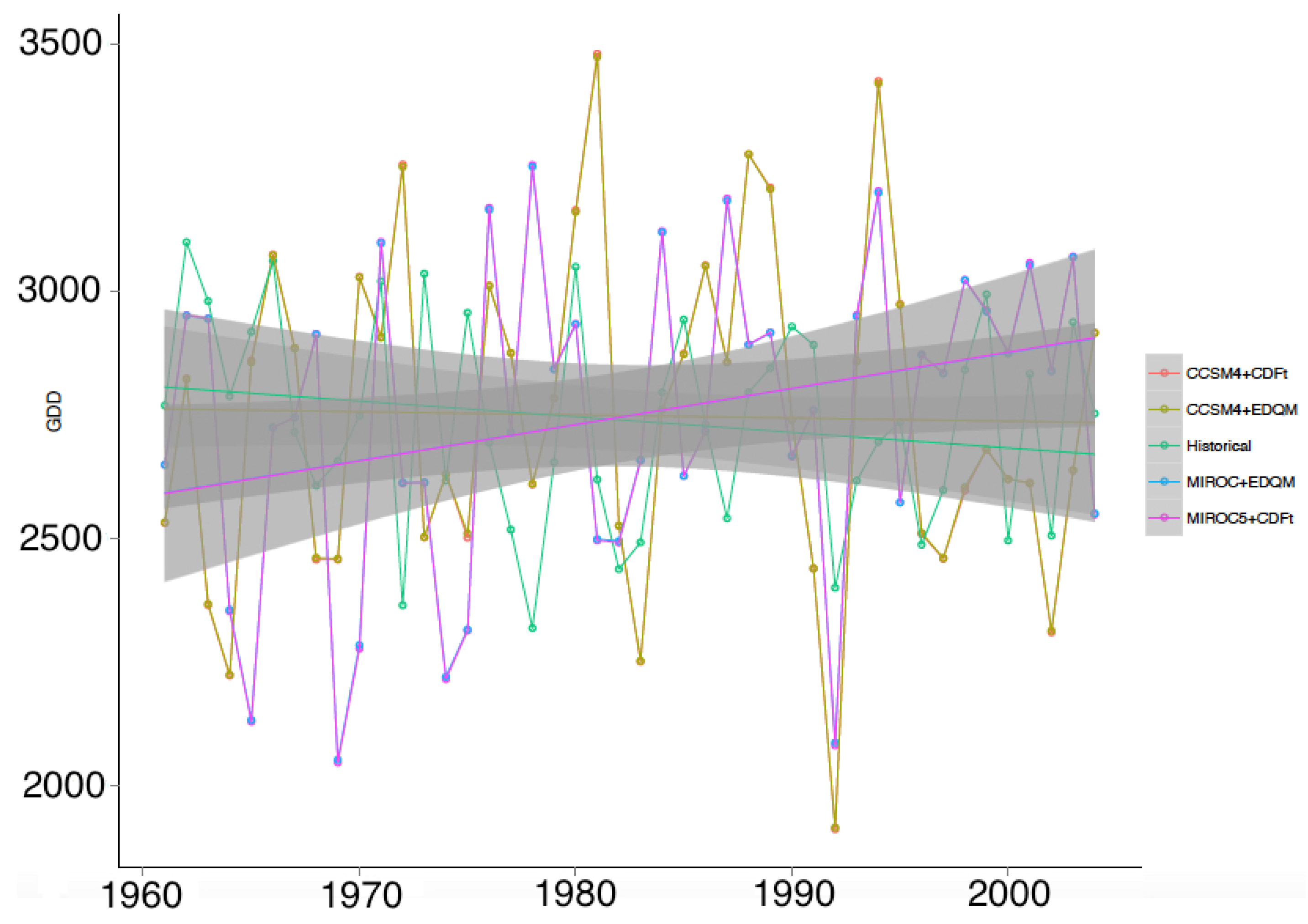
3.1. Historical Period

The historical period consists of the growing seasons from 1961 to 2004. Figure 3 shows the area mean historical GDD and the area mean timing until reaching 1825 GDD over the study region, calculated from the historical 1/10th degree observation-based dataset. The figure highlights the multi-annual variability over the historical period, with variations in the GDD between 3100 °C and 2320 °C (Figure 3a); with their respective timings varying by ~40 days (Figure 3b). The historical time-series shown in Figure 3 have multiannual mean values of 2738 °C and 220 days, respectively.

In particular, when analyzing the downscaled output from the CCSM4 and MIROC5 GCMs over the historical period, the number of GDDs varies spatially from 2400 °C to 3600 °C. As seen in Figure 4, there are no substantial spatial differences between the GDD obtained from the CDFt and the EDQM methods, although the CCSM4 model output produced higher values of GDD over the southeastern region of the domain. Overall, there are marginal differences between the spatial patterns of CCSCM- and the MIROC5-derived projections over the historical period.

Bias Correction

The historical GDD simulations from the statistically downscaled datasets were compared to those from the observation-based dataset. The analysis showed that, on average, the simulations reached 1825 GDD 20 to 21 days earlier than in the historical (observed) data. These differences in the timing were caused by GDD mean biases between the downscaled output and the observations (440–445 degrees). Therefore, we bias-corrected the historical and future GDD simulations accordingly, and adjusted the winter wheat’s (projected) mean time before harvest. Figure 5 shows the annual variability between the GDD from the observed historical dataset and the downscaled historical time series. The results show that the downscaled output from the MIROC5 has a slight positive trend, while their counterparts from the CCSM4 and the observations show a small negative trend in the GDD, with higher accumulations at the end of the historical period. The figure also highlights that, in general, the results from the different GCM/downscaling combinations have higher variability than the one from the observations.

Hereafter, when we mention the results derived from the statistically downscaled datasets, we refer to the bias-corrected versions.

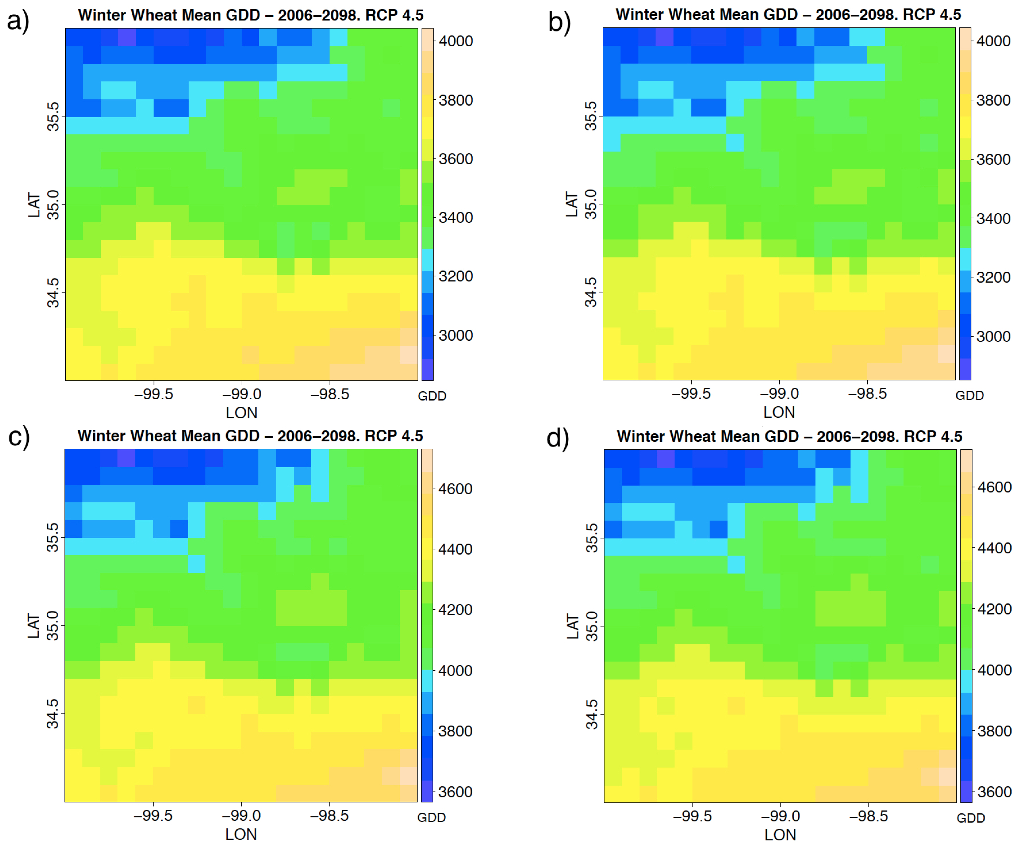
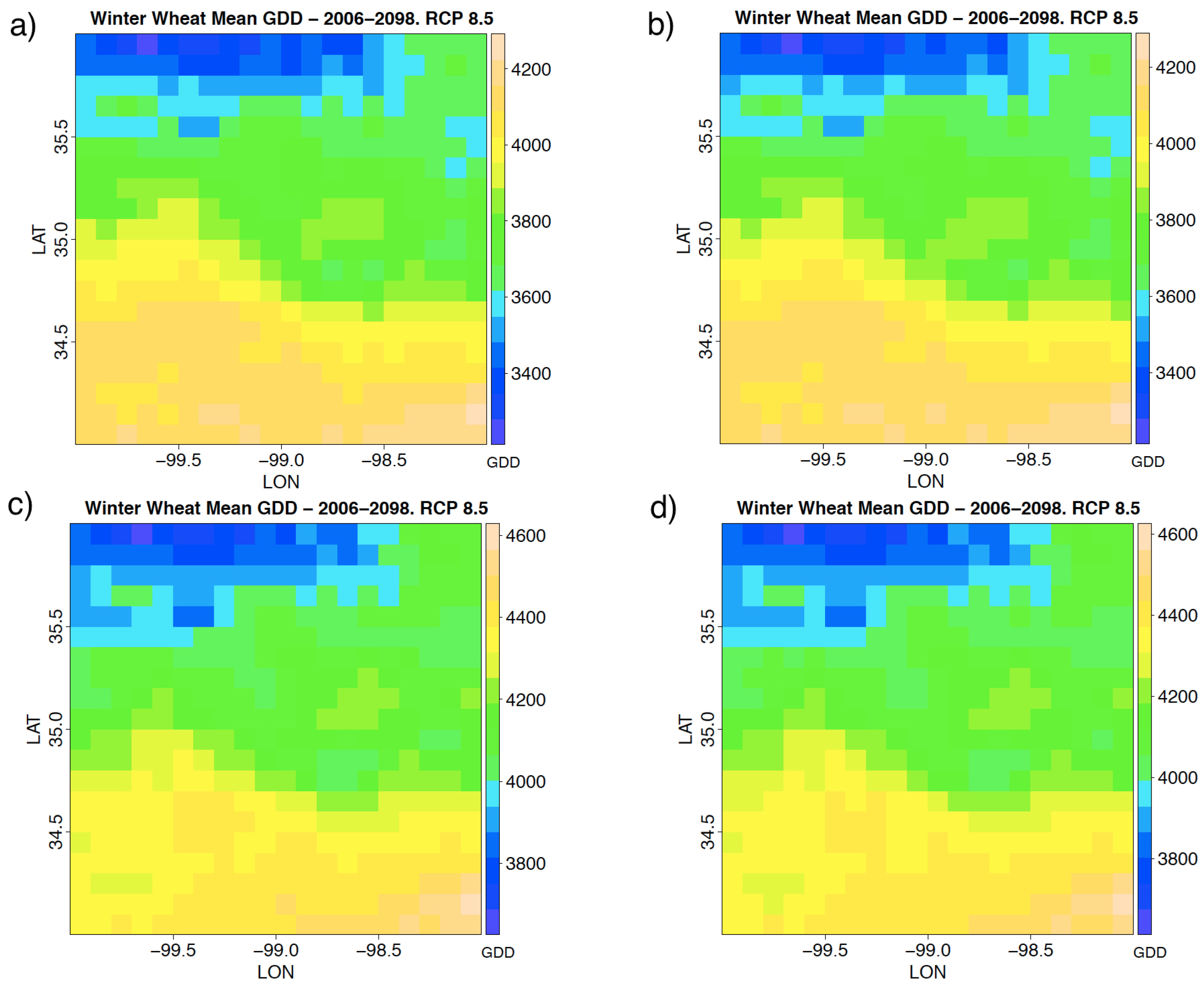
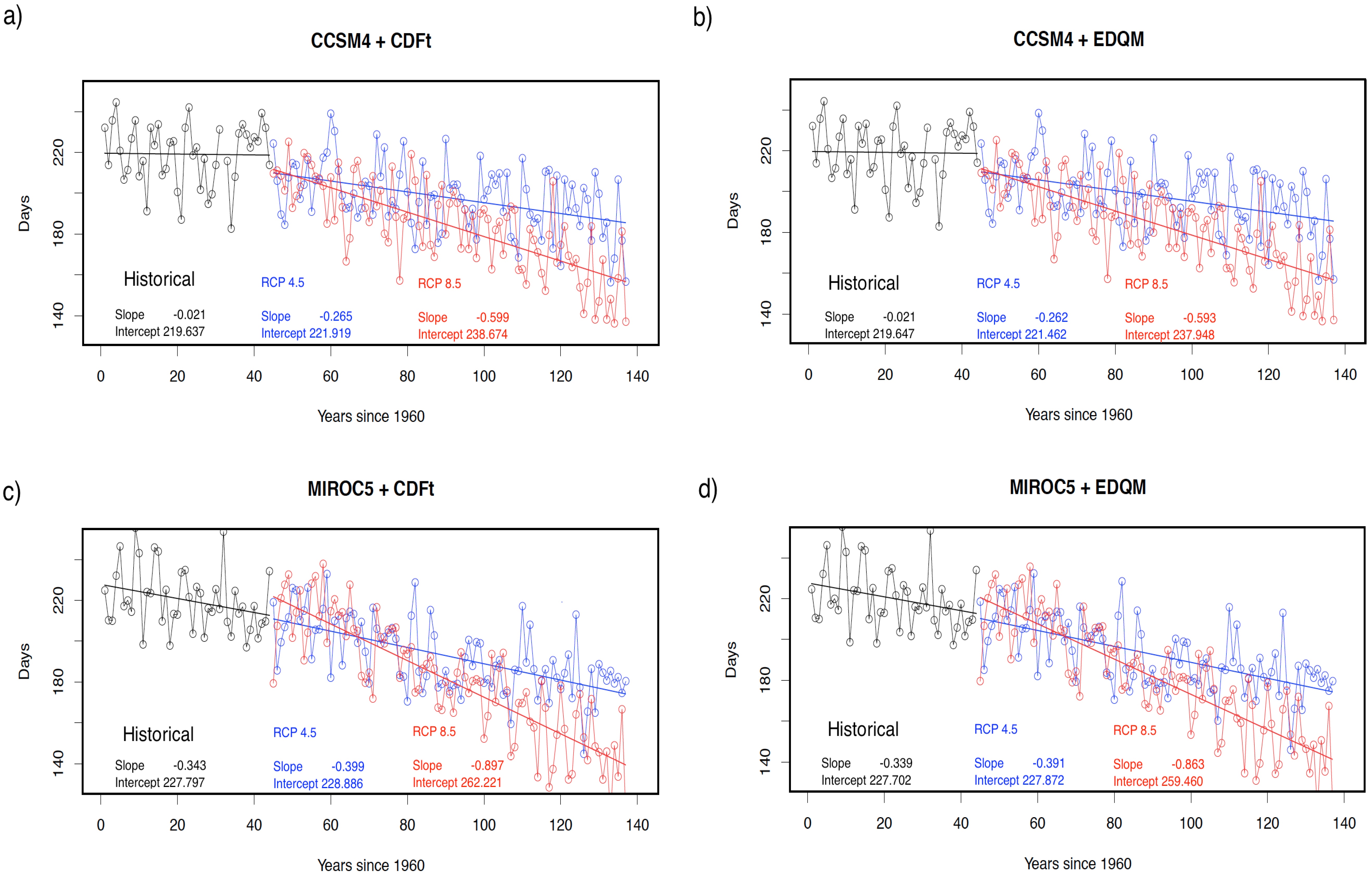
3.2. Future Period (2006–2098)

RCP 4.5 and RCP 8.5

The future period analysis covered the growing seasons from 2006 to 2098. These results were derived from the downscaled projections from the CCSM4 and MIROC5 models using the EDQM and CDFt methods. The future projections were obtained assuming the RCP 8.5 and the RCP 4.5 pathways.

For RCP 4.5 (Figure 6), the spatial patterns from the four GCM/downscaling combinations were similar; however, when looking closely at the CCSM4 downscaled output, the range of GDD results varied between 3000 °C and 4000 °C, in contrast to the 3600 °C–4600 °C range obtained from the MIROC5. As expected, the RCP4.5 future projections exceeded the 2400 °C–3600 °C historical range.

The results from RCP 8.5 are shown in Figure 7. In general, when looking at the multiannual means, the minimum number of GDDs changed more than 400 °C in comparison with the RCP 4.5 results. Similarly, for those projections derived from the MIROC5 GCM, the maximum number of GDDs over the region changed to 4600 °C. Overall, both the CDFt and the EDQM methods showed similar spatial patterns when downscaling the same GCM. Therefore, we speculate that for this study, the highest source of uncertainty comes from the GCMs and not from the downscaling methods used.

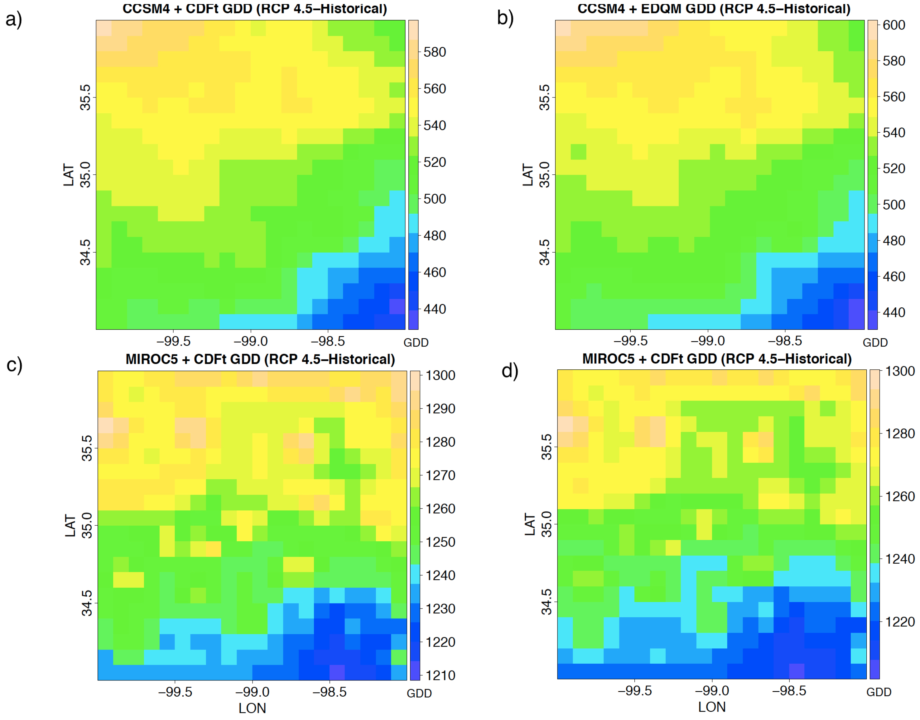
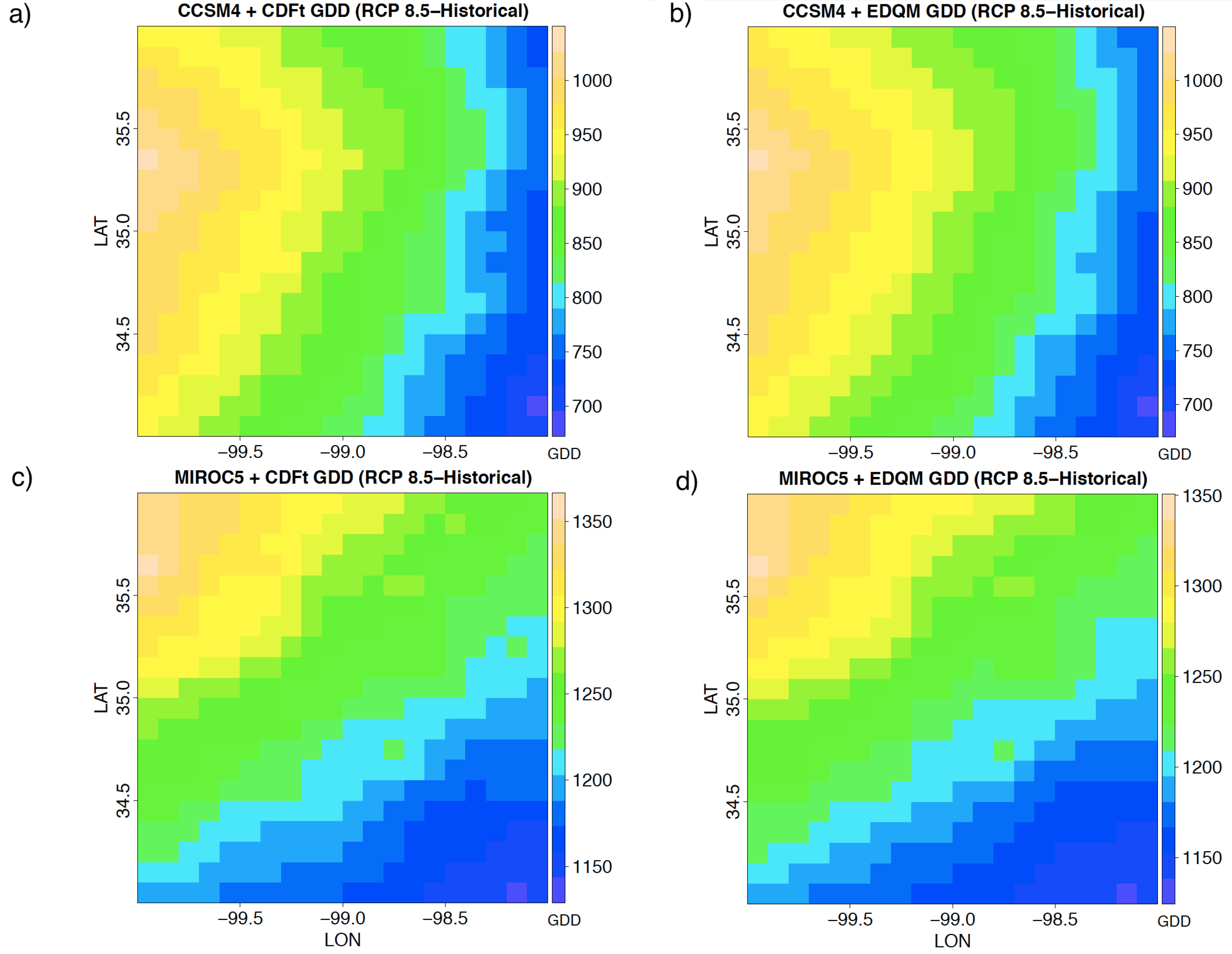
3.3. Mean Differences Between Past and Future Periods

Figure 8 and Figure 9 show the mean GDD differences between the historical and future periods for the RCP 4.5 and the RCP 8.5 future projections. The differences were found by subtracting the mean values from the historical period from those of the future period.

In Figure 8 (RCP 4.5 downscaled projections minus historical counterparts), when analyzing the differences from the CCSM4-derived projections (Figure 8a,b), the future mean GDD could increase between 440 °C and 600 °C from the historical average, with the larger differences projected in the northwestern part of the domain. On the other hand, when looking at the GDD differences from the MIROC5 model, the results vary between 1210 °C and 1300 °C, and had a more heterogeneous spatial pattern than the CCSM4-based projections. Nevertheless, these projections showed more noticeable changes over the northern part of the study region than over the southern region.

On the other hand, the differences between the RCP 8.5-derived projections and their historical counterparts (Figure 9) show dissimilar change patterns for the CCSM4-based and the MIROC5-based projections. The CCSM4 projections show East-West gradients, with the western part of the domain projecting mean changes of up to 1000 °C, in comparison to the ~700 °C projected over the eastern boundary of the domain. In contrast, the MIROC5 projections show a diagonal gradient with larger changes projected over the northwestern region and fewer changes over the southeastern region; however, the magnitude of the changes from the MIROC5-derived projections (Figure 9c,d) are substantially higher than the ones from the CCSM4 model (Figure 9a,b).

These results show that the CCSM4 model, regardless of the downscaling method, projected a higher number of GDDs when compared to the downscaled projections from the MIROC5—as demonstrated in Figure 6 and Figure 7. In general, the CCSM4 GCM projects more warming over the region, which will affect the future GDD.

To end, we analyzed the changes in the timing (number of days required to accumulate 1825 °C, Figure 10). The results show that all the future projections (CCSM4 + CDFt, CCSM4 + EDQM, MIROC5 + CDFt and MIROC5 + EDQM) for both RCPs (4.5 and 8.5) have a significant trend projecting an overall decrease on the number of days required to reach 1825 °C. In particular, Figure 10 shows in black the downscaled historical time series for the CCSM4 and MIROC5 models. The CCSM4-derived results show no trend while the MIROC5-derived historical time series show a slight decreasing trend.

Further, as expected, all the projections from the RCP 8.5 (red) have a steeper negative slope than the ones from the RCP 4.5 (blue). In general, the RCP 4.5 (and to a minor extent RCP 8.5) shows very mild changes versus the historical period during the first three to four decades of this century, and arguably, the annual variability during this period is projected to be similar to the historical one. In contrast, the timing of the GDD only becomes markedly different from the historical values during the last part of the 21st century. However, both RCP 4.5 and 8.5 show a decrease in the number of days needed to accumulate 1825 GDD.

4. Conclusions and Discussion

Here we used two GCM, two quantile mapping methods and two RCPs (4.5 and 8.5) to analyze the projected changes in GDD and growing season timing of winter wheat over the 21st century. We focused our analysis on a highly productive region in Oklahoma. Our analysis complements previous studies on winter wheat that used only one downscaling method (either dynamical or statistical) to obtain the local scale information. In this study, we corrected the biases between the simulated GDD from the downscaled output and the GDD from the historical data.

In particular, when looking at the downscaled outputs from a single GCM (MIROC5 or CCSM4) we found out that the results from the CDFt and the EDQM methods were similar. However, when the results of the two GCMs were compared, we observed a wider range of GDDs and discrepancies in the spatial patterns of GDD. Overall, for this particular location, the projected changes in GDDs of winter wheat mainly depend on the GCM used and not as much on the downscaling method employed. Moreover, the varying future outputs from the GCMs caused significant spatial and temporal variations over the region, even after bias-correcting the output. This result partially supplements [25], as their results using different GCMs and one downscaling method showed that the winter wheat yields were location dependent and varied with the GCM used. For their assessment, they used two GCMs and a weather generator to obtain local scale information. Overall, given the uncertainty associated with the different GCM outputs, we suggest that practitioners cautiously apply these projections to crop models, especially if they are interested in analyzing the second half of the 21st century.

On the other hand, when using the downscaled output from the CCSM4 and RCP 4.5, Southwest Oklahoma is expected to accumulate more GDDs than in the historical period within the designated domain. The results show that at the end of the 2098 growing season, the increase in GDDs is expected to be between 440 °C and 1300 °C, for RCP 4.5, and between 700 °C and 1350 °C for RCP 8.5. The marginal difference between the upper ranges derived from the RCPs partially agree with [8], where they mentioned that very little contrast in winter wheat’s yield was based on the future projections (using emission scenarios, not RCPs, as in our case).

Overall, the increase in GDDs might decrease the number of days required to reach crop maturity, and all the GCM/downscaling combinations showed a decreasing trend in these timings during the 21st century. This could potentially mean that the winter wheat will grow quicker and will have to be harvested earlier than normal [37]. Our result is also consistent with the findings of [24] where the projected higher temperatures shortened the growing season and increased the plants’ heat stress, and with [8], where yield projections of maize, rice and winter wheat derived from dynamically downscaled outputs showed a decrease in the growing season over the southeastern United States.

As the GDD varied over the region forming a gradient from the southeastern to the northwestern region of the domain, the winter wheat on the northwestern side of the domain will accumulate more heat units than the rest of the domain. On the other hand, when using the downscaled projections from the MIROC5 GCM, the mean change over the 21st century is projected to be more heterogeneous across the study region, with the higher accumulations occurring in the northern part of the domain.

When looking at the future projections based on RCP 8.5 in terms of multiannual means, the minimum number of GDDs changed more than 400 °C in comparison with the RCP 4.5 results. Similarly, the maximum number of GDDs over the region changed to 4600 °C (MIROC5 + downscaled). Overall, both the CDFt and the EDQM methods showed similar patterns. Therefore, we consider that for this study, the highest source of uncertainty comes from the GCMs and not the downscaling methods used.

Our results show that the GCM uncertainty is more impactful than the downscaling uncertainty when calculating GDDs and associated timing over the region. Here, we used two GCMs that performed adequately over the region; however, the differences between the GDDs calculated from both climate models were considerable. Overall, as mentioned by [39] a more adequate quantification of uncertainty might lead to greater confidence in our assessments of the impacts of climate change on crop yield.

Something that is of utmost importance is to estimate potential yield loss or gain due to the changing climate in the South-central region. One line of thought states that the dominant warming trend should benefit farmers growing winter wheat, as a higher GDD accumulation could allow farmers to grow better yielding varieties; however, [40] states that, “…longer growing seasons in these regions do not necessarily translate into an increase in yield, and with further climate change, extremely high temperatures may limit crop growth in more areas in the future”. Similarly, [24] argued that an increase in temperature will cause the crops to mature sooner, which should lower the expected yields (assuming all other factors being constant over time). Moreover, others argued that as the climate continues to become drier and hotter, crop growth will reach a threshold and then decline. Here, we noticed that the future projections from both GCMs show similar inter-annual variability as the historical period for the next 3–4 decades, and only in the second half of the century does the GDD and its timing show values outside of the ones from the late 20th century. We speculate that this can give the farmers more time to adapt, as the projections from the near future are similar to values that they have already experienced.

As some farmers use their land for dual-purpose (for grazing pasture and then to produce crops), they rely on earlier sowing. Unfortunately for the farmers, water is a very limited resource. In Southwest Oklahoma, many farmers do not have access to center pivot irrigation, so rain-fed crops dominate the area. If even less water is available in the future, it would “increase the demand for irrigation or reduce productivity in regions where not enough water is allocated or no infrastructure is available for irrigation”, and would thus increase the “water wars” occurring between municipalities and the agriculture sector [39].

In the last few years, many Oklahoman farmers have had their crops severely damaged by late freezes. Wheat that is planted earlier is at a disadvantage because of its maturity stage when the freeze arrives. Researchers and farmers would soon have to collaborate on establishing a breeding program that, overtime, increases wheat's cold hardiness. If not, farmers will have to switch to another crop that is much heartier and drought-resistant. The farming landscape known today could be vastly different in the future.

We acknowledge that our experimental setup is limited by the stationarity assumption inherent to all the statistical downscaling methods, and that our conclusions are limited to four combinations of GCMs and quantile mapping techniques (i.e., MIROC5 + CDFt, MIROC5 + EDQM, CCSM4 + CDFt and CCSM + EDQM); further studies might look into expanding the number of GCMs and/or downscaling methods used, and into incorporating decision tools that will help the farmers to operate under deep uncertainty [40]. Similarly, we acknowledge that other factors related to the growth of winter wheat such as precipitation, soil type, wheat variety, infestations and many more were not taken into account (See [41] for an example of empirical methods using precipitation and fertilizer data to predict maize yield). The study of these factors might provide further understanding about climate change impacts on winter wheat. Moreover, we speculate that the addition of these parameters might improve the spatio-temporal representation of the GDDs over the region, as the effects on the temperature changes on the simulation of photosynthesis, respiration, evapotranspiration and yield are non-linear [24].

References

1. USDA. Briefing on the Status of Rural America. Available online: http://www.usda.gov/documents/Briefing_on_the_Status_of_Rural_America_Low_Res_Cover_update_map.pdf (accessed on 15 July 2015).
2. EPA. Ag 101. Available online: https://www.epa.gov/sites/production/files/2015-07/documents/ag_101_agriculture_us_epa_0.pdf (accessed on 10 July 2015).
3. McKlusky, P.J. Enciclopedia of the Great Plains. University of Nebraska Lincoln. 2011. Available online: http://plainshumanities.unl.edu/encyclopedia/doc/egp.ag.075 (accessed on 2 July 2015).
4. IPCC. Climate Change 2014: Impacts, Adaptation, and Vulnerability. Part A: Global and Sectoral Aspects; Contribution of Working Group II to the Fifth Assessment Report of the Intergovernmental Panel on Climate Change; Cambridge University Press: Cambridge, UK, 2014; p. 1132. [Google Scholar]
5. IPCC. Climate Change 2014: Impacts, Adaptation, and Vulnerability. Part B: Regional Aspects; Contribution of Working Group II to the Fifth Assessment Report of the Intergovernmental Panel on Climate Change; Cambridge University Press: Cambridge, UK, 2014; p. 688. [Google Scholar]
6. Parthasarathi, T.; Velu, G.; Jeyakumar, P. Impact of crop heat units on growth and developmental physiology of future crop production: A review. Res. Rev. J. Crop Sci. Technol. 2013, 2, 1–11. [Google Scholar]
7. Miller, P.; Lanier, W.; Brandt, S. Using growing degree days to predict plant stages. Montana State University Extension Service Montguide. 2000. Available online: http://store.msuextension.org/publications/AgandNaturalResources/MT200103AG.pdf (accessed on 1 September 2016).
8. Tsvetsinskaya, E.A.; Mearns, L.O.; Mavromatis, T.; Gao, W.; McDaniel, L.; Downton, M.W. The Effect of Spatial Scale of Climatic Change Scenarios on Simulated Maize, Winter Wheat, and Rice Production in the Southeastern United States. Climatic Change 2003, 60, 37–72. [Google Scholar] [CrossRef]
9. Gaitan, C.F.; Hsieh, W.W.; Cannon, A.J.; Gachon, P. Evaluation of Linear and Non-Linear Downscaling Methods in Terms of Daily Variability and Climate Indices: Surface Temperature in Southern Ontario and Quebec, Canada. Atmosphere-Ocean 2013, 52, 211–221. [Google Scholar] [CrossRef]
10. Li, H.; Sheffield, J.; Wood, E.F. Bias correction of monthly precipitation and temperature fields from intergovernmental panel on climate change ar4 models using equidistant quantile mapping. J. Geophys. Res. 2010, 115, D10101. [Google Scholar] [CrossRef]
11. Gaitán, C.F. Effects of variance adjustment techniques and time-invariant transfer functions on heat wave duration indices and other metrics derived from downscaled time-series. Study case: Montreal, Canada. Nat. Hazards 2016, 81, 1661. [Google Scholar] [CrossRef]
12. Branzuela, N.E.; Faderogao, F.J.F.; Pulhin, J.M. Downscaled Projected Climate Scenario of Talomo-Lipadas Watershed, Davao City, Philippines. J. Earth Sci. Clim. Chang. 2015, 6, 268. [Google Scholar]
13. Milly, P.C.D.; Betancourt, J.; Falkenmark, M.; Hirsch, R.M.; Kundzewicz, Z.W.; Lettenmaier, D.; Stouffer, R.J. Stationarity is Dead: Whiter Water Management. Science 2008, 319, 573–574. [Google Scholar] [CrossRef] [PubMed]
14. Gaitan, C.F.; Cannon, A.J. Validation of historical and future statistically downscaled pseudo-observed surface wind speeds in terms of annual climate indices and daily variability. Renew. Energy 2013, 51, 489–496. [Google Scholar] [CrossRef]
15. Gaitan, C.F.; Hsieh, W.W.; Cannon, A.J. Comparison of statistically downscaled precipitation in terms of future climate indices and daily variability for southern Ontario and Quebec, Canada. Clim. Dyn. 2014, 43, 3201–3217. [Google Scholar] [CrossRef]
16. Anwar, M.R.; Liu, D.L.; Macadam, I.; Kelly, G. Adapting agriculture to climate change: A review. Theor. Appl. Climatol. 2013, 113, 225–245. [Google Scholar] [CrossRef]
17. Criveanu, R.C.; Sperdea, N.M. Organic agriculture, climate change, and food security. Econ. Manag. Financ. Mark. 2014, 9, 118–123. [Google Scholar]
18. Howden, S.M.; Soussana, J.-F.; Tubiello, F.N.; Chhetri, N.; Dunlop, M.; Meinke, H. Adapting Agriculture to Climate Change. Proc. Natl. Acad. Sci. USA 2007, 104, 19691–19696. [Google Scholar] [CrossRef] [PubMed]
19. Kang, M.S.; Banga, S.S. Global Agriculture and Climate Change. J. Crop Improv. 2013, 27, 667–692. [Google Scholar] [CrossRef]
20. Rickards, L.; Howden, S.M. Transformational adaptation: Agriculture and climate change. Crop Pasture Sci. 2012, 63, 240–250. [Google Scholar] [CrossRef]
21. Riehl, S. Climate and agriculture in the ancient Near East: A synthesis of the archaeobotanical and stable carbon isotope evidence. Veg. Hist. Archaeobot. 2008, 17, S43–S51. [Google Scholar] [CrossRef]
22. Scialabba, N.E.-H.; Müller-Lindenlauf, M. Organic agriculture and climate change. Renew. Agric. Food Syst. 2010, 25, 158–169. [Google Scholar] [CrossRef]
23. Stål, H.I.; Bonnedahl, K.J. Provision of Climate Advice as a Mechanism for Environmental Governance in Swedish Agriculture: Climate Advice and Environmental Governance in Swedish Agriculture. Environ. Policy Gov. 2015, 25, 356–371. [Google Scholar] [CrossRef]
24. Brown, R.A.; Rosenberg, N.J. Climate change impacts on the potential productivity of corn and winter wheat in their primary United States growing regions. Climatic Change 1999, 41, 73–107. [Google Scholar] [CrossRef]
25. Weiss, A.; Hays, C.J.; Won, J. Assessing winter wheat responses to climate change scenarios: A simulation study in the U.S. great plains. Climatic Change 2003, 58, 119–147. [Google Scholar] [CrossRef]
26. Kellogg, W. Impacts of Climate Change on Flows in the Red River Basin; USGS: Norman, OK, USA, 2014.
27. Gaitan, C.F. Statistically Downscaled Time Series for the Red River Basin; Gaitan, C.F., Ed.; University of Oklahoma Libraries: Princeton, NJ, USA, 2016. [Google Scholar] [CrossRef]
28. Gaitan, C.F. 1/10th of a Degree Observation-Based Dataset; Gaitan, C.F., Ed.; University of Oklahoma Libraries: Princeton, NJ, USA, 2016. [Google Scholar] [CrossRef]
29. Gaitan, C.F. Downscaled Climate Variables from MIROC5 GCM; Gaitan, C.F., Ed.; University of Oklahoma Libraries: Princeton, NJ, USA, 2016. [Google Scholar] [CrossRef]
30. Gaitan, C.F. Downscaled Climate Variables from CCSM4 GCM; Gaitan, C.F., Ed.; University of Oklahoma Libraries: Princeton, NJ, USA, 2016. [Google Scholar] [CrossRef]
31. Gent, P.R.; Danabasoglu, G.; Donner, L.J.; Holland, M.M.; Hunke, E.C.; Jayne, S.R.; Lawrence, D.M.; Neale, R.B.; Rasch, P.J.; Vertenstein, M.; et al. The Community Climate System Model Version 4. J. Clim. 2011, 24, 4973–4991. [Google Scholar] [CrossRef]
32. Watanabe, M.; Suzuki, T.; O’ishi, R.; Komuro, Y.; Watanabe, S.; Emori, S.; Takemura, T.; Chikira, M.; Ogura, T.; Sekiguchi, M.; et al. Improved Climate Simulation by MIROC5: Mean States, Variability, and Climate Sensitivity. J. Clim. 2010, 23, 6312–6335. [Google Scholar] [CrossRef]
33. Sheffield, J.; Barrett, A.P.; Colle, B.; Fernando, D.N.; Fu, R.; Geil, K.L.; Hu, Q.; Kinter, J.; Kumar, S.; Langenbrunner, B.; et al. North American Climate in CMIP5 Experiments. Part I: Evaluation of Historical Simulations of Continental and Regional Climatology. J. Clim. 2013, 26, 9209–9245. [Google Scholar] [CrossRef]
34. Livneh, B.; Rosenberg, E.A.; Lin, C.; Nijssen, B.; Mishra, V.; Andreadis, K.M.; Maurer, E.P.; Lettenmaier, D.P. A Long-Term Hydrologically Based Dataset of Land Surface Fluxes and States for the Conterminous United States: Update and Extensions. J. Clim. 2013, 26, 9384–9392. [Google Scholar] [CrossRef]
35. Michelangeli, P.-A.; Vrac, M.; Loukos, H. Probabilistic downscaling approaches: Application to wind cumulative distribution functions. Geophys. Res. Lett. 2009, 36, L11708. [Google Scholar] [CrossRef]
36. Gaitan, C.F. Downscaled Climate Variables from MPI-ESM-LR GCM; Gaitan, C.F., Ed.; University of Oklahoma Libraries: Princeton, NJ, USA, 2016. [Google Scholar]
37. Steduto, P.; Hsiao, T.C.; Fereres, E.; Raes, D. FAO Irrigation and Drainage Paper 66, Crop Yield Response. Available online: http://www.fao.org/docrep/016/i2800e/i2800e.pdf (accessed on 7 September 2016).
38. FAO. Crop Water Information: Wheat. Available online: http://www.fao.org/nr/water/cropinfo_wheat.html (accessed on 3 July 2015).
39. Chalinor, A.J.; Wheeler, T.R.; Osborne, T.M.; Slingo, J.M. Assessing the Vulnerability of Food Systems to Climate Change Thresholds Using an Integrated Crop-Climate Model. Available online: http://stabilisation.metoffice.com/53_Dr_Andrew_Challinor.pdf (accessed on 7 September 2016).
40. Mueller, B.; Hauser, M.; Iles, C.; Rimi, R.H.; Zwiers, F.W.; Wan, H. Lengthening of the growing season in wheat and maize producing regions. Weather Clim. Extremes 2015, 9, 47–56. [Google Scholar] [CrossRef]
41. Matsumura, K.; Gaitan, C.F.; Sugimoto, K.; Cannon, A.J.; Hsieh, W.W. Maize yield forecasting by linear regression and artificial neural networks in Jilin, China. J. Agric. Sci. 2014, 153, 399–410. [Google Scholar] [CrossRef]
Figure 1. Gridded spatial mask of the Red River Basin (United States of America). Spatial resolution 1/10th degree. Black square indicates the study area.
Agriculture 06 00047 g001
Figure 2. Performance assessment of the selected Global Climate Models (GCM) based on Central North America biases. Climate sensitivity based on [32] (left), and GCM mean temperature bias over North America during winter (DJF) and summer seasons (JJA) based on [33] (right).
Agriculture 06 00047 g002
Figure 3. (a) Mean number of Growing Degree Days (GDD) over the region, and (b) mean number of days until reaching the target GDD (1825 °C) during the historical period.
Agriculture 06 00047 g003
Figure 4. Mean Growing Degree Days derived from the Global Climate Model (GCM) historical runs (1961–2004) and four GCM/downscaling model combinations: (a) outputs for the CCSM4 GCM and Cumulative Density Function transfer (CDFt) downscaling method. (b) outputs for the CCSM4 GCM and the Equidistant Quantile Mapping (EDQM) downscaling method. (c) outputs for the MIROC5 GCM and CDFt downscaling method. (d) outputs for the MIROC5 GCM and EDQM downscaling method.
Agriculture 06 00047 g004
Figure 5. Annual variability between the GDD from the observed historical dataset and the downscaled historical time series.
Agriculture 06 00047 g005
Figure 6. Mean GDD derived from the RCP 4.5 future projections (2006–2098) and four GCM/downscaling model combinations: (a) Top left—outputs for the CCSM4 GCM and CDFt downscaling method, (b) Bottom left-outputs for the CCSM4 GCM and EDQM downscaling method, (c) Top right—outputs for the MIROC5 GCM and CDFt downscaling method and, (d) Bottom right shows the outputs for the MIROC5 GCM and EDQM downscaling method.
Agriculture 06 00047 g006
Figure 7. Mean GDD derived from the RCP 8.5 future projections (2006–2098) and four GCM/downscaling model combinations: (a) Top left—outputs for the CCSM4 GCM and CDFt downscaling method. (b) Bottom left—outputs for the CCSM4 GCM and EDQM downscaling method. (c) Top right—outputs for the MIROC5 GCM and CDFt downscaling method. (d) Bottom right shows the outputs for the MIROC5 GCM and EDQM downscaling method.
Agriculture 06 00047 g007
Figure 8. Mean differences between the outputs of the historical period (1961–2004) and the future period (2006–2098)—RCP 4.5 simulation. (a) outputs for the CCSM4 GCM and CDFt downscaling method. (b) outputs for the CCSM4 GCM and EDQM downscaling method. (c) outputs for the MIROC5 GCM and CDFt downscaling method. (d) the outputs for the MIROC5 GCM and EDQM downscaling method.
Agriculture 06 00047 g008
Figure 9. Mean differences between the outputs of the historical period (1961–2004) and the future period (2006–2098)—RCP 4.5 simulation. (a) outputs for the CCSM4 GCM and CDFt downscaling method. (b) outputs for the CCSM4 GCM and EDQM downscaling method. (c) outputs for the MIROC5 GCM and CDFt downscaling method. (d) the outputs for the MIROC5 GCM and EDQM downscaling method.
Agriculture 06 00047 g009
Figure 10. Number of days needed to reach 1825 GDD over the study period (1960–2099).
Agriculture 06 00047 g010