
Asymmetric Price Transmission: A Case of Wheat in India


1
ICAR-Indian Agricultural Statistics Research Institute, New Delhi 110012, India
2
Upper Assam Advisory Center, Tea Research Association, Dikom 786101, India
*
Author to whom correspondence should be addressed.
Agriculture 2022, 12(3), 410; https://doi.org/10.3390/agriculture12030410
Submission received: 30 December 2021
/
Revised: 17 January 2022
/
Accepted: 4 February 2022
/
Published: 15 March 2022
(This article belongs to the Topic New Trends in Agri-Food Sector: Environmental, Economic and Social Perspectives)
Abstract
:In the present paper, horizontal and vertical integration was carried out on the wholesale and retail prices of wheat in the major markets of India. On confirming cointegration between the wholesale and retail prices of wheat in all needs, the vector error correction model (VECM) was applied to find the speed of adjustment in the corresponding price channel. The results revealed that price signals are transmitted across regions, indicating that price changes in one market are consistently related to price changes in markets and can influence the prices in other markets. In addition to studying cointegration, threshold autoregressive (TAR) and Momentum TAR (MTAR) models were applied to test for asymmetric cointegration. Hasen and Seo’s test was used to test for the presence of threshold cointegration. It revealed a significant presence of asymmetric and nonlinear cointegration in many markets. Accordingly, a threshold VECM (TVECM) model with two regimes was applied. The results indicate that the retail price significantly responds to the deviations from the long-run equilibrium compared to the wholesale price.
1. Introduction
India ranks second in the world after China regarding wheat production and consumption. India’s share in global wheat production was recorded at 12.76 percent in 2016–2017. India has been self-sufficient in wheat production. India’s share in global exports was around 0.40 percent in 2015–2016 (Directorate General of Commercial Intelligence and Statistics (DGCI&S). As per the 2016–2017 data collected from the Directorate of Economics and Statistics, Ministry of Agriculture and Farmers′ Welfare, Government of India, it was revealed that the highest share of wheat comes from Uttar Pradesh (30% of total production), followed by Madhya Pradesh (18%), Punjab (17%), Haryana (12%), and Rajasthan (9%), which together share about 86% of the total national wheat production while Gujarat contributes the remaining 14% including Maharashtra, Uttarakhand, West Bengal, and other states of the country. The leading states in terms of area under wheat are Uttar Pradesh, Madhya Pradesh, Punjab, Haryana, and Rajasthan, accounting for more than 80 percent of wheat area in the country.
Market integration is a concept used to determine how markets of goods and services related to one another experience similar patterns in terms of an increase or decrease in the cost of commodities. The term can also be related to circumstances in which the costs of relatable goods and services sold in a defined geographical location also start to move in a similar pattern. Therefore, market integration is the phenomenon by which price interdependence takes place. Agricultural product markets established under market regulation programs play a vital role in providing marketplaces for farmers to sell their products. These markets also offer facilities and environments to the traders, processors, and other market functionaries for the smooth conduct of their trading activities. Agricultural commodities are characterized by seasonality, variability, perishability, etc. Poor market integration is relatively uncompetitive. Scrappy and small farms with a low volume of marketable surplus makes the market difficult to perform.
The marketed surplus from production has also been rising, and it is estimated that about 60–70 percent of the production now comes to market. As a result, India’s marketing system and efficiency are of significant concern and interest. Poor marketing efficiency can have severe consequences for both producers and consumers and affects government policy and the economy. Significant concerns have been raised regarding working the market mechanisms and market-related policies for wheat, a staple food crop. The market price of grain necessarily influences the demand for wheat. The demand-side market of wheat products needs to be explored to understand the impact on the production and growth of the crop. It is necessary to look at the price movement of wheat in different markets due to mismatch between demand–supply and large-scale imports.
Market integration is generally composed of two types: horizontal market integration and vertical market integration. Horizontal market integration indicates that the price of a commodity in one market responds to a change in the price of the same product in other markets. Vertical market integration represents the integration of the cost of the same product at different levels of the value chain (farm price, wholesale price, and retail price).
Usually, market reforms are required in order to achieve efficient agricultural markets and production systems. The producers and consumers in the marketing chain can realize the potential gains from the common market when the markets are integrated. In this regard, the prices of wheat play a vital role. When the markets are integrated, the price signals are transmitted from one call to another and influence other market prices. The wholesale market prices (producer′s level) and retail market (consumer′s level) prices are essential components of the marketing process. Studying the market integration of wheat has become necessary due to the interdependence of wholesale and retail markets. Price transmission can be of two types: symmetric and asymmetric. In contrast to symmetric price transmission, asymmetric price transmission (APT) is said to exist when the adjustment of prices is not homogeneous concerning external or internal characteristics of the system. Significant causes of asymmetric price transmission are non-competitive markets and adjustment costs [1]. Perez-Mesa et al. [2] investigated retail price rigidity in perishable food products and reported that price asymmetry was not avoided despite the relaxation of bargaining power.
2. Background
In the literature, several empirical studies have been carried out using cointegration techniques that concern the market integration of agricultural commodities in India and other countries. Asche et al. [3] carried out vertical and horizontal price linkages for salmon and found a high degree of price transmission in both supply chains and integrated markets in salmon. The price convergence across various regions in India was investigated by [4] and their results indicated a significant presence of cross-sectional dependence in prices in India. Jha et al. [5] stated that local food scarcity would persist if agricultural markets are not integrated. Balaguer and Ripollés [6] studied integration among transport fuel retail markets in Spain, and the future trading of soybean in India using a cointegration approach was studied in [7]. The non-linear error correction model was applied to assess price linkages and patterns of transmission among producer and consumer markets for apple in Slovenia [8]. Paul et al. [9] studied the volatility and associations between domestic and export prices of onion in India. The market integration of coffee prices in primary markets of India was studied by [10]. Gricar and Bojnec [11] investigated the causalities between Slovenian tourism and macroeconomic aggregate, and they reported that input costs were significant drivers for the rise in Slovenian hospitality industry prices. Ricci et al. [12] studied the effects of price instability in agriculture on vertical price transmission in Italy. The market integration using monthly price data for 21 agricultural goods and 60 markets in India was carried out by [13]. The authors reported no robust evidence that price integration has increased in recent years. Gricar et al. [14] applied the vector error correction model (VECM) and found that hospitality prices in Montenegro were domestic driven and in Slovenia Eurozone driven. However, little work has been carried out on empirically evaluating wheat market integration in India. Empirical evaluation of intra-state and inter-state spatial integration of wheat markets in India was carried out in [15], where strong evidence favoring the spatial integration of regional wheat markets was reported. Gandhi and Zhou [16] indicated that in India, wheat production is concentrated, and growth is driven predominantly by yield increases, and to some extent, by a shift in the area from other crops. Mukim et al. [17] established that the wheat markets are integrated across states of India in the long-run, but not in the short-run. All of these studies concentrated on the spatial (horizontal) market integration of wheat; there is hardly any work related to India’s vertical integration of wheat prices.
However, unlike the above studies, the prices of many commodities including wheat are characterized by asymmetric adjustment [18,19]. Meyer and Von Cramon-Taubadel [1] studied the different types and causes of asymmetric price transmission and described the econometric techniques used to quantify it. Enders and Granger [20] investigated the asymmetric movements toward long-run equilibrium. In this situation, it is essential to use the threshold cointegration approach, which allows for the asymmetric adjustment introduced by [21]. The authors reported that if price adjustment is asymmetric, then the standard cointegration tests and extensions are not correctly specified. In the literature, estimation methods of threshold cointegration have been extensively studied [22,23]. The structure of interest rates by the threshold cointegration model was studied in [24]. The price–transmission dynamics in the Iranian egg market was studied by [25]. Asymmetric panel vector error correction model (VECM) was applied to study the price transmission mechanism along the European food supply chain [26]. Price asymmetry in Bangladesh rice markets was studied by [27]. The nonlinear autoregressive distributed lag (NARDL) model was utilized to study the rice trade in Southeast Asia [28]. Threshold cointegration and asymmetric error-correction approaches were applied to investigate the nexus between India’s current and capital accounts [29]. However, the application of threshold cointegration in agriculture is scarce. The present study deals with market integration in wheat prices both horizontally and vertically. Moreover, there is no study of asymmetric cointegration in wheat prices in Indian markets. Therefore, the present study attempts to examine the movement of wheat prices in different markets across the states of India and the transmission of price signals and information across these markets. For this purpose, threshold autoregressive (TAR) and momentum-TAR (MTAR) approaches have been applied [30]. A good description of asymmetric integration may be found in [31].
3. Data and Methodology
The study was undertaken covering seventeen major markets: Delhi, Jammu, Amritsar, Ludhiana, Lucknow, Dehradun, Raipur, Ahmedabad, Bhopal, Mumbai, Jaipur Patna, Bhubaneswar, Bengaluru, Thiruvananthapuram, Chennai, and Hyderabad, along with the all India maximum, minimum, and modal price of wheat. Daily data on retail and wholesale prices of wheat of the above markets from January 2010 to May 2018 were collected from the Department of Consumer Affairs, Government of India [32]. The Jarque–Bera test statistics were used to check the normality of the series. Wholesale price is the price at which when the retailers buy products in large volumes. Retail prices are what retailers set as the final selling price for consumers. The daily data were converted into weekly data. The missing observations were imputed by using the mean value (i.e., if the 3rd week of January 2015 is missing, it is replaced by the mean of the 3rd week price of January of preceding years). The econometric methods used in the present investigation are described below in brief. These techniques allow one to quantify the degree of interconnectedness between the markets. In order to check for the presence of unit root, the tests, namely the augmented Dickey–Fuller (ADF) test [33], Phillips–Perron unit root test [34], and KPSS test [35] were used.
3.1. Johansen’s Approach to Cointegration
The multivariate cointegration approach [36] examines the cointegration among price series. Let yt be n × 1 set of I(1) variables (if the series is integrated to order d, it is denoted as I(d)). Usually, any linear combination will be I(1) for a ≠ 0. However, if there exists an n × 1 vector αi such that is , , then it is said that the components in yt are cointegrated of order one, denoted CI(1) with the cointegrating vector as αi. It can be noted that if αi is a cointegrating vector, then so is the kαi for any k ≠ 0, since .
For the total n series, there can be maximum r different cointegrating vectors, where 0 ≤ r = k − 1 < n.
3.2. Error Correction Models (ECM)
The ECM can be written as per Equation (1) in vector and matrix notation.
where α = [α1, α2]′, β′ = [1, −β1], and .
Equation (1) can be reformulated into a vector error correction model (VECM):
where , I = 1,…, k − 1, and . The estimates and , respectively explain the short and long-run adjustments to changes in yt.
Here, , where α represents the rate of adjustments and β is a matrix of long-run coefficients. The optimum lag length is selected based on the minimum value of the information criterion (e.g., Akaike information criterion (AIC) and Baysian information criterion (BIC)).
3.3. Asymmetric Cointegration
The standard cointegration tests and their extensions are mis-specified if the adjustment is asymmetric [21]. Furthermore, to capture asymmetry in a cointegrating relationship, the authors extended the threshold autoregressive (TAR) and momentum threshold autoregressive (M-TAR) models of [20] to a multivariate context. The aspects of ‘deep movements’ can be captured by the TAR model while ‘steep movements′ in a price is captured by M-TAR ([20]). Hassanzoy et al. [19] reported that the M-TAR model is superior to that of TAR and the Engle and Granger tests. In the present investigation, in order to take care of the large changes in the price series, the M-TAR model was applied. The consistent M-TAR model is defined by Equations (3)–(5). Here, the speed of adjustment toward equilibrium depends on the direction of change in , that is, Δ. Therefore, the speed of adjustment is ρ1, if deviations from the long-run equilibrium are positive, and ρ2otherwise.
where is a threshold value; ρ1 and ρ2 are adjustment coefficients; indicates the coefficient(s) of lagged changes; and ωt is the identically independently distrusted (i.i.d.) stochastic term. The necessary and sufficient conditions for stationarity of are ρ1 < 0, ρ2 < 0, and (1 + ρ1) (1 + ρ2) < 1 for any values of [18,19]. Tong [37] showed that the least square estimates of ρ1 and ρ2 had an asymptotic multivariate normal distribution under the condition that is stationary. The M-TAR model was applied in this paper to examine the long-run relationship among the pairs of wholesale and retail prices of wheat assuming asymmetric adjustment. For threshold cointegration with M-TAR adjustment, the five-step procedure reported in [19] was followed. First, a long-run relationship between the pairs of markets was estimated as follows:
where y1,t and y2,t are the logarithm of wholesale and retail prices of wheat at time t; is a constant term; is th elasticity of price transmission; and εt is the error term that may be serially correlated. In the second step, following [38], consistent estimates of threshold values for M-TAR models were obtained. Equations (3) and (4) were estimated for each of the possible threshold values. Finally, the threshold () was estimated by minimizing the sum of squared residuals from the fitted model. In the third step, the null hypothesis of no cointegration, that is, ρ1 = ρ2 = 0, was tested for each of the M-TAR models. Fourth, the null hypothesis of no asymmetric adjustment, that is, ρ1 = ρ2, was tested for each of the M-TAR models using the standard F-test under the condition that the null hypothesis of no cointegration is rejected. In the last step, the Ljung–Box Q-statistic was applied to test for the white noise process of the estimated residuals from the M-TAR models. Once the presence of cointegration was established among the markets, the dynamics of price transmission among them were analyzed using asymmetric vector error correction models (AVECMs) with threshold (M-TAR) adjustment. On application of the TAR model, it revealed that asymmetric cointegration was present in the wholesale and retail prices of wheat in the markets, namely Ahmedabad, Bengaluru, Bhubaneswar, Hyderabad, Patna and the all India minimum price. On the other hand, using the MTAR model, it was seen that asymmetric cointegration was present in most markets.
4. Results and Discussion
Summary statistics of the price data of different markets were computed and are reported in Table 1. It can be seen that both the wholesale and retail prices were more or less consistent in the markets as depicted by the coefficient of variation (CV) value. In the market integration study, the first step is to check for evidence of the non-stationarity of data. Test for stationarity was performed by using the ADF test, PP test, and the KPSS test. The results of all three tests, as reported in Table 2, revealed that all variables were non-stationary. In order to achieve stationarity, the series were differenced to the first order and all series became stationary after the first differentiation. As all the series were found to be integrated of the same order, the dataset was suitable for cointegration.
Cointegration in Price Series
Johansen′s cointegration test has been applied to investigate cointegration among different markets with respect to wholesale and retail prices. For horizontal integration, 11 markets were selected based on the production and consumption of wheat in different states of India. The 11 selected markets were: Ahmedabad, Amritsar, Bhopal, Dehradun, Delhi, Jaipur, Jammu, Lucknow, Ludhiana, Mumbai, and Patna. It revealed that markets were perfectly cointegrated with respect to wholesale as well as retail price. Both the maximum eigenvalue statistic and trace statistics were used to test the cointegration and the results are reported in Table 3. In retail price, according to the trace statistics, the no. of cointegrating equations was six, whereas the eigen value statistics indicate that the no. of cointegrating equations was two. Similarly, for wholesale price, no. of cointegrating equations was found to be four and three, respectively, based on the trace and eigenvalue statistics. In addition to the horizontal cointegration, the vertical cointegration between the wholesale and retail prices of wheat in an individual market was also investigated. The results of Johansen’s cointegration test are presented in Table 4 using the trace and eigen statistics. It was observed that the wholesale and retail prices were integrated in all markets.
Before investigating the presence of asymmetric cointegration, the presence of nonlinearity was tested using the BDS test [39]. The results of the BDS test is reported in Table 5. The results indicate that all of the series were nonlinear in nature. After assuring cointegration among the wholesale and retail prices of wheat, test of the presence of asymmetric cointegration was investigated by means of the MTAR model, as described in Section 3.3. The results of the asymmetric cointegration tests are presented in Table 6. In Table 6, Phi determines whether retail and wholesale prices are cointegrated or not and APT (asymmetric price transmission) checks whether price transmission between individual markets of retail and wholesale price is of a symmetric or asymmetric nature. The MTAR model revealed that Delhi, Ahmedabad, Bhopal, Chennai, Hyderabad, Jaipur, Jammu, Lucknow, Ludhiana, Maximum, Minimum, and Modal series had the property of APT.
The acceptance of cointegration between two series implies that there exists a long-run relationship between them and means that an error correction model (ECM) is applicable, which combines the long-run relationship with the short-run dynamics of the model. Accordingly, the vector error correction model (VECM) was applied in order to find the speed of adjustment and long-run coefficient among wholesale and retail prices of wheat in individual markets. For fitting of the VECM model, first, an unrestricted VAR model was fitted and optimum lag was determined based on the Akaike information criterion (AIC) and Bayesian information criteria (BIC). The results of VECM is reported in Table S1 in the Supplementary Materials. In the markets of Delhi, Bhopal, Mumbai, Jaipur, Patna, and Bhubaneswar, the optimum number of lags for wholesale and retail prices was one lag; whereas in all the other markets, the optimum number of lags for wholesale and retail prices was found to be two. It was noted that most of the values of the error correction term (ECT) that are significant were found to be negative. The value of ECT signifies the speed of adjustment at which the market approaches equilibrium once it deviates. The speed of adjustment (per week) was found to be highest in Jaipur (18.8%), followed by Bhopal (17.4%), Lucknow (13%), and Hyderabad (13%) in retail price. However, in the case of wholesale price, the Jammu market had the highest speed of adjustment (13.2%) toward equilibrium.
For instance, the error correction model (ECM) for the Ahmedabad market can be written as
where and respectively denotes the retail and wholesale price at time t. and denotes the error correction term respectively for the retail and wholesale price equation.
Subsequent to applying VECM, the Sup-LM test [22] was applied to test the null hypothesis of linear cointegration against the two-regime threshold cointegration. The result of the Sup-LM is reported in Table 7. It can be seen from Table 7 that in the markets of Delhi, Ahmedabad, Bhopal, Hyderabad, Jammu, Mumbai, Patna, Thiruvananthapuram, all India minimum and modal price, the mechanism of the price transmission was not linear, but was rather of a threshold type.
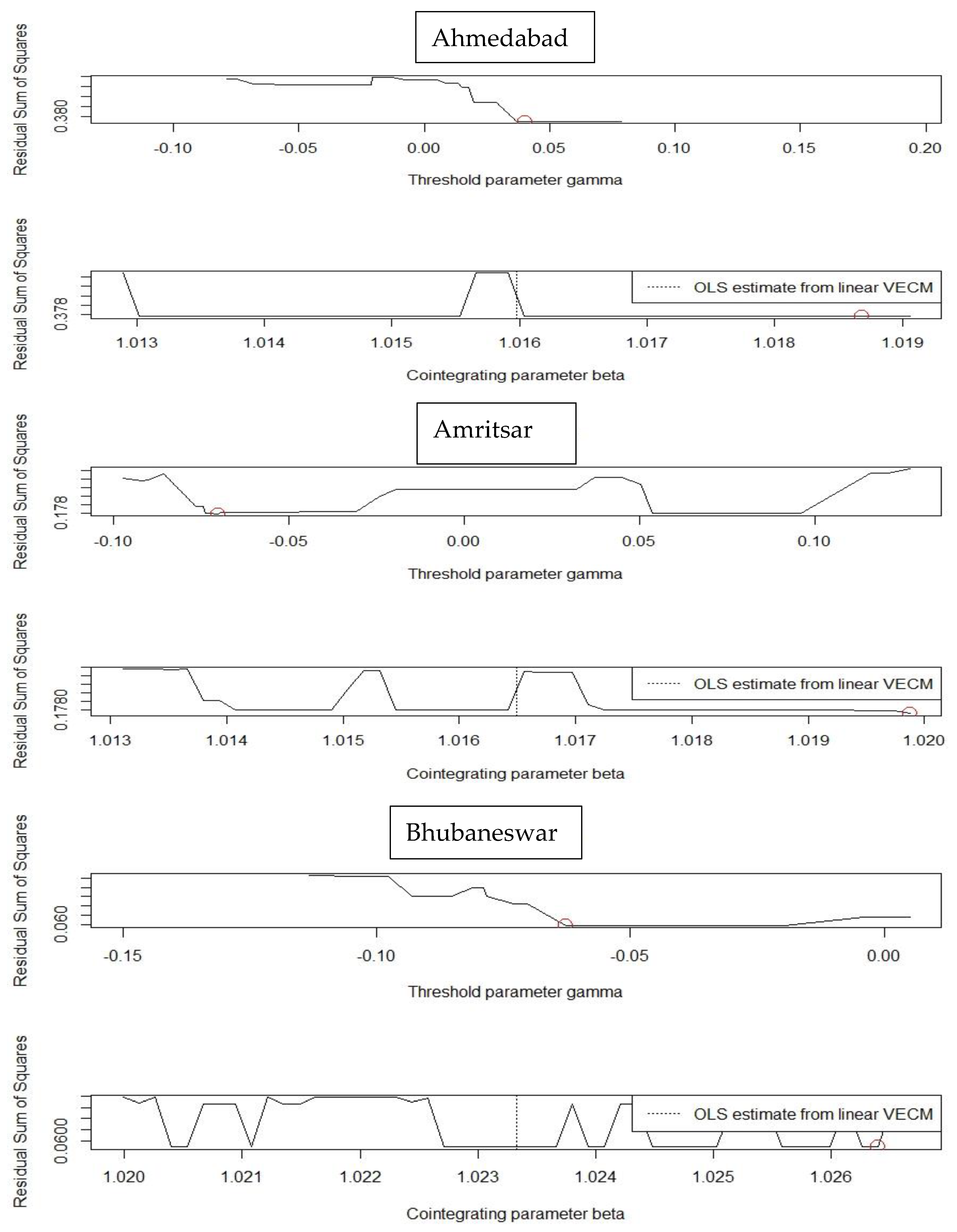
Accordingly, to accommodate the asymmetricity and nonlinearity in price transmission as clearly shown in Table 5 and Table 6, threshold VECM was fitted with two regimes and the results are reported in Table S2 in the Supplementary Materials. The percentage of data points fell in the first regime and the second regime is mentioned in the second to last column in Table S2 and the threshold value as found in the individual market to divide the data in two regimes is mentioned in the last column of Table S2. The approach followed to find the optimum lag in the TVECM model was the same as that of the VECM model. The optimum value as obtained through the grid search is depicted in Figure 1. To save space, the optimum value of the threshold parameter and the cointegration parameter obtained through grid search only for the selected markets, namely, Ahmadebad, Amritsar, and Bhubaneswar are depicted in Figure 1. In the present investigation, in almost all markets, there was a significant difference in the percent of observations falling into the first and second regime except for Bhubaneswar and Chennai. In Bhubaneswar, 46.30% of observations fell in the first regime while 53.70% of observations fell in the second regime. Similarly, in Chennai, 45.50% of observations fell in the first regime and 54.50% of observations fell in the second regime. According to Hansen and Seo [22], it can be called a “typical” regime, where more than half of the observations belong to this regime, and the regime that includes a lower percent of the observations is known as an “extreme” regime. Therefore, the short-run dynamic effects of the retail and wholesale prices show significant differences between typical and extreme regimes.
5. Discussion
The existence of both horizontal and vertical cointegration among the studied series implies that there exists a long-run relationship and an error correction model (ECM) that combines the long-run relationship with the short-run dynamics of the model. The results indicate that most of the error correction terms (ECTs) were statistically significant, implying that the system, once in disequilibrium, tries to come back to the equilibrium state (e.g., in Bhopal, the retail price once it deviates from equilibrium, approaches toward equilibrium at the rate of 9.6% per week (ECT = −0.096)). Furthermore, the existence of asymmetric cointegration was observed in more than 50% of the studied markets. Application of the two-regime TVECM demonstrated that the coefficient of ECT was significant in retail for both the regimes in Delhi; wholesale for both the regime and retail in typical regime for Jammu; retail and wholesale in the extreme regime for Amritsar; retail in both regimes, but wholesale in the extreme regime for Ludhiana; retail in the extreme regime in Lucknow; retail in both regimes for Dehradun; wholesale in a typical regime and retail in an extreme regime for Ahmedabad; retail in both regimes for Bhopal; retail in the extreme regime and wholesale in a typical regime for Mumbai; wholesale in a typical regime and retail in an extreme regime for Jaipur; retail and wholesale both in the extreme regime for Patna; retail and wholesale in both regimes; retail in the extreme regime for Bengaluru; retail in the typical regime for Thiruvananthapuram; wholesale in the second regime for Chennai; and retail in both regimes and wholesale in a typical regime for Hyderabad. This implies that retailers respond significantly to the deviations from the long-run equilibrium.
6. Conclusions
In the present study, presence of cointegration was tested by using Johansen’s approach. It was revealed that wholesale and retail prices of wheat in all markets were cointegrated both horizontally as well as vertically. For horizontal integration, it was revealed that markets were spatially cointegrated with respect to wholesale as well as retail prices. This indicates that information on change in the wholesale/retail price in one market is transmitted to the other spatially integrated markets. In addition to the horizontal cointegration, the vertical cointegration between the wholesale and retail prices of wheat in individual markets was also investigated. It was observed that a change in wholesale price in a market is reflected in the change in retail price in the same market.
Asymmetricity in price transmission was investigated by means of TAR and M-TAR models. Application of the MTAR model revealed that most of the markets under consideration were asymmetric in terms of price transmission from wholesale to retail markets. Moreover, our findings pointed out that there are nonlinearities in the studied price adjustment process. To ensure asymmetricity as well as nonlinearity in cointegration and price transmission between the wholesale and retail prices of wheat, the TVECM model was applied. It can be seen that the price signals are transmitted across both the horizontal and vertical chain. However, the direction and intensity of price changes may be affected by the dynamic linkages between the demand and supply. The results from the study will help improve the precision of the information to predict the price movements used by marketing operators to formulate appropriate strategies. As the forecast of the wholesale (retail) price of a commodity will not only depend on changes in its own lag prices, but also on the changes in lags of the retail (wholesale) prices of that commodity. Similarly, for prediction of the wholesale price of a commodity in a market, the lagged wholesale price of that market along with lagged prices of other integrated markets need to be considered.
The study will help policy makers design suitable marketing strategies in bringing efficiency in agricultural markets. It is noted that price changes are temporary and would converge to an equilibrium within a given time span. Consideration of proper domestic supply management and international trade, along with strong market surveillance, will minimize the gap between the wholesale and retail prices of agricultural commodities. The present study has some limitations as this did not highlight the factors that affect the price of the commodity in a cointegraton study. This may be explored in future research. Furthermore, in studying vertical cointegration, the farm harvest price of the commodity may be included.
Supplementary Materials
The following supporting information can be downloaded at: https://www.mdpi.com/article/10.3390/agriculture12030410/s1, Table S1: Results of VECM model; Table S2: Results of TVECM model; Table S3: Granger Causality test results.
Author Contributions
Conceptualization, R.K.P. and T.K.; Formal analysis, R.K.P.; Investigation, R.K.P.; Methodology, R.K.P. and T.K.; Writing—review and editing, R.K.P. and T.K. All authors have read and agreed to the published version of the manuscript.
Funding
This research received no external funding.
Informed Consent Statement
Not applicable.
Data Availability Statement
The data were collected from the Department of Consumer Affairs, Government of India.
Acknowledgments
The authors are grateful to the two anonymous reviewers for their extensive comments that helped in improving the quality of this manuscript.
Conflicts of Interest
The authors declare that there are no conflict of interest in publishing this manuscript.
References
- Meyer, J.; Von Cramon-Taubadel, S. Asymmetric price transmission: A survey. J. Agric. Econ. 2004, 55, 581–611. [Google Scholar] [CrossRef] [Green Version]
- Perez-Mesa, J.; Galdeano-Gómez, E.; Aznar-Sánchez; José, A. Retail price rigidity in perishable food products: A case study. Span. J. Agric. Res. 2010, 8, 895–907. [Google Scholar] [CrossRef] [Green Version]
- Asche, F.; Jaffry, S.; Hartmann, J. Price transmission and market integration: Vertical and horizontal price linkages for salmon. Appl. Econ. 2007, 39, 2535–2545. [Google Scholar] [CrossRef]
- Das, S.; Bhattacharya, K. Price convergence across regions in India. Empir. Econ. 2008, 34, 299–313. [Google Scholar] [CrossRef] [Green Version]
- Jha, R.; Bhanu Murthy, K.V.; Sharma, A. Markets Market Integration in Wholesale Rice in India. In The Indian Economy Sixty Years after Independence; Jha, R., Ed.; Palgrave Macmillan: London, UK, 2008. [Google Scholar]
- Balaguer, J.; Ripollés, J. Are the transport fuel retail markets regionally integrated in Spain? Evidence from price transmission. Econ. Model. 2014, 42, 323–332. [Google Scholar] [CrossRef]
- Bhardwaj, S.P.; Paul, R.K.; Kumar, A. Future trading in soybean—An econometric analysis. J. Indian Soc. Agric. Stat. 2015, 69, 11–17. [Google Scholar]
- Hassouneh, I.; Serra, T.; Bojnec, Š. Nonlinearities in the Slovenian apple price transmission. Br. Food J. 2015, 117, 461–478. [Google Scholar] [CrossRef]
- Paul, R.K.; Saxena, R.; Chaurasia, S.; Zeeshan, M.; Rana, S. Examining export volatility, structural breaks in price volatility and linkages between domestic & export prices of onion in India. Agric. Econ. Res. Rev. 2015, 28, 101–116. [Google Scholar]
- Paul, R.K.; Sinha, K. Spatial market integration among major coffee markets in India. J. Indian Soc. Agric. Stat. 2015, 69, 281–287. [Google Scholar]
- Sergej, G.; Bojnec, S. Tourism price causalities: Case of an Adriatic country. Int. J. Tour. Res. 2018, 20, 82–87. [Google Scholar]
- Ricci, E.C.; Peri, M.; Baldi, L. The Effects of Agricultural Price Instability on Vertical Price Transmission: A Study of the Wheat Chain in Italy. Agriculture 2019, 9, 36. [Google Scholar] [CrossRef] [Green Version]
- Andrle, M.; Blagrave, P. Agricultural Market Integration in India. IMF Work. Pap. 2020, 20. [Google Scholar] [CrossRef]
- Gričar, S.; Bojnec, S.; Karadžić, V.; Backović, T. Tourism price normalities in two Adriatic east coast “euro” countries. Econ. Res. Ekon. Istraživanja 2021. [Google Scholar] [CrossRef]
- Ghosh, M. Spatial Integration of Wheat Markets in India: Evidence from Cointegration Tests. Oxf. Dev. Stud. 2003, 31, 159–171. [Google Scholar] [CrossRef]
- Gandhi, V.P.; Zhou, Z.Y. India’s Wheat Economy: Will Demand Be a Constraint or Supply? Econ. Political Wkly. 2004, 39, 4737–4746. [Google Scholar]
- Mukim, M.; Singh, K.; Kanakaraj, A. Market Integration, Transaction Costs and the Indian Wheat Market: A Systematic Study. Econ. Political Wkly. 2009, 44, 149–155. [Google Scholar]
- Hassanzoy, N.; Ito, S.; Isoda, H.; Amekawa, Y. A comparison of asymmetric price transmission from global to domestic markets between high and low quality grains: A case of Afghan rice markets. Econ. Bull. 2016, 36, 537–552. [Google Scholar]
- Hassanzoy, N.; Ito, S.; Isoda, H.; Amekawa, Y. Cointegration and spatial price transmission among wheat and wheat-flour markets in Afghanistan. Appl. Econ. 2017, 49, 2939–2955. [Google Scholar] [CrossRef]
- Enders, W.; Granger, C.W.J. Unit root tests and asymmetric adjustment with an example using the term structure of interest rates. J. Bus. Econ. Stat. 1998, 16, 304–311. [Google Scholar]
- Enders, W.; Siklos, P.L. Cointegration and threshold adjustment. J. Bus. Econ. Stat. 2016, 19, 166–176. [Google Scholar] [CrossRef] [Green Version]
- Hansen, B.E.; Seo, B. Testing for two regime threshold cointegration in vector error-correction models. J. Econom. 2002, 110, 293–318. [Google Scholar] [CrossRef] [Green Version]
- Seo, M.H. Estimation of nonlinear error correction models. Econ. Theory 2011, 27, 201–234. [Google Scholar]
- Wang, M.; Chan, N.H.; Yau, C.Y. Nonlinear error correction model and multiple-threshold cointegration. Stat. Sin. 2016, 26, 1479–1498. [Google Scholar] [CrossRef]
- Aghabeygi, M.; Antonioli, F.; Arfini, F. Assessing symmetric price transmission by using threshold cointegration in Iranian egg market. Br. Food J. 2021, 123, 2278–2288. [Google Scholar] [CrossRef]
- Rezitis, A.N.; Rokopanos, A. Asymmetric Price Transmission along the European Food Supply Chain and the CAP Health Check: A Panel Vector Error Correction Approach. J. Agric. Food Ind. Organ. 2019, 17, 20180002. [Google Scholar] [CrossRef]
- Deb, L.; Lee, Y.; Lee, S.H. Market Integration and Price Transmission in the Vertical Supply Chain of Rice: An Evidence from Bangladesh. Agriculture 2020, 10, 271. [Google Scholar] [CrossRef]
- Wiseman, T.; Luckstead, J.; Durand-Morat, A. Asymmetric Exchange Rate Pass-Through in Southeast Asian Rice Trade. J. Agric. Appl. Econ. 2021, 53, 341–374. [Google Scholar] [CrossRef]
- Mallick, L.; Behera, S.R.; Murthy, R.R. Dynamics of capital account and current account in India: Evidence from threshold cointegration with asymmetric error correction. Appl. Econ. Lett. 2021, 1–6. [Google Scholar] [CrossRef]
- Tiwari, A.K.; Mutascu, M. The revenues-spending nexus in Romania: A TAR and MTAR approach. Econ. Res. Ekon. Istraživanja 2015, 29, 735–745. [Google Scholar] [CrossRef] [Green Version]
- Bagnai, A.; Opsina, C.A.M. Asymmetries, Outliers, and Structural Stability in the US Gasoline Market. Energy Econ. 2018, 69, 250–260. [Google Scholar] [CrossRef]
- DCA. Department of Consumer Affairs, Ministry of Consumer Affairs, Food and Public Distribution, Government of India. 2020. Available online: https://fcainfoweb.nic.in/reports/report_menu_web.aspx (accessed on 12 October 2020).
- Dickey, D.A.; Fuller, W.A. Distribution of the estimators for autoregressive time series with a unit root. J. Am. Stat. Assoc. 1979, 74, 427–431. [Google Scholar]
- Phillips, P.C.B.; Perron, P. Testing fora unit root in time series regression. Biometrika 1988, 75, 335–346. [Google Scholar] [CrossRef]
- Kwiatkowski, D.; Phillips, P.C.B.; Schmidt, P.; Shin, Y. Testing the null hypothesis of stationarity against the alternative of a unit root. J. Econom. 1992, 54, 159–178. [Google Scholar] [CrossRef]
- Johansen, S. A statistical analysis of cointegration vectors. J. Econ. Dyn. Control. 1988, 12, 231–254. [Google Scholar] [CrossRef]
- Tong, H. Threshold models in time series analysis—30 years on. Stat. Its Interface 2011, 4, 107–118. [Google Scholar] [CrossRef] [Green Version]
- Chan, K.S. Consistency and limiting distribution of the least squares estimator of a threshold autoregressive model. Ann. Stat. 1993, 21, 520–533. [Google Scholar] [CrossRef]
- Brock, W.; Dechert, D.; Scheinkman, J.; LeBaron, B. A test for independence based on the correlation dimension. Econom. Rev. 1996, 15, 197–235. [Google Scholar] [CrossRef]
- Granger, C.W.J. Some recent developments in the concept of causality. J. Econom. 1988, 39, 199–211. [Google Scholar] [CrossRef]
Figure 1.
Grid search to find the optimum value of the threshold parameter and cointegration parameter in TVECM.
Figure 1.
Grid search to find the optimum value of the threshold parameter and cointegration parameter in TVECM.

Table 1.
Descriptive statistics for the wholesale and retail prices (INR per quintal) of the individual markets.
Table 1.
Descriptive statistics for the wholesale and retail prices (INR per quintal) of the individual markets.
| Markets | Wholesale Price | Retail Price | ||||||||||
|---|---|---|---|---|---|---|---|---|---|---|---|---|
| Mean | Median | Max | Min | SD | CV(%) | Mean | Median | Max | Min | SD | CV(%) | |
| Ahmedabad | 1647.75 | 1650.00 | 2000.00 | 1100.00 | 302.89 | 18.38 | 1851.49 | 1900.00 | 2300.00 | 1200 | 318.11 | 17.18 |
| Amritsar | 1491.28 | 1500.00 | 1900.00 | 1050.00 | 229.44 | 15.39 | 1688.93 | 1800.00 | 2200.00 | 1100 | 297.61 | 17.62 |
| Bengaluru | 2320.10 | 2500.00 | 2800.00 | 1671.43 | 418.44 | 18.04 | 2582.08 | 2700.00 | 3400.00 | 1800 | 530.42 | 20.54 |
| Bhopal | 1457.20 | 1500.00 | 1700.00 | 1050.00 | 170.97 | 11.73 | 1638.73 | 1700.00 | 2000.00 | 1100 | 234.91 | 14.33 |
| Bhubaneswar | 1512.65 | 1580.00 | 1580.00 | 1210.00 | 107.36 | 7.10 | 1803.18 | 1800.00 | 2014.29 | 1400 | 222.5 | 12.34 |
| Chennai | 2298.40 | 2342.86 | 2814.29 | 1800.00 | 204.42 | 8.89 | 2794.45 | 3000.00 | 3500.00 | 2000 | 439.36 | 15.72 |
| Dehradun | 1511.74 | 1512.86 | 1880.00 | 1120.00 | 218.85 | 14.48 | 1709.16 | 1600.00 | 2200.00 | 1200 | 310.24 | 18.15 |
| Delhi | 1590.37 | 1671.43 | 2227.86 | 1138.57 | 244.90 | 15.40 | 1800.62 | 1900.00 | 2414.29 | 1300 | 234.88 | 13.04 |
| Hyderabad | 2359.37 | 2400.00 | 2700.00 | 1490.71 | 356.55 | 15.11 | 2581.75 | 2700.00 | 2900.00 | 1700 | 353.88 | 13.71 |
| Jaipur | 1570.16 | 1600.00 | 2250.00 | 1150.00 | 233.97 | 14.90 | 1709.90 | 1700.00 | 2600.00 | 1300 | 256.55 | 15.00 |
| Jammu | 1562.63 | 1617.14 | 2560.00 | 1000.00 | 253.82 | 16.24 | 1698.18 | 1700.00 | 2200.00 | 1100 | 259.59 | 15.29 |
| Lucknow | 1445.64 | 1450.00 | 1900.00 | 1035.71 | 215.18 | 14.88 | 1576.59 | 1600.00 | 2000.00 | 1100 | 213.26 | 13.53 |
| Ludhiana | 1489.15 | 1350.00 | 1900.00 | 1114.29 | 242.65 | 16.29 | 1601.62 | 1592.86 | 2000.00 | 1200 | 243.15 | 15.18 |
| Mumbai | 2102.12 | 2200.00 | 2628.57 | 1453.57 | 313.44 | 14.91 | 2614.76 | 2700.00 | 3514.29 | 1700 | 447.64 | 17.12 |
| Patna | 1518.12 | 1600.00 | 2200.00 | 1100.00 | 238.40 | 15.70 | 1730.36 | 1800.00 | 2400.00 | 1200 | 292.66 | 16.91 |
| Thiruvananthapuram | 2331.98 | 2400.00 | 3200.00 | 1500.00 | 405.95 | 17.41 | 2557.70 | 2600.00 | 3500.00 | 1700 | 413.19 | 16.15 |
| Maximum Price | 2833.35 | 2850.00 | 4021.43 | 1833.00 | 546.88 | 19.30 | 3109.81 | 3100.00 | 4428.57 | 2100 | 632.25 | 20.33 |
| Minimum Price | 1276.89 | 1337.14 | 1471.43 | 100.00 | 169.09 | 13.24 | 1401.84 | 1500.00 | 1671.43 | 1000 | 177.20 | 12.64 |
| Modal Price | 1717.69 | 1667.86 | 2714.29 | 1100.00 | 395.82 | 23.04 | 1712.87 | 1797.64 | 2478.57 | 1200 | 267.59 | 15.62 |
Table 2.
Stationarity test results.
| Markets | Original Series | Differenced Series | ||||
|---|---|---|---|---|---|---|
| Wholesale Price | ||||||
| ADF Test Statistic | PP Test Statistic | KPSS Test Statistic | ADF Test Statistic | PP Test Statistic | KPSS Test Statistic | |
| Ahmedabad | −1.43 | −1.44 | 114.11 * | −15.56 * | −15.74 * | 0.89 |
| Amritsar | −0.46 | −0.49 | 136.34 * | −14.92 * | −14.77 * | 1.46 |
| Bengaluru | −0.70 | −0.55 | 116.30 * | −15.37 * | −16.64 * | 0.99 |
| Bhopal | −0.71 | −0.82 | 178.78 * | −15.13 * | −14.31 * | 0.88 |
| Bhubaneswar | −1.89 | −1.77 | 295.55 * | −14.00 * | −13.90 * | 0.29 |
| Chennai | −2.48 | −2.78 | 235.84 * | −17.01 * | −14.80 * | 0.46 |
| Dehradun | −0.90 | −0.69 | 144.90 * | −13.66 * | −13.28 * | 1.16 |
| Delhi | −1.56 | −1.46 | 136.22 * | −15.00 * | −15.04 * | 0.75 |
| Hyderabad | −2.13 | −2.10 | 138.80 * | −18.50 * | −18.50 * | 1.22 |
| Jaipur | −1.71 | −1.66 | 140.77 * | −14.26 * | −14.27 * | 0.89 |
| Jammu | −1.80 | −2.45 | 129.14 * | −15.21 * | −21.69 * | 0.33 |
| Lucknow | −1.75 | −1.50 | 140.92 * | −13.14 * | −13.86 * | 1.02 |
| Ludhiana | −0.15 | −0.19 | 128.73 * | −15.79 * | −21.58 * | 1.31 |
| Maximum Price | −0.82 | −1.58 | 108.68 * | −18.52 * | −77.21 * | 0.71 |
| Minimum Price | −2.89 | −3.14 | 158.40 * | −20.26 * | −22.65 * | -0.01 |
| Modal Price | −2.64 | −3.95 | 91.03 * | −12.85 * | −41.55 * | 0.03 |
| Mumbai | −1.37 | −1.02 | 140.68 * | −14.51 * | −15.25 * | 0.89 |
| Patna | −2.01 | −2.06 | 133.58 * | −23.90 * | −24.12 * | 0.33 |
| Thiruvananthapuram | −1.97 | −2.10 | 120.50 * | −17.09 * | −16.53 * | 0.31 |
| Retail Price | ||||||
| Ahmedabad | −1.32 | −1.24 | 122.09 * | −14.47 * | −17.00 * | 0.31 |
| Amritsar | −1.43 | −1.23 | 119.04 * | −14.73 * | −14.08 * | 0.98 |
| Bengaluru | −0.32 | −0.26 | 102.11 * | −15.56 * | −15.52 * | 1.53 |
| Bhopal | −0.94 | −1.02 | 146.33 * | −10.61 * | −14.20 * | 0.91 |
| Bhubaneswar | −0.84 | −0.83 | 170.00 * | −13.44 * | −13.33 * | 0.89 |
| Chennai | −1.59 | −1.58 | 133.41 * | −15.52 * | −14.54 * | 1.08 |
| Dehradun | −0.69 | −0.79 | 115.56 * | −12.12 * | −13.87 * | 1.02 |
| Delhi | −2.02 | −1.43 | 160.81 * | −13.96 * | −13.72 * | 0.70 |
| Hyderabad | −2.55 | −2.49 | 153.03 * | −13.80 * | −13.09 * | 1.44 |
| Jaipur | −2.07 | −2.27 | 139.81 * | −15.30 * | −18.30 * | 0.51 |
| Jammu | −1.38 | −1.27 | 137.22 * | −9.34 * | −15.40 * | 0.70 |
| Lucknow | −1.45 | −1.45 | 155.07 * | −16.67 * | −15.30 * | 0.79 |
| Ludhiana | −0.92 | −0.66 | 138.17 * | −16.03 * | −18.52 * | 0.95 |
| Maximum Price | −0.30 | −0.09 | 103.17 * | −19.55 * | −31.50 * | 0.99 |
| Minimum Price | −1.83 | −1.69 | 165.94 * | −20.83 * | −20.98 * | 0.22 |
| Modal Price | −2.27 | −3.24 | 134.27 * | −21.57 * | −62.84 * | 0.20 |
| Mumbai | −1.37 | −1.23 | 122.53 * | −12.47 * | −17.59 * | 0.85 |
| Patna | −1.55 | −1.42 | 124.02 * | −10.28 * | −16.48 * | 1.24 |
| Thiruvananthapuram | −1.80 | −1.85 | 129.85 * | −16.67 * | −18.33 * | 0.13 |
* Denotes test is significant at 5% level of significance.
Table 3.
Cointegration among the retail and wholesale prices of wheat.
| No. of Cointegrating Equations | Retail Price | |||
|---|---|---|---|---|
| Test Statistics (Trace) | 5% Critical Value | Test Statistics (Eigen) | 5% Critical Value | |
| None | 392.86 | 277.39 | 95.04 | 68.27 |
| At most 1 | 297.82 | 232.49 | 75.47 | 62.42 |
| At most 2 | 222.35 | 192.84 | 53.70 | 57.00 |
| At most 3 | 168.65 | 157.11 | 40.3 | 51.07 |
| At most 4 | 128.35 | 124.25 | 37.76 | 44.91 |
| At most 5 | 90.59 | 90.39 | 33.95 | 39.43 |
| At most 6 | 56.64 | 70.60 | 23.41 | 33.32 |
| At most 7 | 33.23 | 48.28 | 14.69 | 27.14 |
| At most 8 | 18.54 | 31.52 | 11.45 | 21.07 |
| At most 9 | 7.09 | 17.95 | 6.91 | 14.90 |
| At most 10 | 0.18 | 8.18 | 0.18 | 8.18 |
| Wholesale Price | ||||
| None | 438.07 | 277.39 | 126.4 | 68.27 |
| At most 1 | 311.67 | 232.49 | 79.39 | 62.42 |
| At most 2 | 232.28 | 192.84 | 73.67 | 57.00 |
| At most 3 | 158.61 | 157.11 | 50.88 | 51.07 |
| At most 4 | 107.73 | 124.25 | 34.12 | 44.91 |
| At most 5 | 73.61 | 90.39 | 25.90 | 39.43 |
| At most 6 | 47.71 | 70.60 | 17.71 | 33.32 |
| At most 7 | 30.00 | 48.28 | 14.84 | 27.14 |
| At most 8 | 15.16 | 31.52 | 8.71 | 21.07 |
| At most 9 | 6.45 | 17.95 | 6.34 | 14.90 |
| At most 10 | 0.11 | 8.18 | 0.11 | 8.18 |
Table 4.
Market-wise cointegration between the wholesale and retail prices of wheat.
| No. of Cointegrating Equations | Eigen Value | Test Statistics (Eigen) | 5% Critical Value | Test Statistics (Trace) | 5% Critical Value |
|---|---|---|---|---|---|
| Delhi | |||||
| None | 0.0054 | 22.43 | 14.90 | 24.85 | 17.95 |
| At most 1 | 0.0499 | 2.41 | 8.18 | 2.41 | 8.18 |
| Ahmedabad | |||||
| None | 0.0061 | 43.77 | 14.90 | 46.48 | 17.95 |
| At most 1 | 0.0951 | 2.71 | 8.18 | 2.71 | 8.18 |
| Amritsar | |||||
| None | 0.0023 | 9.54 | 14.90 | 10.58 | 17.95 |
| At most 1 | 0.0215 | 1.04 | 8.18 | 1.04 | 8.18 |
| Bengaluru | |||||
| None | 0.0016 | 8.75 | 14.90 | 9.47 | 17.95 |
| At most 1 | 0.0197 | 0.72 | 8.18 | 0.72 | 8.18 |
| Bhopal | |||||
| None | 0.0030 | 42.07 | 14.90 | 43.40 | 17.95 |
| At most 1 | 0.0915 | 1.33 | 8.18 | 1.33 | 8.18 |
| Bhubaneswar | |||||
| None | 0.0025 | 14.63 | 14.90 | 15.73 | 17.95 |
| At most 1 | 0.0328 | 1.10 | 8.18 | 1.10 | 8.18 |
| Chennai | |||||
| None | 0.0070 | 25.69 | 14.90 | 28.77 | 17.95 |
| At most 1 | 0.0569 | 3.09 | 8.18 | 3.09 | 8.18 |
| Dehradun | |||||
| None | 0.0026 | 13.67 | 14.90 | 14.84 | 17.95 |
| At most 1 | 0.0307 | 1.16 | 8.18 | 1.16 | 8.18 |
| Hyderabad | |||||
| None | 0.0089 | 37.59 | 14.90 | 41.53 | 17.95 |
| At most 1 | 0.0822 | 4.00 | 8.18 | 4.00 | 8.18 |
| Jaipur | |||||
| None | 0.0055 | 58.65 | 14.90 | 61.09 | 17.95 |
| At most 1 | 0.1253 | 2.44 | 8.18 | 2.44 | 8.18 |
| Jammu | |||||
| None | 0.0064 | 134.00 | 14.90 | 136.80 | 17.95 |
| At most 1 | 0.2634 | 2.84 | 8.18 | 2.84 | 8.18 |
| Lucknow | |||||
| None | 0.0068 | 52.58 | 14.90 | 55.61 | 17.95 |
| At most 1 | 0.1131 | 3.03 | 8.18 | 3.03 | 8.18 |
| Ludhiana | |||||
| None | 0.0015 | 31.19 | 14.90 | 31.88 | 17.95 |
| At most 1 | 0.0687 | 0.69 | 8.18 | 0.69 | 8.18 |
| Mumbai | |||||
| None | 0.0049 | 33.22 | 14.90 | 35.40 | 17.95 |
| At most 1 | 0.0730 | 2.18 | 8.18 | 2.18 | 8.18 |
| Patna | |||||
| None | 0.0061 | 21.00 | 14.90 | 23.67 | 17.95 |
| At most 1 | 0.0467 | 2.69 | 8.18 | 2.69 | 8.18 |
| Thiruvananthapuram | |||||
| None | 0.0101 | 52.46 | 14.90 | 56.95 | 17.95 |
| At most 1 | 0.1128 | 4.49 | 8.18 | 4.49 | 8.18 |
Source: Authors′ estimation.
Table 5.
BDS test to test the nonlinearity in each of the price series.
| Markets | Dimension | Epsilon (1) | Epsilon (2) | Epsilon (3) | Epsilon (4) |
|---|---|---|---|---|---|
| Ahmedabad_Retail | 2 | 600.67 | 173.78 | 117.59 | 70.00 |
| 3 | 1129.23 | 215.99 | 133.03 | 70.30 | |
| Ahmedabad_Wholesale | 2 | 2173.76 | 319.87 | 108.27 | 72.50 |
| 3 | 3950.85 | 431.49 | 119.93 | 72.39 | |
| Amritsar_Retail | 2 | 93.81 | 117.40 | 91.05 | 69.29 |
| 3 | 149.09 | 160.84 | 102.21 | 69.63 | |
| Amritsar_Wholesale | 2 | 180.06 | 136.23 | 88.66 | 73.80 |
| 3 | 329.51 | 181.74 | 96.50 | 71.81 | |
| Bengaluru_Retail | 2 | 292.59 | 323.93 | 131.92 | 59.34 |
| 3 | 522.18 | 439.46 | 147.52 | 57.72 | |
| Bengaluru_Wholesale | 2 | 244.40 | 1255.52 | 181.84 | 72.96 |
| 3 | 365.17 | 1663.65 | 217.31 | 73.67 | |
| Bhopal_Retail | 2 | 137.42 | 165.38 | 101.25 | 62.23 |
| 3 | 222.07 | 220.16 | 111.85 | 61.05 | |
| Bhopal_Wholesale | 2 | 209.93 | 180.14 | 101.56 | 64.07 |
| 3 | 421.36 | 247.94 | 111.55 | 62.80 | |
| Bhubaneshwar_Retail | 2 | 166.81 | 84.49 | 74.55 | 61.24 |
| 3 | 277.31 | 100.98 | 81.61 | 62.74 | |
| Bhubaneshwar_Wholesale | 2 | 36.89 | 51.99 | 45.93 | 35.62 |
| 3 | 47.80 | 63.11 | 50.41 | 35.26 | |
| Chennai_Retail | 2 | 181.38 | 187.00 | 103.10 | 73.61 |
| 3 | 295.91 | 241.48 | 116.06 | 74.61 | |
| Chennai_Wholesale | 2 | 100.65 | 85.42 | 63.95 | 53.87 |
| 3 | 156.00 | 103.09 | 67.05 | 51.98 | |
| Dehradun_Retail | 2 | 669.71 | 166.61 | 107.52 | 73.71 |
| 3 | 1230.74 | 210.35 | 121.92 | 72.53 | |
| Dehradun_Wholesale | 2 | 539.88 | 199.04 | 90.49 | 75.48 |
| 3 | 1033.83 | 276.57 | 96.11 | 73.98 | |
| Delhi_Retail | 2 | 88.11 | 91.31 | 72.94 | 61.73 |
| 3 | 135.25 | 115.87 | 80.75 | 61.20 | |
| Delhi_Wholesale | 2 | 113.22 | 92.92 | 83.71 | 70.42 |
| 3 | 177.46 | 118.92 | 95.89 | 70.09 | |
| Hyderabad_Retail | 2 | 72.33 | 65.15 | 57.72 | 50.04 |
| 3 | 118.83 | 80.06 | 62.26 | 49.80 | |
| Hyderabad_Wholesale | 2 | 103.98 | 69.05 | 64.85 | 52.94 |
| 3 | 185.87 | 83.48 | 71.01 | 53.02 | |
| Jaipur_Retail | 2 | 158.78 | 97.03 | 65.89 | 52.97 |
| 3 | 277.57 | 125.27 | 71.73 | 50.48 | |
| Jaipur_Wholesale | 2 | 183.13 | 102.85 | 72.85 | 64.64 |
| 3 | 315.12 | 133.01 | 79.83 | 63.58 | |
| Jammu_Retail | 2 | 111.30 | 129.08 | 68.34 | 66.87 |
| 3 | 194.38 | 173.25 | 76.45 | 63.79 | |
| Jammu_Wholesale | 2 | 109.77 | 99.42 | 68.60 | 58.83 |
| 3 | 191.54 | 129.57 | 74.86 | 56.69 | |
| Lucknow_Retail | 2 | 125.41 | 117.73 | 79.20 | 67.49 |
| 3 | 194.25 | 143.68 | 84.73 | 65.61 | |
| Lucknow_Wholesale | 2 | 390.74 | 164.18 | 92.79 | 74.23 |
| 3 | 741.61 | 216.04 | 100.56 | 73.06 | |
| Ludhiana_Retail | 2 | 262.12 | 937.45 | 179.97 | 84.53 |
| 3 | 397.97 | 1233.07 | 214.37 | 88.56 | |
| Ludhiana_Wholesale | 2 | 247.35 | 683.00 | 211.98 | 81.38 |
| 3 | 360.43 | 901.09 | 260.63 | 85.69 | |
| Maximum_Price_Retail | 2 | 493.20 | 175.26 | 96.65 | 71.00 |
| 3 | 939.21 | 234.04 | 105.91 | 70.88 | |
| Maximum_Price_Wholesale | 2 | 677.41 | 189.46 | 92.78 | 70.06 |
| 3 | 1324.58 | 253.50 | 103.21 | 71.68 | |
| Minimum_Price_Retail | 2 | 79.60 | 112.47 | 83.43 | 57.51 |
| 3 | 141.35 | 146.67 | 92.67 | 57.06 | |
| Minimum_Price_Wholesale | 2 | 80.12 | 76.01 | 60.34 | 44.10 |
| 3 | 121.74 | 90.87 | 65.72 | 43.64 | |
| Modal_Price_Retail | 2 | 118.78 | 118.55 | 66.71 | 47.41 |
| 3 | 201.10 | 155.97 | 72.70 | 48.17 | |
| Modal_Price_Wholesale | 2 | 143.71 | 60.58 | 42.94 | 36.59 |
| 3 | 236.28 | 73.09 | 45.92 | 36.09 | |
| Mumbai_Retail | 2 | 294.76 | 165.60 | 94.41 | 75.08 |
| 3 | 547.07 | 217.46 | 102.39 | 74.63 | |
| Mumbai_Wholesale | 2 | 129.13 | 132.31 | 89.78 | 66.80 |
| 3 | 205.21 | 166.97 | 100.58 | 67.68 | |
| Patna_Retail | 2 | 388.63 | 277.51 | 91.02 | 74.61 |
| 3 | 733.61 | 396.26 | 98.42 | 74.56 | |
| Patna_Wholesale | 2 | 199.47 | 191.24 | 84.96 | 61.60 |
| 3 | 357.21 | 254.22 | 94.33 | 60.17 | |
| Thiruvananthapuram_Retail | 2 | 203.09 | 111.99 | 81.55 | 64.48 |
| 3 | 349.40 | 141.54 | 88.10 | 63.15 | |
| Thiruvananthapuram_Wholesale | 2 | 224.43 | 227.39 | 102.92 | 67.89 |
| 3 | 387.76 | 290.76 | 113.16 | 66.63 |
Note: All values of epsilons were statistically significant at the 1% level of significance.
Table 6.
Asymmetric cointegration.
| Markets | MTAR | |||
|---|---|---|---|---|
| PHI | APT | |||
| F Value | Pr. Value | F Value | Pr. Value | |
| Ahmedabad | 14.60 | <0.05 | 3.55 | 0.05 |
| Amritsar | 6.03 | <0.05 | 2.43 | 0.11 |
| Bengaluru | 3.48 | <0.05 | 3.05 | 0.08 |
| Bhopal | 26.91 | <0.05 | 4.88 | <0.05 |
| Bhubaneswar | 6.38 | <0.05 | 0.02 | 0.88 |
| Chennai | 11.05 | <0.05 | 12.74 | <0.05 |
| Dehradun | 4.61 | <0.05 | 1.17 | 0.27 |
| Delhi | 13.33 | <0.05 | 4.44 | <0.05 |
| Hyderabad | 63.31 | <0.05 | 96.47 | <0.05 |
| Jaipur | 42.80 | <0.05 | 47.64 | <0.05 |
| Jammu | 49.47 | <0.05 | 38.20 | <0.05 |
| Lucknow | 40.52 | <0.05 | 32.62 | <0.05 |
| Ludhiana | 41.19 | <0.05 | 54.91 | <0.05 |
| Mumbai | 7.80 | <0.05 | 1.93 | 0.16 |
| Patna | 43.31 | <0.05 | 51.02 | <0.05 |
| Thiruvananthapuram | 17.38 | <0.05 | 1.13 | 0.28 |
| Maximum | 31.52 | <0.05 | 23.55 | <0.05 |
| Minimum | 35.72 | <0.05 | 41.16 | <0.05 |
| Modal | 20.84 | <0.05 | 4.82 | <0.05 |
PHI tests for the presence of cointegration while APT tests for the presence of asymmetric cointegration.
Table 7.
Result of the Sup-LM test.
| Markets | Test Statistic | p Value |
|---|---|---|
| Ahmedabad | 17.27 | 0.03 |
| Amritsar | 10.88 | 0.77 |
| Bengaluru | 11.30 | 0.49 |
| Bhopal | 21.54 | 0.01 |
| Bhubaneswar | 14.07 | 0.39 |
| Chennai | 10.70 | 0.56 |
| Dehradun | 13.72 | 0.35 |
| Delhi | 22.66 | 0.01 |
| Hyderabad | 18.90 | 0.02 |
| Jaipur | 15.69 | 0.29 |
| Jammu | 22.91 | 0.01 |
| Lucknow | 9.36 | 0.88 |
| Ludhiana | 11.55 | 0.75 |
| Mumbai | 17.97 | 0.03 |
| Patna | 19.00 | 0.02 |
| Thiruvananthapuram | 19.17 | 0.02 |
| Maximum | 11.29 | 0.81 |
| Minimum | 25.77 | 0.01 |
| Modal | 35.03 | 0.001 |
Publisher’s Note: MDPI stays neutral with regard to jurisdictional claims in published maps and institutional affiliations. |
© 2022 by the authors. Licensee MDPI, Basel, Switzerland. This article is an open access article distributed under the terms and conditions of the Creative Commons Attribution (CC BY) license (https://creativecommons.org/licenses/by/4.0/).
Share and Cite
MDPI and ACS Style
Paul, R.K.; Karak, T. Asymmetric Price Transmission: A Case of Wheat in India. Agriculture 2022, 12, 410. https://doi.org/10.3390/agriculture12030410
AMA Style
Paul RK, Karak T. Asymmetric Price Transmission: A Case of Wheat in India. Agriculture. 2022; 12(3):410. https://doi.org/10.3390/agriculture12030410
Chicago/Turabian StylePaul, Ranjit Kumar, and Tanmoy Karak. 2022. "Asymmetric Price Transmission: A Case of Wheat in India" Agriculture 12, no. 3: 410. https://doi.org/10.3390/agriculture12030410
Note that from the first issue of 2016, this journal uses article numbers instead of page numbers. See further details here.