
Optimization Design and Experiment of Ear-Picking and Threshing Devices of Corn Plot Kernel Harvester


1
College of Mechanical and Electrical Engineering, Hainan University, Haikou 570228, China
2
College of Mechanical and Electrical Engineering, Qingdao Agricultural University, Qingdao 266109, China
*
Author to whom correspondence should be addressed.
Agriculture 2021, 11(9), 904; https://doi.org/10.3390/agriculture11090904
Submission received: 8 August 2021
/
Revised: 13 September 2021
/
Accepted: 16 September 2021
/
Published: 21 September 2021
(This article belongs to the Special Issue Agricultural Structures and Mechanization)
Abstract
:In order to solve the problems of easy-to-break kernels and substantial harvest losses during kernel harvesting in breeding trials plot of corn, an ear-picking device and a threshing device of corn plot kernel harvester has been optimized. To automatically change the gap of the ear-picking plate, a self-elastic structure with compression spring and connecting rod is used. The ear-picking plate is glued, and an elastic rubber gasket is placed underneath it, which effectively improves the adaptability of the ear-picking device and reduces corn kernel collision damage during ear-picking. To ensure the self-purification of the ear-picking device, a combination of auger sieve hole cleaning device and lateral pneumatic auxiliary cleaning system is used. A dual-axial flow threshing device is designed, which uses a “U”-shaped conveying system to transport maize ears in the threshing chamber. The spacing of the concave sieve may be adjusted, and the residual kernels in the threshing chamber can be cleaned up after harvesting one plot by combining three cleanings, which meets the requirements of no mixing between plots. The force analysis of corn ears in the threshing chamber determines the best design plan for the forward speed, the speed of the second threshing drum, and the threshing gap. The breakage rate and non-threshing rate regression models were created using the quadratic regression orthogonal combination test, and the parameters were optimized using MATLAB. The verification test results showed that when the forward speed was 0.61 m/s, the second threshing drum speed was 500 r/min, and the threshing gap was 40 mm, the breakage rate was 1.47%, and the non-threshing rate was 0.89%, which met the kernel harvesting requirements in corn plots.
1. Introduction
The need for seeds continues to rise as the breeding business develops at a rapid pace. Seed integrity is important for seed transportation, storage, and breeding, etc. [1,2,3,4]. In our country, there are few studies on corn breeding machines, although foreign research on corn kernel plot harvesters is rather developed [5,6,7]. For example, the WINTERSTEIGER (WINTERSTEIGER AG, Ried im Innkreis, Austria) combine plot harvester can harvest rice, corn, soybeans, and other different crop plots at the same time, and by using an axial flow threshing device and a pneumatic seed conveying system, it can basically guarantee low damage and no mixed seeds when working in two consecutive plots. However, foreign machines have not been widely used in China due to their expensive cost and differences in cropping patterns.
In recent years, researchers have performed a study in order to overcome the problems of excessive harvest losses and high kernel damage in corn harvesters. Pickard [8] investigated the effect of cylinder and concave bar variations on the threshing of corn. It was discovered that the rasp-type cylinder bar outperformed the angle-type cylinder bar in terms of shelling efficiency and kernel damage, meanwhile covering the cylinder or concave bars with rubber had no impact on shelling efficiency or kernel damage. Srivastava et al. [9] investigated the mechanical properties of corn kernels and discovered certain impact features of corn kernels that are related to damage during harvesting and handling by measuring corn impact parameters. When maize kernels are subjected to impact forces, they discovered that longitudinal shear is weaker than transverse shear. Voicu et al. [10] investigated dimensional analysis theory in order to develop a mathematical model of the seeds separation process at the cleaning system level of grain harvester combines in order to anticipate seed losses. Fu et al. [11] analytically evaluated the collision force of corn ears during the ear-picking process and built a wheel-type rigid-flexible coupling loss-reducing head with a flexible surface and a buffer spring to efficiently decrease kernel loss. Geng et al. [12] developed a mathematical model of corn ear force by analyzing the influencing factors and trends of corn damage during the ear-picking process, which led to the discovery of damage mechanism and major influencing factors of mechanical ear-picking. Li et al. [13] developed a corn bionic threshing machine based on the discrete first and then threshing principle, which refers to the chicken beak cut into the kernel gap and the bare-hand low-damage threshing mechanism. Li et al. [14] used discrete element method solution (DEM) software to analyze the threshing process of corn ears in order to reduce the rate of broken and non-threshing during the corn threshing process. They discovered an effective combination of structural parameters that can be used to design a high moisture content kernel threshing device and combine harvester by combining the characteristics of high moisture content during harvesting. Di et al. [15] investigated the factors that influence the breakage rate and non-threshing rate of corn kernels and designed a combined axial flow corn threshing drum with rasp bar and nail tooth to meet low-loss rate and non-determinate rate field harvesting requirements. In particular, the above researches are all focused on the field, and the demand of breeding companies for breakage rate and non-threshing rate during plot harvesting process far outweighs field technical requirements. The needs of field breeding experiments cannot be met by domestic research in this area.
Therefore, aiming at the demand of Huanghuaihai region corn breeding harvesting machinery, a flexible gap self-adjusting ear-picking plate and a dual-axial flow threshing device were designed to achieve low-damage and self-purification harvesting in plots, and the field experiment was completed to verify the performance of ear-picking and threshing devices. This study achieves non-mixed kernel harvesting between plots and serves as a useful reference for future research into low-damage, self-purification combined harvesting in corn plots.
2. Structure Design
2.1. Structure Design of Ear-Picking Device
The corn plot kernel harvester requires to be equipped with an undamaged ear-picking device. This paper chose an ear-picking device combined with an ear-picking plate and snapping rolls in order to ensure a low breakage rate during the ear-picking process. If the gap between ear-picking plates is too large, corn ears will directly contact the snapping rolls, and if the gap is too small, thick stalk feeding and impurity discharge will be affected. Therefore, this paper develops a gap self-adjusting ear-picking plate, as shown in Figure 1.
This institution uses a self-elastic structure with a compression spring and connecting rod. Stalks give the ear-picking plate a lateral thrust when stalks are fed into the ear-picking device through the stalk chain, and the spring is compressed by a connecting rod. Due to the preload of spring, the ear-picking plate returns to its initial state after the ear-picking operation, allowing for automatic adjustment of the ear-picking plate gap. According to the previous measurement data of different corn varieties, the minimum diameter of corn ears at the big end is 46.1 mm, and the maximum diameter of stalks at a distance of 200 mm from the root is 31.9 mm. The adjustment range of this institution is 20–36 mm.
2.1.1. Structure Design of Picking Plate
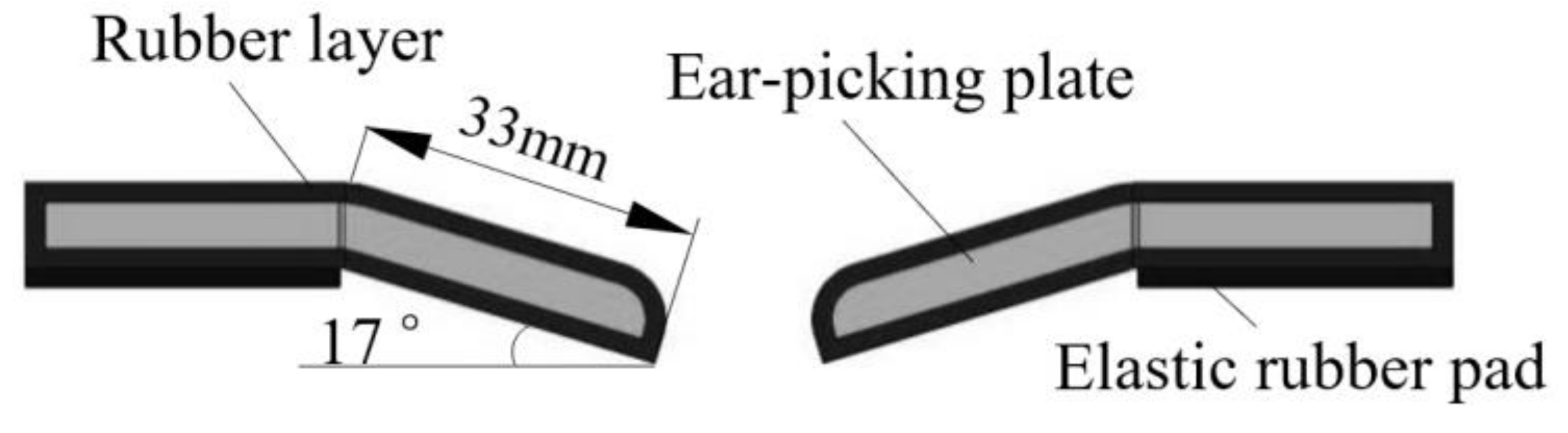
According to the reference [16], increasing the diameter at the point where the ear-picking plate and corn ears come into contact can reduce the instantaneous impact force. However, the flat plate or rounded edge is usually used in the existing corn ear-picking device that includes an ear-picking plate and snapping rolls. It has a small equivalent contact radius and cannot buffer the impact force generated during the ear-picking process. Therefore, the inverted right angle ear-picking plate of this paper has an inclination angle between the edge and horizontal plane. According to ear size measurement data, the bending length of the ear-picking plate is 33 mm, and the angle between the plate and horizon is 17°. Because the force area of the ear in relation to the ear-picking plate is greater than that of the plane plate, the impact force is insufficient to collide kernels. At the same time, two flexible treatments on the ear-picking plate parts have been made to reduce the damage of corn ears during the working process. As shown in Figure 2, the surface layer of the ear-picking plate is treated with glue for 3~5 mm, and an elastic rubber gasket is added under the ear-picking plate to further reduce the impact force received by corn ears in the working process. When the ear-picking device receives the impact of corn ears, the buffering effect of the elastic rubber pad allows it to convert the impact force of corn ears into the potential energy of the elastic rubber pad. The elastic rubber pad returns to its original shape after corn ears are picked, reducing kernels damage.
2.1.2. Structure Design of Snapping Rolls
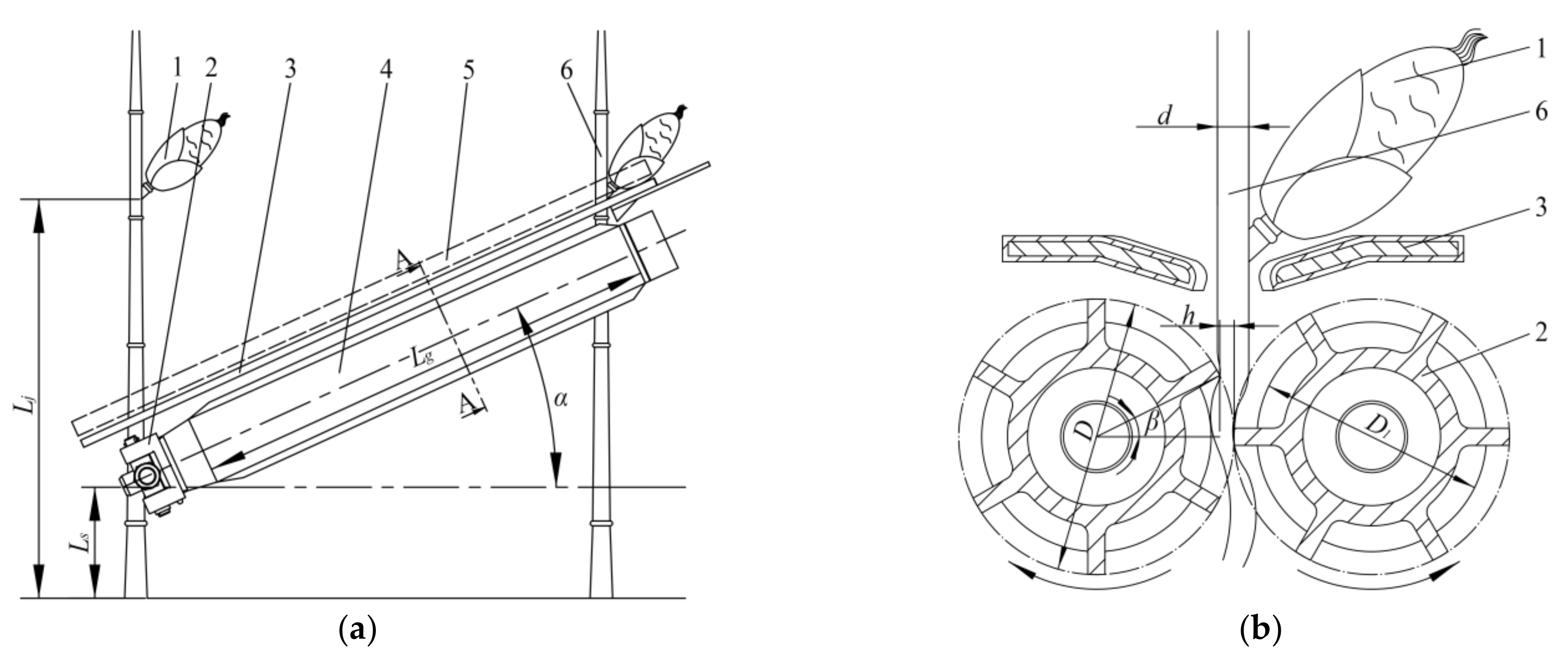
Snapping rolls are welded with ribs on the surface in combination with processing technology to ensure the continuity of the pulling stalk process and improve working efficiency. The snapping rolls have a six-ribbed structure that increases the diameter of the roller [17,18], which can improve the ability of the snapping rolls to grab stalk, and the working principle of the ear-picking device is shown in Figure 3.
When calculating the actual working length of snapping rolls, it should be noted that it can adjust to different corn varieties’ height at corn ear setting, avoiding the phenomenon of snapping rolls pulling two corn plants at the same time.
According to Figure 3, the length Lg is satisfied by the following equation:
where Lj is the ear height of corn plant, mm; Ls is the height of the center line in front of snapping rolls above ground, mm; Lg is the working length of snapping rolls, mm; α is the angle between snapping rolls and horizontal plane, (°).
According to information collected and sorted from the mainly promoted breeding corn in the Huanghuaihai region of China, the height Lj is 700~1100 mm, the height Ls is 300~500 mm, and the angle α is 25~35° when corns are harvested [19]. It can be seen from Equation (1) that the length of snapping rolls is 328~725 mm. When snapping rolls are installed obliquely, and the length is less than 400 mm, the ear-picking effect is not sui. Combined with the overall structure of the machine, the length Lg is selected as 550 mm, which can satisfy the corn breeding harvest of various varieties and growth.
The compression ratio of stalks by the snapping rolls ‘i’ is described as the following equation:
where d is the diameter of the stalk at corn ear, mm; h is the working gap of snapping rolls, mm.
The gripping force produced by snapping rolls will not be able to pick off corn ears if the compression ratio is too small, and the stalk will be prone to breakage if the compression ratio is too high. According to the references [20,21], the best compression ratio is 0.5~0.7, and the corn plant has suitable trafficability when the gap between snapping rolls is 1/2~1/3 of the stalk diameter. Through measurement, the diameter d is 16.1~26.8 mm, and the average value is 21.45 mm. Therefore, the working gap h is set to 10 mm.
The outer diameter D and the diameter D1 can be expressed as the following equation:
where D is the outer diameter of snapping rolls, mm; D1 is the diameter of snapping rolls drum, mm; β is the grabbing angle of snapping rolls to the stalk, (°).
In the expected state, the rib on the one snapping roll moves to the lowest position when the rib on the other snapping roll just touches the stalk. On snapping rolls, six ribs are evenly distributed, and the angle of two adjacent ribs is 60°, then β ≈ 30°. Substitute the working gap h and the average diameter d into Equations (3) and (4). The outer diameter D is 85 mm, and the diameter D1 is 75 mm.
2.1.3. Structure Design of Cleaning System
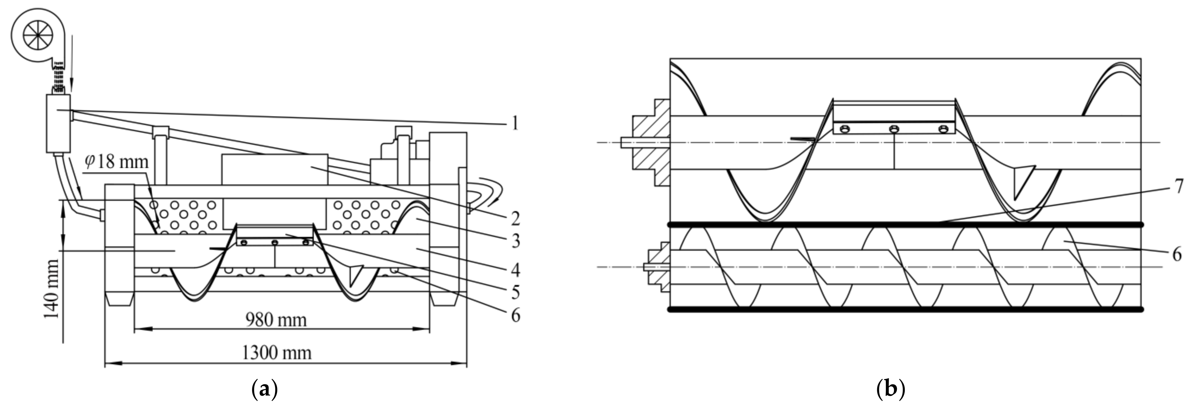
A type of ear-conveying auger with kernel removal function is designed to meet the self-purification agronomic requirements of corn plot harvesters. The structure is shown in Figure 4, including a pneumatically assisted seed cleaning system, auger discharge port, auger blades, ear-conveying auger, scrapers, sieve hole cleaning device, and auger-type kernel recovery devices. The auger rotational speed is 267 r/min, which can fit the input amount of ear-picking device. A centrifugal fan with a rotational speed of 860 r/min and a maximum wind force of 0.36 m3/s is used in the system. The fan’s air outlet is fitted with a pneumatic assisted system that allows the cleaning wind size to be adjusted in real-time according to the harvesting operation.
The ear-conveying auger and the auger-type kernel recovery device are driven by the hydraulic motor to rotate, and the auger transports ears and bracts upwards to the ear lifter. The rubber is wrapped around the edge of the auger blade, which could not only reduce the collision force of corn ears but also eliminate the gap between the auger blade and the bottom of the auger. The inner wall of the auger channel is designed as a streamlined diversion surface with a sieve hole at the bottom. When a plot is harvested, a small number of kernels left in the conveying process will be removed by a sieve hole and lateral pneumatic assisted kernel cleaning system, and the kernels will fall into the kernel recovery device through the sieve hole. A kernel storage box is attached to one end of the auger-type kernel recovery device. After cleaning, the extra kernels will be poured out to prevent mixing between different plots and ensure self-purification of corn harvest in the plot.
2.2. Structure Design of Threshing Device
As shown in Figure 5, the threshing device is composed of a dual-axial flow threshing drum, concave sieve, clutch adjusting device, spiral cleaning device, fan, vibration sieve, etc.
In the threshing chamber, corn ears are threshed by the blow, friction, and rubbing of the dual-axial flow threshing drum, concave sieve, and cover plate. The removed kernels, bracts, and part of broken cores pass through the holes of the concave sieve and fall into a vibrating sieve via an inclined guide plate, while the rear fan blows impurities out of the machine via wind force, completing the first cleaning. A spiral cleaning device at the feeding end of the second threshing chamber is designed to lead a small number of impurities and entrained kernels out of the threshing chamber and fall into a vibrating sieve via the wind force of the front fan to complete the second cleaning. Vibrating separation of kernels and impurities is realized by shaking the sieve under the rotation of the crank, and kernels fall into the unloading port for pneumatic conveying. The kernels and remaining impurities are transported to the zone-bagging device, where the lighter impurities are blown out of the upper part of the zone-bagging device, completing the third cleaning. After harvesting a plot, the machine stops moving forward and continues the wind cleaning operation until the entire threshing device achieves self-purification.
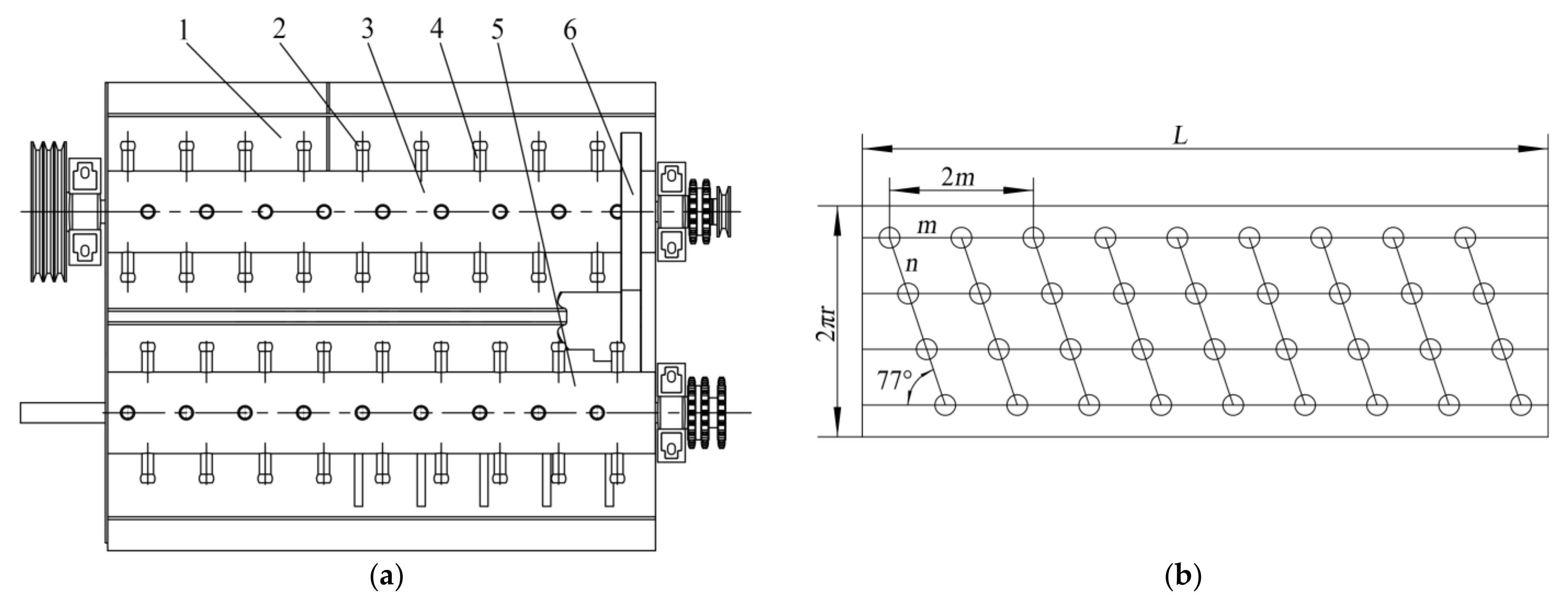
2.2.1. Structure Design of Threshing Drum
The function of the threshing drum is to separate the kernels by beating them, and its structure directly affects the extraction effect of kernels [22,23,24,25]. This paper uses a dual-axial flow threshing drum with a rubber sleeve is provided on the top of each threshing element to reduce the non-threshing and breakage rates in the breeding harvest. The drum speed is low in the front and high in the back, with a speed ratio of 1:2. Figure 6a shows the model and expansion scheme for the threshing element, which uses a hemispherical spike-tooth and spiral arrangement on the threshing shaft. A single drum consists primarily of a drum body and four rows of spike-teeth, with each row of spike-teeth consisting of nine threshing units evenly spaced on each line. So as to lessen the impact on corn.
The feed quantity should be the main design basis of the threshing drum. Because this threshing device is installed on a 2-row corn kernel plot harvester, it should meet the initial setting parameter of 2.5~4 kg/s of the harvester’s feed quantity. Then the drum length L is described as the following equation:
where q is the feed quantity, kg/s; q0 is the allowable feed quantity per unit length, which is 3~4 (kg/s·m) for the combined harvester.
Substituting the data into Equation (5) will get the drum length L as 0.625~1.33 m, according to the overall design requirements of the whole machine and drum, take L = 960 mm. Figure 6b shows an expanded view of the threshing drum. In the figure, m is the distance between two adjacent teeth on the same axis, and n is the arc length of two adjacent teeth on the same spiral line. In order to increase the threshing time and beat frequency in the threshing chamber, the threshing teeth on the same axis should satisfy that m is less than the length of corn ears and n is greater than the length of corn ears. Equation (6) exists and is described as follows:
where l is the length of corn ears, mm.
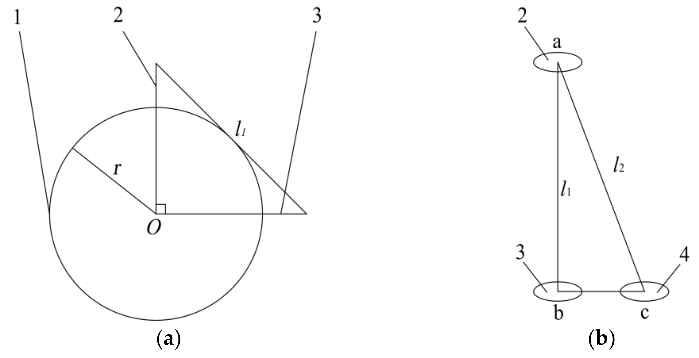
In order to satisfy the axial pushing effect of the threshing drum on corn ears, it is necessary to analyze the distance between two adjacent teeth on the same spiral line. The mathematical model diagram is shown in Figure 7.
Assuming that the shortest length of threshing teeth is x, it should satisfy Equation (7) and is described as follows:
where l1 is the shortest distance between two teeth tangent to drum body on the same section, mm; l2 is the distance between two teeth tangent to the drum body on the same spiral line, mm; r is the radius of the drum, mm.
According to the corn ears length of the plot (l is 175 mm) and the actual working conditions of the harvester, the radius r is selected as 80 mm and m is 100 mm, and the shortest length x of threshing teeth is 42.47 mm by Equation (7). The length of the threshing teeth is 45 mm.
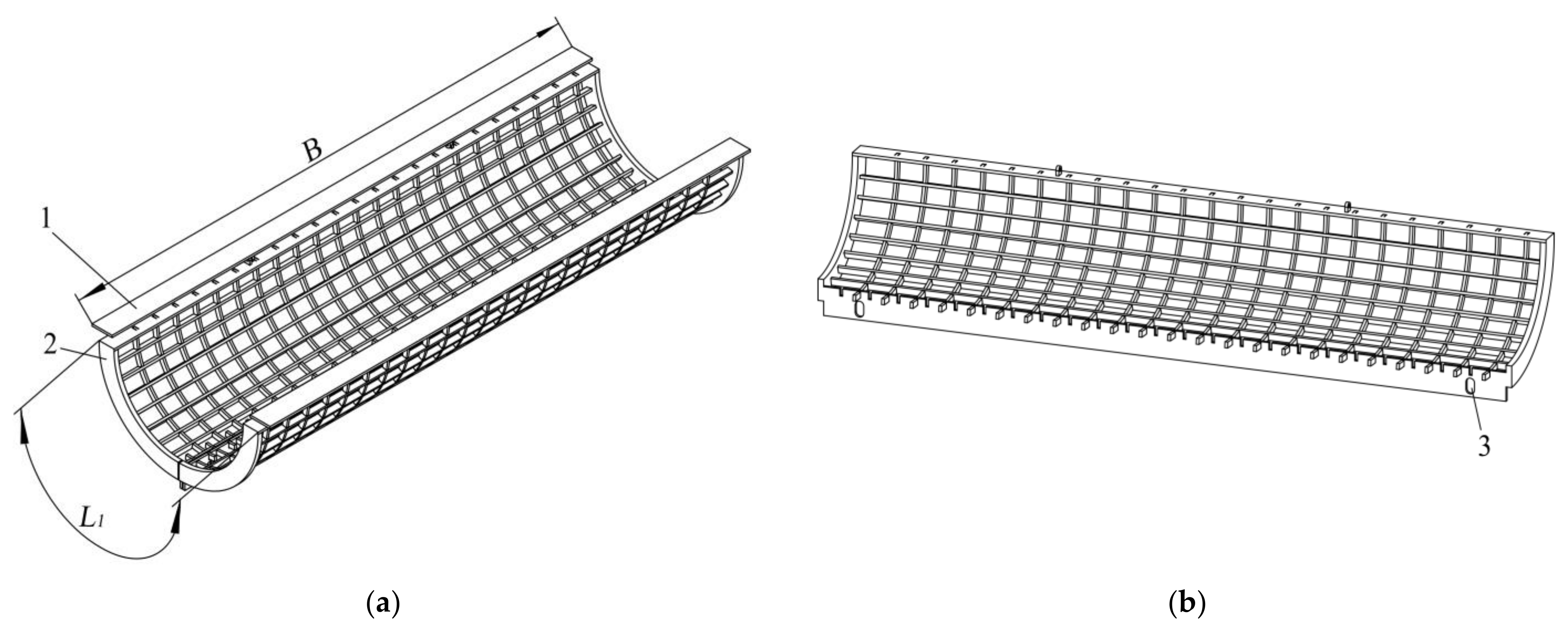
2.2.2. Structure Design of Concave Sieve
The concave sieve is the main threshing component [26,27]. As shown in Figure 8, the concave sieve is grid-type in order to meet the requirements of self-purification during the harvesting of corn kernels in the plot. In order to improve the adaptability of different varieties of harvest, the upper part of the concave plate screen is equipped with a cylindrical pin to enable rotation, and the lower part is drilled with a slot-shaped hole, which is adjusted and fixed by a stud. The bars are 8 mm wide, which have a 30 mm gap between them, and each radial bar extends 20 mm. When the gap between the corncob and vibrating screen is adjusted, the corncob will not fall into the vibrating screen below. Increase the gap after harvesting a plot so that the corn kernels, corn cobs, and impurities in the threshing chamber are cleaned up, and the seeds do not mix when harvesting the next plot.
The concave sieve is in direct contact with the ears of corn during the threshing process, which aids in the shedding of the kernels. The equation of concave sieve area A with respect to arc length L1 is as follows:
where B is the width of concave sieve, mm; L1 is the arc length of concave sieve, mm; q is the feed quantity, kg/s; ε is the ratio of kernels fed into crops; qa is the allowable feed quantity per unit concave sieve area when ε was 0.4, the combine harvester takes 5~8.
The wrap angle δ of concave sieve should satisfy Equation (9) and is described as follows:
Among them, the width B is equal to the length L, which is 960 mm, and the range of arc length L1 can be calculated as 360 mm ≤ L1 ≤ 830 mm. The higher the arc length, the stronger the threshing ability, but the power consumption and the arc length wrap angle will also increase. The wrap angle is mostly 90°~120°, under the premise of satisfying the work quality, take L1 = 500 mm, and put the data into Equation (9) to obtain the wrap angle δ = 120°.
3. Materials and Methods
As shown in Figure 9, firstly, select evaluation indicators and factors according to the analysis and related requirements, and then use the quadratic regression orthogonal combination design experiment to carry out the field test so as to obtain the regression equation corresponding to evaluation indicators. The regression equation is used to analyze the influence of factors and optimize the index, and finally, the optimized value is verified and compared with the corresponding field test.
3.1. Force Analysis of Threshing Device
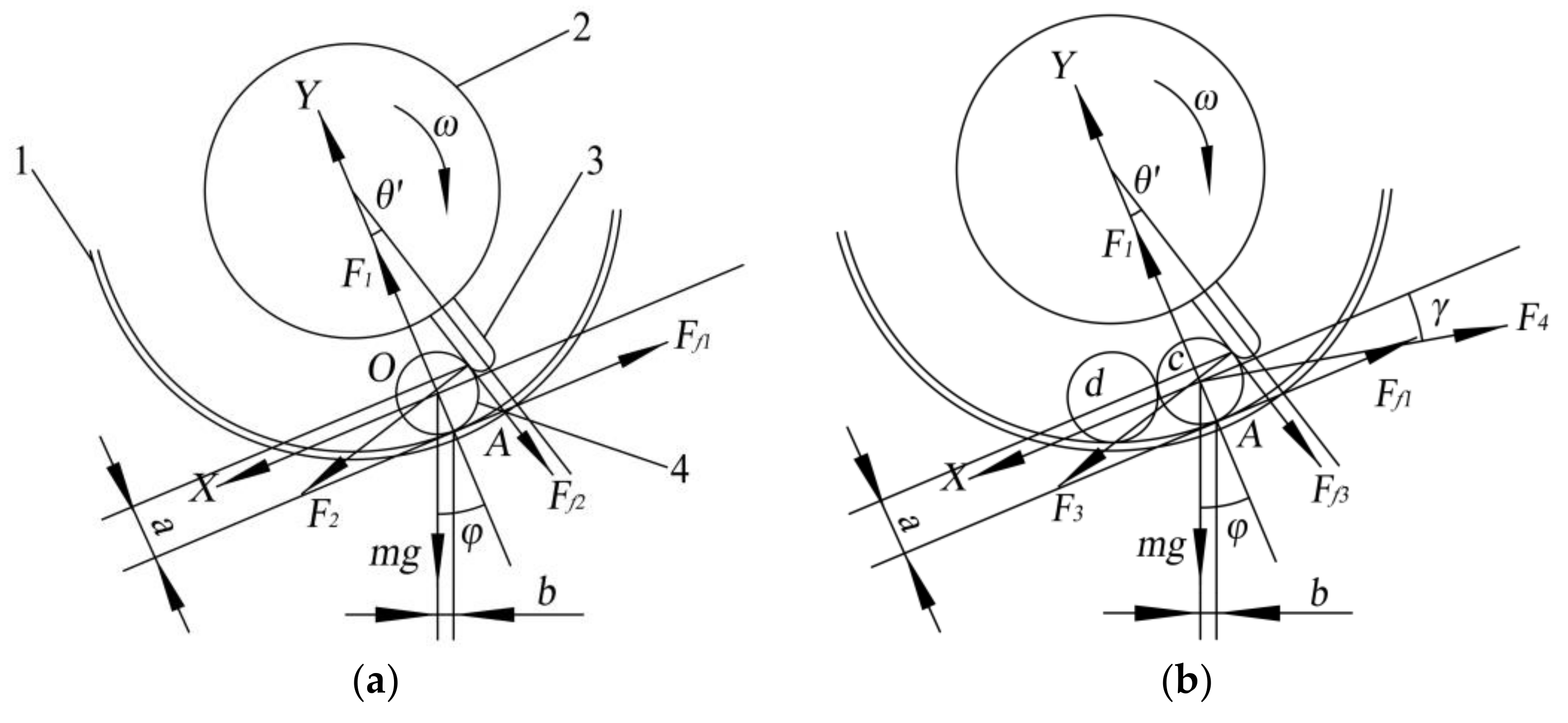
The force involved in threshing corn ears is more complicated. The single corn ear threshing process is taken as the research object under the ideal state of low feed rate, the force on the ear is translated to the barycenter, and the force analysis is shown in Figure 10a without considering the torque. Using the barycenter position O of corn ears as the origin, the connecting line between the barycenter of corn ears and the center of the threshing drum is the Y axis, the movement direction of corn is the positive direction of the X axis, and A is the contact point where the ear meets the concave sieve.
Then the force acting on the ear with low feeding should satisfy the following equation:
where F1 is the supporting force of concave sieve on the ear, N; F2 is the impact of threshing teeth on the ear, N; μ1 is the friction coefficient between the ear and concave sieve; usually, μ1 is 0.059; μ2 is the friction coefficient between the ear and threshing teeth; usually, μ2 is 0.102 [28]; Ff1 is the friction between the ear and concave sieve, Ff1 = μ1F1, N; Ff2 is the friction between the ear and threshing teeth, Ff2 = μ2F2, N; θ′ is the included angle between Y axis and the axis of the threshing tooth, °; usually, θ′ is 17 °; φ is the angle between Y axis and the direction of gravity, °; r is ear radius, mm; ω is the angular speed of the drum, rad/s.
According to Equations (10) and (11), the force F2 is simplified by Equation (12):
The equation of the moment of the force acting on the ear to point A is as follows:
where a is the distance from the intersection of the ear and the threshing tooth to the concave sieve, mm; b is the distance from the barycenter of the ear to the concave sieve, mm.
From the above mechanical analysis, it can be seen that the ear force with low feeding is mainly related to the impact force F2, the included angle θ′, and the length a, etc. Therefore, the drum speed and threshing gap have an effect on the damage of kernels.
Under the ideal state of high-feeding, take ear c as the research object, and its force analysis is shown in Figure 10b, then the Equations (14) and (15) exists and is described as follow:
where F3 is the impact force of threshing tooth on the ear c, N; F4 is the pressure of ear d on ear c, N; Ff3 is the friction force between ear c and threshing tooth, Ff3 = μ2F3, N; γ is the angle between the pressure F4 and the friction force Ff1, °.
According to Equations (10)~(15), the force F3 is simplified by Equation (16):
According to Equations (12) and (16), the impact of threshing teeth on the ear can be express by Equation (17):
According to Equation (17), when 0° < γ < 90°, F3 − F2 > 0. Therefore, the feed quantity increases, then the impact force of threshing teeth on the ear increases under the condition of a certain drum speed.
3.2. Key Performance Parameters of Corn Plot Kernel Harvester
3.2.1. Breakage Rate
In the measurement area, extract kernels from kernel outlet at least 2000 g after threshing and cleaning. Pick out the machine-damaged, cracked, and broken kernels and weigh the quality of damaged kernels and the total mass of sample kernels, respectively. Their test method in this research followed the National Standards of China, Corn combine harvester (GB/T 21962-2020). The breakage rate is calculated according to Equation (18), and it is described as follows:
where Zs is the breaking rate, %; Ws is the mass of damaged kernels, g; Wi is the total mass of sample kernels, g.
3.2.2. Non-Threshing Rate
The quality of non-threshing kernels accounts for a percentage of the total quality of kernels after one plot has been harvested and threshing has been completed. The non-threshing rate is calculated according to Equation (19), which is described as follows:
where Sw is the non-threshing rate, %; Ww is the quality of kernels that are not decontaminated, g; W is the total mass of kernels, g.
3.3. Key Experimental Factors of Corn Plot Kernel Harvester
From the above analysis, the factors that affect kernels breakage during the harvesting process of corn plot are drum speed, threshing gap, and feed quantity. In order to facilitate calculation, the forward speed of the machine is used instead of feed quantity.
3.3.1. Speed of Threshing Drum
The speed of the threshing drum is closely related to the breakage rate, which directly affects the impact, friction, and rubbing force of ears during threshing [29]. The front drum is faster than the back drum in this article. Therefore, the second threshing drum speed is selected as the test factor for the convenience of measurement. If the speed of the threshing drum is too fast, the impact force increased, resulting in an increase in the rate of kernel breakage and broken straw impurities. The burden of cleaning is greatly increased, and the power consumption will increase as well. If the speed is too low, the impact force will be insufficient, and kernels will not be removed. Meanwhile, the material staying and rubbing repeatedly in the threshing chamber for a long time will also increase the breakage rate. Therefore, the adjustment range of the second drum speed is set to 500~800 r/min.
3.3.2. Threshing Gap
The threshing gap is the minimum distance between the top of the drum threshing tooth and the concave sieve, and its size is related to the diameter of the ears. The gap is narrower than the average diameter of ears generally so that the ear can be squeezed and rubbed during the feeding process [30]. The basic characteristic parameters of Zhengdan 958 ears are shown in Table 1. Based on the statistical results in Table 1 and the overall structure of the machine, the adjustment range of the threshing gap is set to 20~40 mm.
3.3.3. Forward Speed
While increasing the feed rate can achieve higher harvest efficiency and shorten the working time, the quality of the operation will suffer, resulting in an increase in the rate of corn breakage during harvest, which affects the quality of the harvest. The relational function equation between the feeding amount and the forward speed of the harvester is described as follow:
where q is the feed quantity, Kg/s; n is the number of corn rows; m is the quality of single corn, Kg; v is the forward speed of the harvester, m/s; s is the distance between corn plants, m.
According to the planting mode of the test base, the feed quantity is proposed to be 1~2.5 kg/s, and the adjustment range of forward speed is 0.5~1.26 m/s based on Equation (20).
3.4. Materials of Field Test
The test site was conducted in Zhangpan Town, Xuchang County, Henan Province. The test plot was 100 × 70 m in size, with corn rows 800 mm apart, plants 350 mm apart, the plant lodging rate was less than 5%, and the minimum scion height was 1100 mm. The corn variety used in the field test was Zhengdan 958, and its basic characteristic parameters are listed in Table 1.
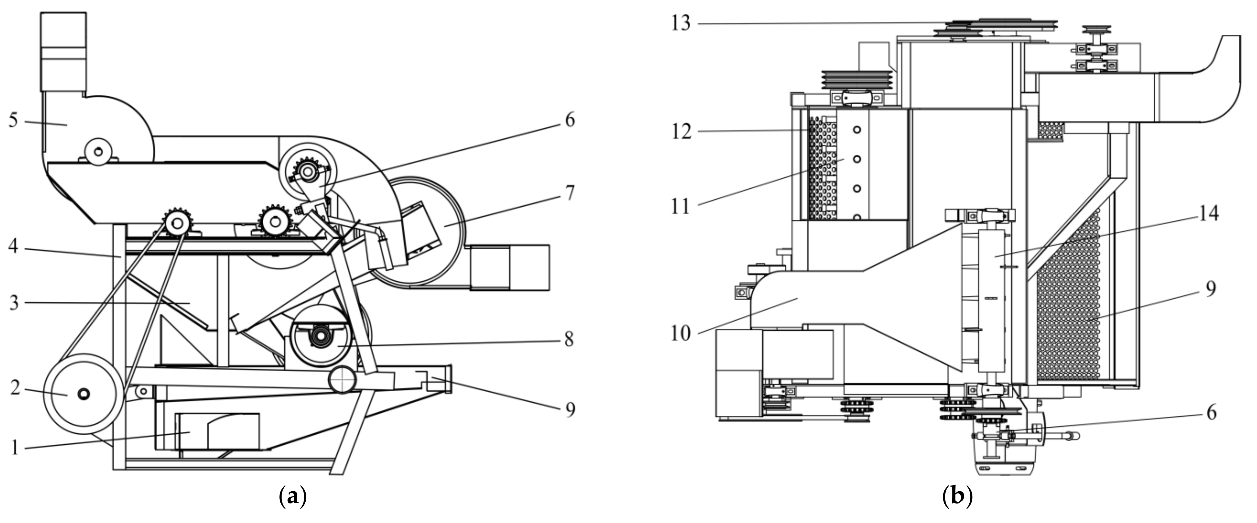
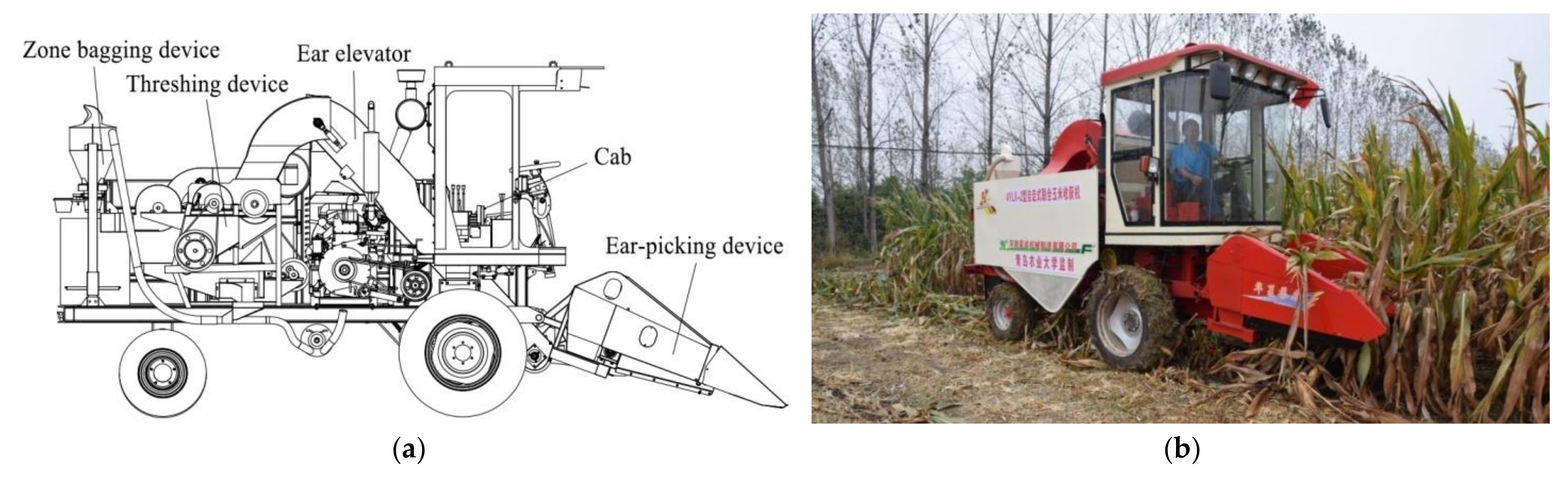
As shown in Figure 11, the flexible gap self-adjusting ear-picking plate and the dual-axial flow threshing device were installed to a 4YZL-2 corn plot kernel harvester (Henan Haofeng Machinery Manufacturing Co., Ltd., Henan, China), which can complete ear-picking lifting, threshing, and collection in one operation. The lossless harvest of corn plots and the realization of no mixed kernels between plots are the technical features. The harvester has extremely high technical requirements, and the working parameters are shown in Table 2.
3.5. Methods of Field Test
Combined with the above analysis and the actual working conditions of the prototype, taking the forward speed z1, the second threshing drum speed z2, and the threshing gap z3 as the experimental factors. The experimental factors and levels are shown in Table 3.
This test adopts a three-factor quadratic regression orthogonal combination design and sets three zero-level tests (m0 = 3), which can be obtained r2 = 1.831 [31]. The experimental factors need to be coded before the test, and the coding method is shown in Table 4.
The formula for centralizing the quadratic term is described as follows:
The breakage rate y1 and the non-threshing rate y2 has been used as the test evaluating indexes. The total number of tests is 17, and each group of tests is repeated 3 times to obtain the average value, and the test scheme and results are shown in Table 5.
4. Results and Discussion
4.1. Results of Filed Test
4.2. Regression Analysis of Filed Test
As shown in Table 6, the p-value of lack of fit Pl is 0.2691, the p-value of residuals model PR is 0.00014, indicating that the regression equation of the experimental index fits well. Taking α = 0.05 as the significance level, the primary term x1, x2, x3, the square term x12, and the interaction term x1x3 have extremely significant effects, while other factors have no significant effects. After removing the insignificant terms, the regression equation of the dimensionless code value of the breakage rate is obtained as:
From Equation (22), it can be seen that the influence order of experimental factors on breakage rate is that threshing clearance, forward speed, and second threshing cylinder speed. According to Table 4, the actual regression equation of breakage rate was obtained after sorting:
As shown in Table 7, the p-value of lack of fit Pl is 0.1894, the p-value of residuals model PR is 0.00052, indicating that the regression equation of the experimental index fits well. Taking α = 0.05 as the significance level, the primary term x1, x2, and x3 have highly significant effects, the square term x12 and the interaction term x1x3 have significant effects, while other factors have no significant effects. After removing the insignificant terms, the regression equation of the dimensionless code value of the non-threshing rate is obtained as:
From Equation (24), it can be seen that the influence order of experimental factors on the non-threshing rate is that forward speed, threshing clearance, and second threshing cylinder speed. According to Table 4, the actual regression equation of non-threshing rate was obtained after sorting:
The regression analysis results are shown in Table 8. The correlation coefficient R of the breakage rate y1 and the non-threshing rate y2 reached 0.9856 and 0.9786, which indicating that there is a strong linear relationship between experimental factors and test indicators in the regression model. The coefficient of determination R2 of the breakage rate y1 and the non-threshing rate y2 reached 0.9714 and 0.9576, which indicating that the regression model has a high degree of fit. In order to avoid the limitation of coefficient of determination R2, and adjusted coefficient of determination Adj R2 is obtained. It shows that the adjusted coefficient of determination of breakage rate y1 is 0.9668, which means the independent variables in the model can explain the 96.68% variation of breakage rate. Similarly, the adjusted coefficient of determination of non-threshing rate y2 is 0.9503, which means the independent variables in the model can explain the 95.03% variation of the non-threshing rate. Durbin-Watson statistic satisfies the conditions of 1 < d < 3 at the same time, so the test data have strong reliability.
The distribution of test measured and fitted values for the two regression models are shown in Figure 13. The test measured values are represented by the blue line, while the sample fitted values are represented by the orange line. It can be seen that the two values are very well matched.
4.3. Interaction Analysis of Filed Test
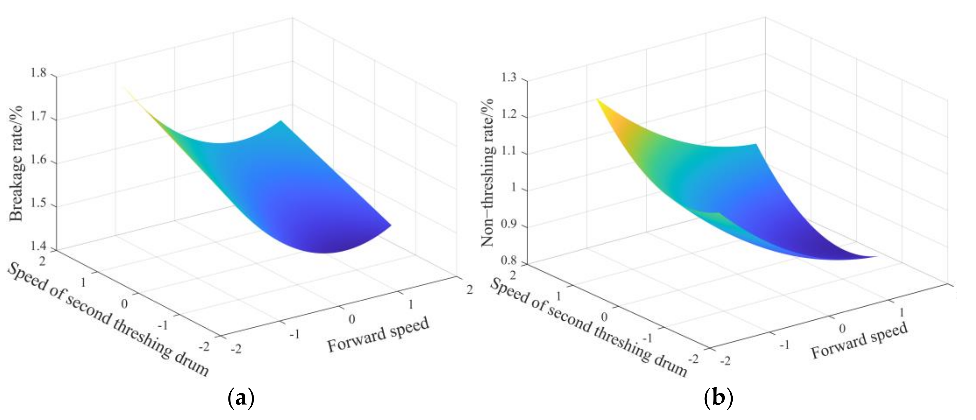
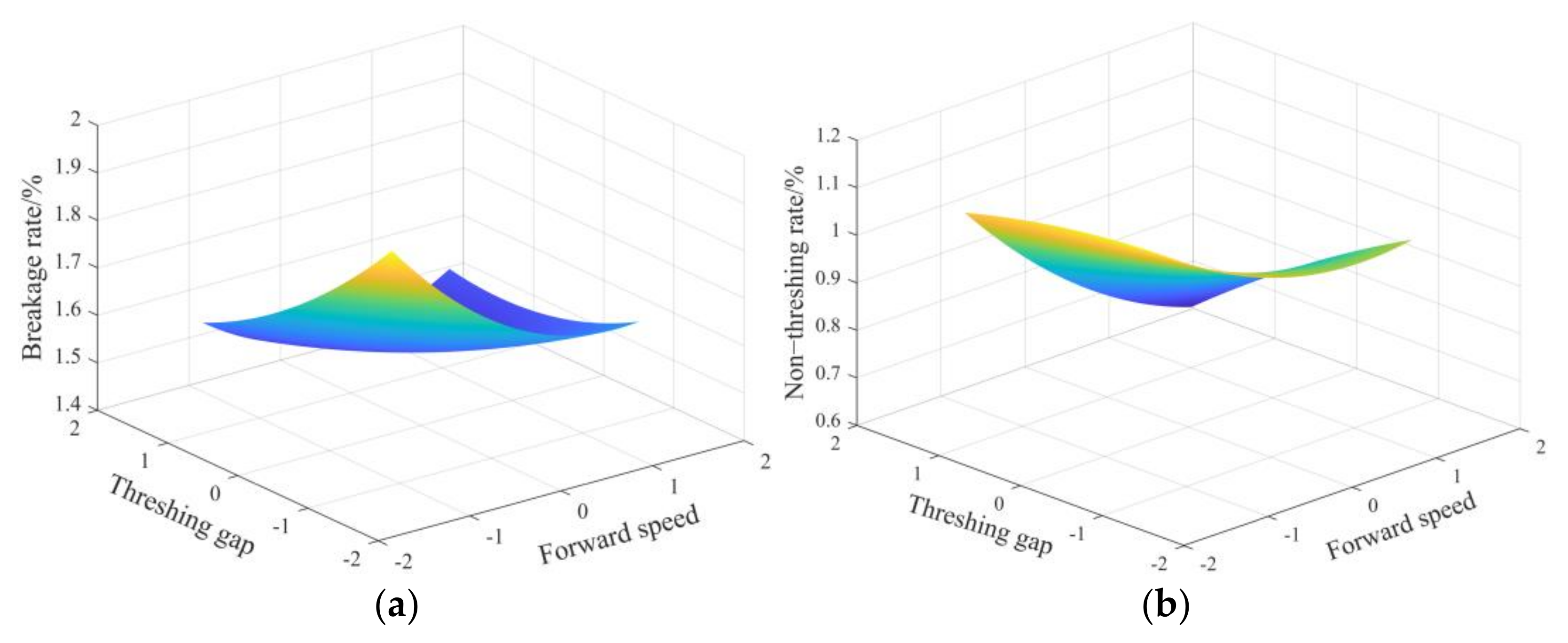
In order to obtain the influence law of the experimental factors on each test index more intuitively, study the interaction effect of the other two factors by fixing a certain factor at zero levels, and the regression equation is transformed into a three-dimensional contour map through MATLAB, which are shown in Figure 14, Figure 15 and Figure 16.
4.3.1. Interaction Analysis between Forward Speed and Second Threshing Speed Drum
Figure 14a shows that the breakage rate decreases at first and then increases as the forward speed increase. This is because when the feed amount is low, the strike force and strikes number of nail teeth are limited. After that, according to Equation (17), when 0° < γ < 90°, the impact force of threshing gear under high feed amount F3 is greater than the impact force of the threshing gear under low feed amount F2. The feeding amount increases with the forward speed increase, and the impact force of threshing teeth will also increase, resulting in a higher breakage rate. Therefore, there will be a double change phenomenon. In order to ensure a small and reasonable breakage rate, the forward speed can be controlled within the range of 0.5~0.88 m·s−1.
Duane et al. [32] showed that the kernel damage increased with increased kernel velocity and was related more to this than any of the other factors tested. With the increase in threshing drum speed, the overall breakage rate shows an upward trend. Increasing the speed of the threshing drum will increase the hitting frequency of threshing teeth and the number of impacts and rubbing, which increases the breakage rate. The drum speed should be controlled at a minimum of 500 r·min−1. These findings are consistent with the findings of Di et al. [15]. It can be concluded that the effect of forward speed on the breakage rate is significantly higher than that of the threshing drum speed from the response cloud map.
Figure 14b shows that the non-threshing rate presents a downward trend as the forward speed increases. This is due to the increase in feed quantity, which increases the chances of contact between drum and ear. As the speed of the threshing drum increases, the non-threshing rate decreases first and then increases. This is because the drum speed increases, allowing for more contact opportunities. It is known from Equation (12) that the impact of threshing teeth on ear F2 decreases when the angular speed of drum ω increases, thereby lowering the non-threshing rate. It can be concluded that the forward speed has a higher impact on the non-threshing rate than the speed of the threshing drum from the response cloud map.
4.3.2. Interaction Analysis between Forward Speed and Threshing Gap
Figure 15a shows that the increase in the threshing gap causes the breakage rate to decrease significantly. This is because as the threshing gap widens, the effect of threshing elements on the ear was weakened, the grain crushing rate was reduced, the mutual squeezing and rubbing effect between ear was weakened, resulting in the non-threshing rate was increased. This is similar to the findings of Chen et al. [29]. The breakage rate decreases at first then increases as the forward speed increases. This is because, with the increase in the feeding amount, the ears cannot move in the axial direction in time, which will cause accumulation. It can be concluded that the effect of the threshing gap on the breakage rate is slightly higher than the forward speed from the response cloud map.
Figure 15b shows that the non-threshing rate increases slightly as the threshing gap widens and decreases significantly as the forward speed increases, and the response speed of forward speed in the map is faster than the threshing gap. When the feeding amount is large, there are more ears in the gap between the threshing drum and concave plate, and the threshing elements are in full contact with the corn ears to improve the non-threshing rate [33]. It can be concluded that the effect of the threshing gap on the non-threshing rate is lower than the forward speed from the response cloud map.
4.3.3. Interaction Analysis between Second Threshing Drum Speed and Threshing Gap
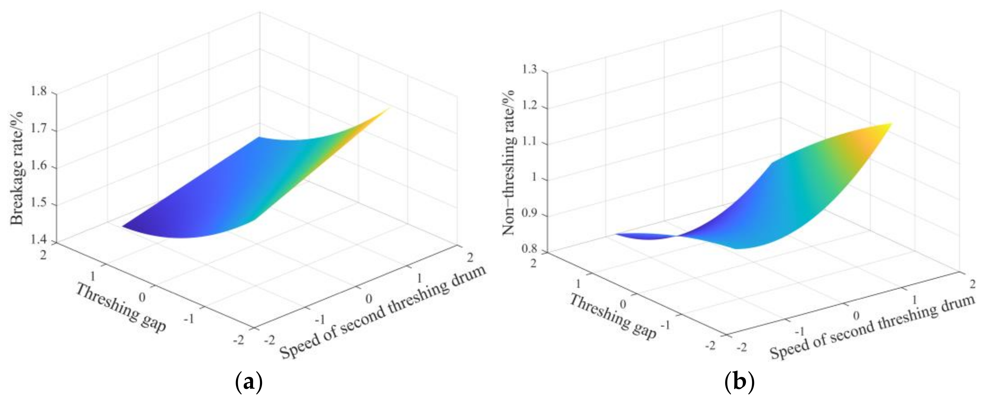
Figure 16a shows that the breakage rate decreases significantly as the threshing gap widens and increases as the threshing drum speed increases. This is because when the feeding amount is constant, the threshing gap increases and the beating frequency of corn will not increase rapidly with the increase in drum speed. It can be concluded that the effect of the threshing gap on the breakage rate is slightly higher than the speed of the threshing drum from the response cloud map.
Figure 16b shows that when the forward speed is consistent, the non-threshing rate decreases at first and then increases as the threshing drum speed increases and decreases slightly as the threshing gap widens, but the response speed of the threshing gap in the map is much slower than the threshing drum speed. This is because with the increase in drum speed, the threshing efficiency of the drum was also improved, and the retention time of corn in the threshing chamber was reduced, resulting in the increase in non-threshing rate [30]. It can be concluded that the effect of threshing drum speed on the non-threshing rate is significantly higher than the threshing gap from the response cloud map.
4.4. Performance Optimization of Filed Test
According to the requirements of corn plot kernel harvesting, the minimum breakage rate and non-threshing rate of kernels should be met during harvest. Create the objective function for the two indicators above, and substitute the obtained regression model into the function. The objective function and constraint conditions are described as follows:
Using MATLAB to optimize the parameters, the optimal value is obtained as the forward speed is 0.61 m/s, the speed of the threshing drum is 500 r/min, and the threshing gap is 40 mm. The verification test uses Zhengdan 958, which is the same variety as the regression orthogonal combination design test. The number of tests is three times, and the average value is taken. The results are shown in Table 9. The test results show that in the optimal parameters test, the field test validation value is close to the theoretical value.
5. Conclusions
(1) Based on the existing ear-picking mechanism, the basic parameters of the ear-picking device are theoretically studied by sorting out and collecting information on the main popularized breeding corn to ensure the reasonable and reliability of the design. Combining with the structural characteristics of corn plot kernel harvester, a flexible gap self-adjusting ear-picking device and a dual-axial flow corn threshing device were optimized through a pneumatically assisted seed cleaning system and three times of cleaning to realize the non-mixed harvest of kernels between plots.
(2) Through the mechanical analysis of corn ears, it is concluded that the factors affecting kernel damage were drum speed, threshing gap, and feed quantity. Combining the actual working conditions of the prototype, it is determined that the forward speed of the unit varies from 0.4 to 1.0 m/s, the speed of the threshing drum varies from 300 to 500 r/min, and the threshing gap is arbitrarily adjustable within the range of 20~40 mm.
(3) The field test carried out the quadratic regression orthogonal combination design by taking the breakage rate and the non-threshing rate as the test evaluating indexes. The test data were analyzed to produce a quadratic regression model between the breakage rate and the non-threshing rate. Through the significance analysis of regression coefficients, it is known that the regression model has a high degree of fit. Meanwhile, the distribution of test measured and fitted values for the two regression models are very well matched.
(4) Furthermore, through the interactive analysis of three factors, it can be concluded that the forward speed has a significant impact on the breakage rate and the non-threshing rate. The threshing gap has a greater impact on the breakage rate than the speed of the threshing drum. The effect of the threshing drum speed on the non-threshing rate is greater than the effect of the threshing gap. Then the optimal operating parameters of the machine are calculated by optimization, which showed that the forward speed was 0.61 m/s, the speed of the threshing drum was 500 r/min, and the threshing gap was 40 mm. More importantly, the minimum breakage rate and non-threshing rate were 1.47% and 0.89%, respectively in the field validation test.
6. Patents
The flexible gap self-adjusting ear-picking device and dual-axial flow corn threshing device reported in this manuscript have been applied for patents in China (Application No. CN108293421A).
Author Contributions
Conceptualization, R.Y. and D.C.; Data curation, D.C. and X.Z.; Formal analysis, R.Y. and D.C.; Funding acquisition, S.S.; Investigation, R.Y., X.Z. and Z.P.; Methodology, R.Y. and D.C.; Project administration, S.S.; Resources, R.Y. and X.Z.; Software, R.Y. and D.C.; Supervision, S.S.; Validation, R.Y., D.C., X.Z. and Z.P.; Visualization, R.Y. and X.Z.; Writing—original draft, R.Y. and D.C.; Writing—review and editing, R.Y. and D.C. All authors have read and agreed to the published version of the manuscript.
Funding
This work was financially supported by the research and development of seed breeding technology and equipment (Grant No. 2017YFD0701200), which is the National Key Research and Development Project of China.
Institutional Review Board Statement
Not applicable.
Informed Consent Statement
Not applicable.
Data Availability Statement
The data presented in this study are available on-demand from the second author at ([email protected]).
Acknowledgments
This work was financially supported by the National Key Research and Development Project of China (research and development of seed breeding technology and equipment, 2017YFD0701200). We thank Guoying Li for its fund and investigation assistance during the preparation of this manuscript. All supports and assistance are sincerely appreciated.
Conflicts of Interest
The authors declare no conflict of interest.
References
- Zhu, M.; Chen, H.; Li, Y. Investigation and development analysis of seed industry mechanization in China. Int. J. Agr. Biol. Eng. 2015, 31, 1–7. [Google Scholar]
- Qin, X.; Feng, F.; Li, Y.; Xu, S.; Siddique, K.H.M.; Liao, Y. Maize yield improvements in China: Past trends and future directions. Plant. Breed. 2016, 135, 166–176. [Google Scholar] [CrossRef]
- Huang, M.; Zou, Y. Integrating mechanization with agronomy and breeding to ensure food security in China. Field Crops Res. 2018, 224, 22–27. [Google Scholar] [CrossRef]
- Hou, L.; Wang, K.; Wang, Y.; Li, L.; Ming, B.; Xie, R. In-field harvest loss of mechanically-harvested maize kernel and affecting factors in China. Int. J. Agric. Biol. Eng. 2021, 14, 29–37. [Google Scholar] [CrossRef]
- Babić, L.; Radojèin, M.; Pavkov, I.; Babić, M.; Turan, J.; Zoranović, M.; Stanišić, S. Physical properties and compression loading behaviour of corn seed. Int. Agrophysics 2013, 27, 119–126. [Google Scholar] [CrossRef]
- Volkovas, V.; Petkevičius, S.; Špokas, L. Establishment of maize kernel elasticity on the basis of impact load. Mechanika 2006, 6, 64–67. [Google Scholar]
- Petre, I.M. Combine Harvesters Theory, Modeling and Design; Taylor & Francis Group: Boca Raton, FL, USA, 2016. [Google Scholar]
- Pickard, G.E. Laboratory studies in corn combining. Agric. Eng. 1955, 36, 792–794. [Google Scholar]
- Srivastava, A.K.; Herum, F.L.; Stevens, K.K. Impact parameters related to physical damage to corn kernel. Trans. ASABE 1976, 19, 1147–1151. [Google Scholar] [CrossRef]
- Voicu, G.; Cǎsǎndroiu, T.; Stan, G. Using the dimensional analysis for a mathematical model to predict the seeds losses at the cleaning system of the cereals harvesting combines. U.P.B. Sci. 2007, 69, 29–39. [Google Scholar]
- Fu, Q.; Fu, J.; Chen, Z.; Han, L.; Ren, L. Effect of impact parameters and moisture content on kernel loss during corn snapping. Int. Agrophys. 2019, 33, 493–502. [Google Scholar] [CrossRef]
- Geng, A.; Yang, J.; Zhang, J.; Zhang, Z.; Yang, Q.; Li, R. Influence factor analysis of mechanical damage on corn ear picking. Trans. Chin. Soc. Agric. Eng. 2016, 32, 56–62. [Google Scholar]
- Li, X.; Wu, K. Design and Experiment of Bionic Discrete Devices Based on Corn Threshing System. Chem. Eng. Trans. 2016, 51, 127–132. [Google Scholar] [CrossRef]
- Li, X.; Du, Y.; Guo, J.; Mao, E. Design, Simulation, and Test of a New Threshing Cylinder for High Moisture Content Corn. Appl. Sci. 2020, 10, 4925. [Google Scholar] [CrossRef]
- Di, Z.; Cui, Z.; Zhang, H.; Zhou, J.; Zhang, M.; Bu, L. Design and experiment of rasp bar and nail tooth combined axial flow corn threshing cylinder. Int. J. Agric. Biol. Eng. 2018, 34, 28–34. [Google Scholar]
- Li, K. Design and Experimental Study on Gap-Adjustable Combined Ear-Picking Mechanism of Corn; China Agricultural University: Beijing, China, 2018. [Google Scholar]
- Du, Y.; Mao, E.; Zhu, Z.; Wang, X.; Yue, X.; Li, X. Design and Experiment of Two row Corn Harvester Header. Trans. Chin. Soc. Agric. Mach. 2013, 44 (Supp2), 22–26. [Google Scholar]
- He, J. Biomimetic Surfaces of Snapping Rolls with Lower Damage Action and Simulation of No-Row Feed-in Mechanism of Maiz Harvesters; Jilin University: Jilin, China, 2007. [Google Scholar]
- Zhang, Z.; Chi, R.; Du, Y.; Pan, X.; Dong, N.; Xie, B. Experiments and modeling of mechanism analysis of maize picking loss. Int. J. Agric. Biol. Eng. 2021, 14, 11–19. [Google Scholar] [CrossRef]
- Zhang, Z. Study on a New Corn Combine Harvester Header for Reaping both Corn Stalk and Spike; China Agricultural University: Beijing, China, 2018. [Google Scholar]
- Xin, S. Study on the Mechanism and Key Technology of Corn Ear Picking with Vertical Roller; Gansu Agricultural University: Lanzhou, China, 2020. [Google Scholar]
- Li, X.; Xiong, S.; Du, Z.; Geng, L.; Ji, J. Design and experiment on floating corn single panicle threshing device. Int. J. Agric. Biol. Eng. 2017, 48, 104–111. [Google Scholar] [CrossRef]
- Yi, S.; Tao, G.; Mao, X. Comparative experiment on the distribution regularities of threshed mixtures for two types of axial flow threshing and separating installation. Int. J. Agr. Biol. Eng. 2008, 24, 154–156. [Google Scholar]
- Wan, X.; Liao, Q.; Xu, Y.; Yuan, J.; Li, H. Design and evaluation of cyclone separation cleaning devices usding a conical sieve for rape combine harvesters. Appl. Eng. Agric. 2018, 34, 677–686. [Google Scholar] [CrossRef]
- Yang, L.; Wang, W.; Wang, M.; Zhang, H.; Hou, M. Structural Dynamics of Corn Threshing Drum Based on Computer Simulation Technology. Wireless Pers Commun. 2018, 102, 701–711. [Google Scholar] [CrossRef]
- Gao, L.; Zhang, S.; Chen, R.; Yang, D. Design and experiment on soybean breeding thresher of double feeding roller and combined threshing cylinder. Trans. Chin. Soc. Agric. Mach. 2015, 46, 112–118. [Google Scholar] [CrossRef]
- Yang, D.; Jiang, D.; Shen, Y.; Gao, L.; Wan, L.; Wang, J. Design and Test on Soybean Seed Thresher with Tangential-axial Flow Double-roller. Trans. Chin. Soc. Agric. Mach. 2017, 48, 102–110. [Google Scholar] [CrossRef]
- Tang, H. Design and Mechanism Analysis of Ripple Surface Pickup Finger Maize Precision Seed Metering Device; Dongbei Agricultural University: Shenyang, China, 2018. [Google Scholar]
- Chen, M.; Xu, G.; Wang, C.; Diao, P.; Zhang, Y.; Niu, G. Design and Experiment of Roller-type Combined Longitudinal Axial Flow Flexible Threshing and Separating Device for Corn. Trans. Chin. Soc. Agric. Mach. 2020, 51, 123–131. [Google Scholar] [CrossRef]
- Yang, L.; Wang, W.; Zhang, H.; Li, L.; Wang, M.; Hou, M. Improved design and bench test based on tangential flow-transverse axial flow maize threshing system. Int. J. Agric. Biol. Eng. 2018, 34, 35–43. [Google Scholar] [CrossRef]
- He, Y. Experimental Design and Analysis; Chemical Industry Press: Beijing, China, 2013. [Google Scholar]
- Keller, D.; Converse, H.; Hodges, T.; Chung, D. Corn kernel damage due to high velocity impact. Trans. ASAE 1972, 12, 330–331. [Google Scholar] [CrossRef]
- Wang, Z.; Wang, Z.; Zhang, Y.; Yan, W.; Chi, Y.; Liu, C. Design and test of longitudinal axial flexible hammer-claw corn thresher. Trans. Chin. Soc. Agric. Mach. 2020, 51, 109–117. [Google Scholar]
Figure 1.
Installation and working diagram of gap self-adjusting ear-picking plate.

Figure 2.
Structural scheme of V-shaped ear-picking plate.

Figure 3.
Working scheme of snapping rolls. 1. Corn ear 2. Snapping rolls 3. Ear-picking plate 4. Snapping rolls gap adjustment device 5. Gathering chain 6. Corn stalk. (a) Working scheme, (b) A-A Cross section scheme. Note: Lj is the ear height of corn plant, mm; Ls is the height of the center line in front of snapping rolls above ground, mm; Lg is the working length of snapping rolls, mm; α is the angle between snapping rolls and horizontal plane, (°); d is the diameter of the stalk at corn ear, mm; h is the working gap of snapping rolls, mm; D is the outer diameter of snapping rolls, mm; D1 is the diameter of snapping rolls drum, mm; β is the grabbing angle of snapping rolls to the stalk, (°).

Figure 4.
Cleaning system scheme of ear-picking device. 1. Pneumatic assisted seed cleaning system 2. Auger discharge port 3. Auger blades 4. Ear-conveying auger 5. Scraper 6. Sieve hole cleaning device 7. Auger-type kernel recovery device. (a) Top view, (b) Main view.
Figure 4.
Cleaning system scheme of ear-picking device. 1. Pneumatic assisted seed cleaning system 2. Auger discharge port 3. Auger blades 4. Ear-conveying auger 5. Scraper 6. Sieve hole cleaning device 7. Auger-type kernel recovery device. (a) Top view, (b) Main view.

Figure 5.
Structural scheme of threshing device. 1. kernel discharge port 2. Crank drive wheel 3. Inclined guide plate 4. Frame 5. Front fan 6. Clutch adjustment device 7. Rear fan 8. Core discharging device 9. Vibrating sieve 10. Front fan air supply channel 11. Threshing roller 12. Concave plate screen 13. Drive wheel 14. Spiral impurity removal device. (a) Main view, (b) Top view.

Figure 6.
Model and expansion scheme of threshing drum. 1. Feeding inlet 2. Rubber 3. First drum body 4. Threshing tooth 5. Ear guide plate 6. Second drum body. (a) Structure scheme, (b) Cylinder unfolded view. Note: m is the distance between two adjacent teeth on the same axis, mm; n is the arc length of two adjacent teeth on the same spiral line, mm; L is the drum length, mm.

Figure 7.
Mathematical model diagram. 1. Threshing drum 2. Threshing gear a 3. Virtual threshing gear b 4. Threshing gear c. (a) Cylinder section view, (b) Distribution of threshing teeth. Note: l1 is the shortest distance between two teeth tangent to drum body on the same section, mm; l2 is the distance between two teeth tangent to the drum body on the same spiral line, mm; r is the radius of the drum, mm.

Figure 8.
Concave sieve model diagram. 1. Fixed plate 2. Movable sieve 3. Slot hole. (a) Concave Screen Combination Diagram, (b) Concave sieve split diagram. Note: B is the width of concave, mm; L1 is the arc length of concave, mm.
Figure 8.
Concave sieve model diagram. 1. Fixed plate 2. Movable sieve 3. Slot hole. (a) Concave Screen Combination Diagram, (b) Concave sieve split diagram. Note: B is the width of concave, mm; L1 is the arc length of concave, mm.

Figure 9.
Flowchart of materials and methods.

Figure 10.
Stress analysis of corn. 1. Concave sieve 2. Threshing drum 3. Threshing teeth 4. Corn. (a) Low-feeding ear force diagram, (b) High-feeding ear force diagram. Note: F1 is the supporting force of concave sieve on the ear, N; F2 is the impact of threshing teeth on the ear, N; F3 is the impact force of threshing tooth on ear c, N; F4 is the pressure of ear d on ear c, N; μ1 is the friction coefficient between the ear and concave sieve; μ2 is the friction coefficient between the ear and threshing teeth; Ff1 is the friction between the ear and concave sieve, N; Ff2 is the friction between the ear and threshing teeth, N; Ff3 is the friction force between ear c and threshing tooth, N; θ’ is the included angle between Y axis and the axis of the threshing tooth, °; φ is the angle between Y axis and the direction of gravity, °; γ is the angle between the pressure F4 and the friction force Ff1, °; ω is the angular speed of the drum, rad/s; r is ear radius, mm; a is the distance from the intersection of ear and the threshing tooth to the concave sieve, mm; b is the distance from the barycenter of the ear to the concave sieve, mm.

Figure 11.
Ear-picking device and threshing device with 4YZL-2 corn plot kernel harvester. (a) Structural diagram, (b) Real machine diagram.
Figure 11.
Ear-picking device and threshing device with 4YZL-2 corn plot kernel harvester. (a) Structural diagram, (b) Real machine diagram.

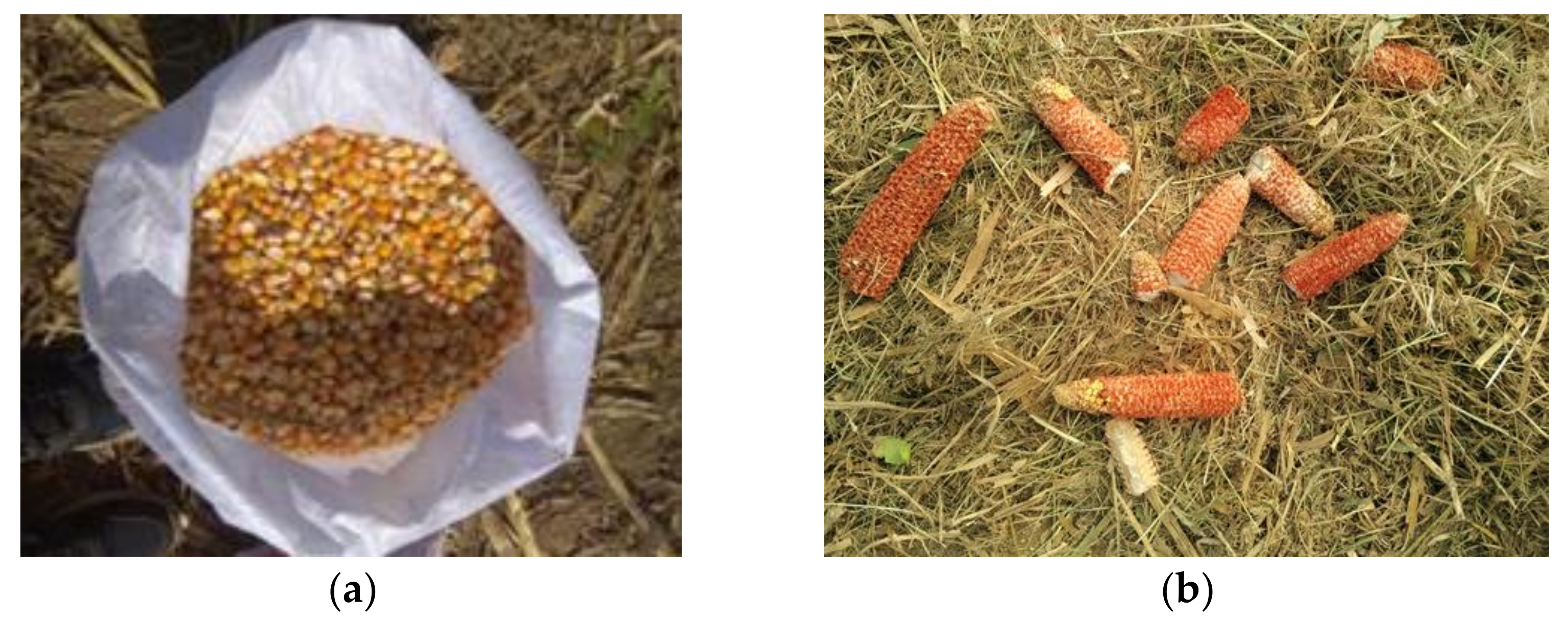
Figure 12.
Presentation of harvest result. (a) Harvested corn grain, (b) threshed corn.

Figure 13.
Distribution of test measured and fitted values. (a) Fitting curve of breakage rate, (b) fitting curve of non-threshing rate.
Figure 13.
Distribution of test measured and fitted values. (a) Fitting curve of breakage rate, (b) fitting curve of non-threshing rate.

Figure 14.
Interaction between the forward speed and the speed of the second threshing drum. (a) Effect on breakage rate, (b) effect on the non-threshing rate.
Figure 14.
Interaction between the forward speed and the speed of the second threshing drum. (a) Effect on breakage rate, (b) effect on the non-threshing rate.

Figure 15.
Interaction between the forward speed and the threshing gap. (a) Effect on breakage rate, (b) effect on the non-threshing rate.
Figure 15.
Interaction between the forward speed and the threshing gap. (a) Effect on breakage rate, (b) effect on the non-threshing rate.

Figure 16.
Interaction between the speed of the second threshing drum and the threshing gap. (a) Effect on breakage rate, (b) effect on the non-threshing rate.
Figure 16.
Interaction between the speed of the second threshing drum and the threshing gap. (a) Effect on breakage rate, (b) effect on the non-threshing rate.


Table 1.
Corn basic characteristic parameters in the plot.
| Parameters | Value |
|---|---|
| Average ear length/mm | 174.36 |
| Average weight per ear/kg | 0.348 |
| Average diameter of large end/mm | 54.2 |
| Average diameter of small end/mm | 35.8 |
| Kernel moisture content/% | 21~26 |
Table 2.
Main technical parameters of plot corn kernel harvester.
| Parameters | Value |
|---|---|
| Structure form | Self-propelled wheel |
| Type of diesel engine | JDM490 |
| Rated power of engine/kW | 37 |
| Rated speed of engine/(r·min−1) | 2400 |
| Vehicle weight/kg | 2600 |
| Harvest rows/row | 2 |
| Minimum ground clearance/mm | 250 |
| Applicable line spacing/mm | 550~650 |
| Size/(mm × mm × mm) | 5200 × 1300 × 2650 |
| Working width/mm | 1200 |
Table 3.
Experimental factors and levels.
| Factors | Forward Speed z1/(m· s−1) | Speed of Second Threshing Drum z2/ (r·min−1) | Threshing Gap z3/mm | |
|---|---|---|---|---|
| Levels | ||||
| 1 | 0.5 | 500 | 20 | |
| 2 | 0.88 | 650 | 30 | |
| 3 | 1.26 | 800 | 40 | |
Table 4.
Coding method of experimental factors.
| Code | Forward Speed Z1/(m· s−1) | Speed of Second Threshing Drum Z2/ (r·min−1) | Threshing Gap Z3/mm | |
|---|---|---|---|---|
| Factors | ||||
| r (Z2j) | 1.26 | 800 | 40 | |
| 1(Z0j + Δj) | 1.16 | 760.86 | 37.39 | |
| 0(Z0j) | 0.88 | 650 | 30 | |
| 1(Z0j − Δj) | 0.6 | 539.14 | 22.61 | |
| −r (Z1j) | 0.50 | 500 | 20 | |
| Δj = (Z2j − Z1j)/2r | 0.28 | 110.86 | 7.39 | |
| xj = (Zj − Z0j)/Δj | x1 = 3.571(z1 − 0.52) | x2 = 0.009(z2 − 650) | x3 = 0.135(z3 − 30) | |
Note: Δj is the minimum change interval of the j-th factor, j = 1, 2, 3; xj is the encoded factor; r is the asterisk arm.
Table 5.
Test program and results by quadratic regression orthogonal combination design.
| Factors | x0 | x1 | x2 | x3 | x1x2 | x1x3 | x2x3 | x12 | x22 | x32 | y1 | y2 | |
|---|---|---|---|---|---|---|---|---|---|---|---|---|---|
| Test | |||||||||||||
| 1 | 1 | 1 | 1 | 1 | 1 | 1 | 1 | 1 | 1 | 1 | 1.54 | 0.83 | |
| 2 | 1 | 1 | 1 | −1 | 1 | −1 | −1 | 1 | 1 | 1 | 1.66 | 1.12 | |
| 3 | 1 | 1 | −1 | 1 | −1 | 1 | −1 | 1 | 1 | 1 | 1.48 | 0.78 | |
| 4 | 1 | 1 | −1 | −1 | −1 | −1 | 1 | 1 | 1 | 1 | 1.55 | 0.95 | |
| 5 | 1 | −1 | 1 | 1 | −1 | −1 | 1 | 1 | 1 | 1 | 1.62 | 1.07 | |
| 6 | 1 | −1 | 1 | −1 | −1 | 1 | −1 | 1 | 1 | 1 | 1.87 | 1.19 | |
| 7 | 1 | −1 | −1 | 1 | 1 | −1 | −1 | 1 | 1 | 1 | 1.53 | 0.98 | |
| 8 | 1 | −1 | −1 | −1 | 1 | 1 | 1 | 1 | 1 | 1 | 1.76 | 1.05 | |
| 9 | 1 | −r | 0 | 0 | 0 | 0 | 0 | r2 | 0 | 0 | 1.69 | 1.13 | |
| 10 | 1 | r | 0 | 0 | 0 | 0 | 0 | r2 | 0 | 0 | 1.59 | 0.81 | |
| 11 | 1 | 0 | −r | 0 | 0 | 0 | 0 | 0 | r2 | 0 | 1.49 | 0.92 | |
| 12 | 1 | 0 | r | 0 | 0 | 0 | 0 | 0 | r2 | 0 | 1.61 | 1.09 | |
| 13 | 1 | 0 | 0 | −r | 0 | 0 | 0 | 0 | 0 | r2 | 1.67 | 0.96 | |
| 14 | 1 | 0 | 0 | r | 0 | 0 | 0 | 0 | 0 | r2 | 1.51 | 0.84 | |
| 15 | 1 | 0 | 0 | 0 | 0 | 0 | 0 | 0 | 0 | 0 | 1.56 | 0.93 | |
| 16 | 1 | 0 | 0 | 0 | 0 | 0 | 0 | 0 | 0 | 0 | 1.57 | 0.91 | |
| 17 | 1 | 0 | 0 | 0 | 0 | 0 | 0 | 0 | 0 | 0 | 1.54 | 0.95 | |
Note: xj is the encoded factor, j = 1, 2, 3; r is the asterisk arm.
Table 6.
Variance analysis for breakage rate.
| Source | Sum of Squares | Degree of Freedom | Mean Square | F Value | p-Value |
|---|---|---|---|---|---|
| x1 | 0.040 | 1 | 0.0402 | 58.98 | 0.00012 ** |
| x2 | 0.024 | 1 | 0.0243 | 35.59 | 0.00056 ** |
| x3 | 0.067 | 1 | 0.0674 | 98.70 | 0.00002 ** |
| x1x2 | 0.0001 | 1 | 0.00011 | 0.165 | 0.69693 |
| x1x3 | 0.011 | 1 | 0.0105 | 15.40 | 0.00572 ** |
| x2x3 | 0.0006 | 1 | 0.00061 | 0.897 | 0.37511 |
| x12 | 0.016 | 1 | 0.0161 | 23.65 | 0.00183 ** |
| x22 | 0.00000004 | 1 | 0.00000004 | 0.00006 | 0.99391 |
| X32 | 0.0032 | 1 | 0.0032 | 4.653 | 0.06791 |
| Regression | 0.163 | 9 | 0.0181 | 26.45 | 0.00014 ** |
| Residuals | 0.0048 | 7 | 0.00068 | / | / |
| Lack of fit | 0.0043 | 5 | 0.00086 | 1.58 | 0.2691 |
| Error | 0.00047 | 2 | 0.00023 | / | / |
| Total | 0.1673 | 16 | / | / | / |
Note: ** indicates highly significant (p ≤ 0.01).
Table 7.
Variance analysis for non-threshing rate.
| Source | Sum of Squares | Degree of Freedom | Mean Square | F Value | p-Value |
|---|---|---|---|---|---|
| x1 | 0.09328 | 1 | 0.0933 | 65.77 | 0.000084 ** |
| x2 | 0.03965 | 1 | 0.0397 | 27.96 | 0.001138 ** |
| x3 | 0.05659 | 1 | 0.0566 | 39.901 | 0.000398 ** |
| x1x2 | 0.000013 | 1 | 0.000013 | 0.0088 | 0.9278 |
| x1x3 | 0.00911 | 1 | 0.0091 | 6.425 | 0.03896 * |
| x2x3 | 0.00361 | 1 | 0.0036 | 2.547 | 0.1545 |
| x12 | 0.00575 | 1 | 0.0058 | 4.051 | 0.08401 |
| x22 | 0.0157 | 1 | 0.0157 | 11.07 | 0.01264 * |
| X32 | 0.00054 | 1 | 0.00054 | 0.3793 | 0.5575 |
| Regression | 0.22425 | 9 | 0.0249 | 17.568 | 0.00052 ** |
| Residuals | 0.00993 | 7 | 0.00141 | / | / |
| Lack of fit | 0.00913 | 5 | 0.00183 | 4.564 | 0.1894 |
| Error | 0.0008 | 2 | 0.0004 | / | / |
| Total | 0.2342 | 16 | / | / | / |
Note: ** indicates highly significant (p ≤ 0.01); * indicates significant (0.01 ≤ p ≤ 0.05).
Table 8.
Significance analysis of regression coefficient on the test results.
| Inspection Items | y1 | y2 |
|---|---|---|
| R | 0.9856 | 0.9786 |
| R2 | 0.9714 | 0.9576 |
| Adj R2 | 0.9668 | 0.9503 |
| S | 0.0261 | 0.0377 |
| Durbin-Watson statistic | 2.7176 (1 < d < 3) | 2.1973 (1 < d < 3) |
Table 9.
Optimum parameters test results.
| Breaking Rate y1/% | Non-Threshing Rate y2/% | Fmin/% | |
|---|---|---|---|
| Theoretical value | 1.45 | 0.82 | 2.27 |
| Field test validation value | 1.47 | 0.89 | 2.36 |
Publisher’s Note: MDPI stays neutral with regard to jurisdictional claims in published maps and institutional affiliations. |
© 2021 by the authors. Licensee MDPI, Basel, Switzerland. This article is an open access article distributed under the terms and conditions of the Creative Commons Attribution (CC BY) license (https://creativecommons.org/licenses/by/4.0/).
Share and Cite
MDPI and ACS Style
Yang, R.; Chen, D.; Zha, X.; Pan, Z.; Shang, S. Optimization Design and Experiment of Ear-Picking and Threshing Devices of Corn Plot Kernel Harvester. Agriculture 2021, 11, 904. https://doi.org/10.3390/agriculture11090904
AMA Style
Yang R, Chen D, Zha X, Pan Z, Shang S. Optimization Design and Experiment of Ear-Picking and Threshing Devices of Corn Plot Kernel Harvester. Agriculture. 2021; 11(9):904. https://doi.org/10.3390/agriculture11090904
Chicago/Turabian StyleYang, Ranbing, Dongquan Chen, Xiantao Zha, Zhiguo Pan, and Shuqi Shang. 2021. "Optimization Design and Experiment of Ear-Picking and Threshing Devices of Corn Plot Kernel Harvester" Agriculture 11, no. 9: 904. https://doi.org/10.3390/agriculture11090904
Note that from the first issue of 2016, this journal uses article numbers instead of page numbers. See further details here.