Autonomous and Safe Navigation of Mobile Robots in Vineyard with Smooth Collision Avoidance

Abstract

In recent years, autonomous robots have extensively been used to automate several vineyard tasks. Autonomous navigation is an indispensable component of such field robots. Autonomous and safe navigation has been well studied in indoor environments and many algorithms have been proposed. However, unlike structured indoor environments, vineyards pose special challenges for robot navigation. Particularly, safe robot navigation is crucial to avoid damaging the grapes. In this regard, we propose an algorithm that enables autonomous and safe robot navigation in vineyards. The proposed algorithm relies on data from a Lidar sensor and does not require a GPS. In addition, the proposed algorithm can avoid dynamic obstacles in the vineyard while smoothing the robot’s trajectories. The curvature of the trajectories can be controlled, keeping a safe distance from both the crop and the dynamic obstacles. We have tested the algorithm in both a simulation and with robots in an actual vineyard. The results show that the robot can safely navigate the lanes of the vineyard and smoothly avoid dynamic obstacles such as moving people without abruptly stopping or executing sharp turns. The algorithm performs in real-time and can easily be integrated into robots deployed in vineyards.

1. Introduction

In recent years, autonomous robots have extensively been used to lower the burden of farmers. In several countries, demographic changes are a major factor behind this trend. For instance, the proposed research was carried out in vineyards in Japan where there is an increase in the old-age population in Japan. Moreover, the number of farmers is steadily decreasing. This makes it difficult to sustain agriculture and related industries. Figure 1a shows the population and average age of farmers in Japan from year 2000 to year 2014 based on a survey by Japan’s Ministry of Agriculture, Forestry and Fisheries (MAFF) [1]. It is clear that the farming population in Japan is steadily declining from 2.4 million in the year 2000 to 1.68 million in the year 2014. On the contrary, it is also evident that the average age of the farmers is steadily increasing. The average farmer’s age in Japan was 62.2 years in the year 2000, which was already an alarming situation. The situation worsened in the year 2014 when the average farmer’s age reached 66.8 years. Figure 1b shows the gender wise comparison of the farming population in Japan. A similar trend can be seen from this figure. Most of the male and female farming population is concentrated around the 65∼69 years age-group. What is alarming is that a significant farming population can be seen in the 70∼74 years age-group and above. In Japan, the younger population is reluctant to engage in laborious farming activities and instead prefer office work. The situation becomes graver as Japan faces fierce competition from low-cost products from abroad, and is often forced to either reduce costs or to find a way to add value to their products. This trend is seen in other countries too, where there is also a problem of shortage of farmers. It should be noted that apart from the aging population, there are several other factors that necessitate the incorporation of field robots in agriculture. However, since this research was conducted in Japan, which faces severe demographic challenges, this effect has been emphasized.

A major concern with agricultural activities is that they involve mostly labor-intensive tasks. Such tasks are difficult to perform for old people. Robotic technology has a large potential to support agricultural activities by automating many tasks. Such efforts to lower the burden of farmers by automating tasks to reduce labor are highly desirable as they directly lead to an increase in production and sustainable agriculture. In recent years, autonomous agricultural robots have shown remarkable progress to support different activities autonomously or semi-autonomously. However, many challenges still remain as open problems. In order to autonomously perform tasks in the farms, autonomous navigation is a quintessential component of robots. Generally, GPS is used in outdoor farms to localize the robot and enable it to navigate autonomously. Lidars have also been used extensively. Both GPS and Lidar have their own merits and demerits. The cost of these sensors generally vary a lot depending on various factors such as precision, accuracy and robustness. Accurate GPS (centimeter level precision) is expensive. On the other hand, an inexpensive GPS generally has an error in the order of tens or hundreds of centimeters, which is unfit for robot navigation in a vineyard with a lane width of approximately 2.5 m. Three-dimensional Lidars such as Velodyne VLP-16 and VLP-32 are expensive; however, a 2D Lidar is relatively cheaper with good accuracy. Since our research is focused in Japan, the QZSS (Quasi-Zenith Satellite) system, also called ‘Michibiki’, that launched in 2018 is worth mentioning [2,3]. The QZSS is a four-satellite regional time transfer system and a satellite-based augmentation system development by the Japanese government to enhance the United States-operated Global Positioning System in the Asia-Oceania regions, with a focus on Japan. QZSS is a Japanese satellite positioning system composed mainly of satellites in quasi-zenith orbits (QZO). QZSS (Michibiki) has been operated as a four-satellite constellation from November 2018, and three satellites are visible at all times from locations in the Asia-Oceania region. QZSS can be used in an integrated way with GPS, ensuring a sufficient number of satellites for stable, high-precision positioning. Although the price of these sensors is currently high, the cost is expected to decrease in the future. To keep the current cost of the system down, the developed system mainly relies on Lidar sensors. However, integration of GPS is feasible for better results.

To navigate accurately, a robot needs a map of the environment, which marks the obstacles and free areas. It also needs to localize itself on the map. Then, given the start and goal locations, the robot can navigate through the free areas avoiding the obstacles using path planning algorithms. To realize this, mobile robots are equipped with sensors to perceive the external world. These include sensors such as Lidar, cameras, RGBD (RGB color and Depth) sensors, IMU, GPS, and external sensors [4]. In addition, robots are also equipped with a SLAM (Simultaneous Localization and Mapping) [5,6] module, which uses data from these sensors to build a map of the environment and localize its position in the map. The SLAM module extracts features from the sensor data, which are used as landmarks to accurately build the map and localize itself in it. Failure to robustly extract landmarks results in a wrong map and localization errors, which eventually affects tasks performed by the mobile robot.

Robotics for vineyards have been well studied for different applications in both academics and industries [7]. Both single [8,9] and multi-robot scenarios [10] for localization with trunk recognition have been proposed. Other researchers have focused on autonomous pruning [11] and total yield estimation [12,13]. Similarly, managing the irrigation in vineyards has been studied in [14]. In all these works, autonomous safe navigation is assumed to be available with the robot and algorithms have been proposed [15]. In many works, robotics approaches have been coupled with IoT-based approaches for vineyards [16,17,18,19,20,21,22,23,24]. It should be noted that all of these works implicitly depend on the navigation module of a mobile robot. Particularly, tasks such as vineyard monitoring [23,25,26,27] cannot be successfully executed without safe autonomous navigation. Dynamic obstacles must also be considered for navigation. A wireless sensor network for vineyard monitoring that uses image processing is proposed in [25].

Figure 2 shows the standing of the proposed research (yellow block) in vineyard field robots. As mentioned above, researchers have focused on automation of several tasks in vineyards such as grape harvesting, weed removal, monitoring, and yield-estimation. From a system development point of view, it can be suggested that these are high level applications, which assume the availability of certain core modules. The core modules include 2D and 3D mapping, robot’s localization, robot control, and path planning with obstacle avoidance. The core modules support the high level applications. For example, the robotic grape harvesting application requires a 3D map, which marks the grapes and stem that comes from a mapping module. Similarly, the robot needs to localize itself in the vineyard to perform harvesting at appropriate areas. This requires a localization module. Moreover, a path planning module is required to move the robot while avoiding obstacles to appropriate areas of the vineyard that need harvesting. Similarly, a path planning module with obstacle avoidance is indispensable for weed removal, monitoring, and yield estimation applications. Our previous work [28] focused on the development of a monitoring system for vineyards using mobile robots. Vineyards have large areas and manual monitoring consumes a lot of time and effort. Hence, autonomous mobile robots equipped with side facing monocular cameras were used to record the images and transmit them to the farmers who can monitor the vineyard on their mobile or tablet. The recorded images are labeled by area and pillar numbers for the farmer to monitor specific areas of the vineyard. This inherently depends on a reliable navigation module. For yield estimation applications, appropriate sensors such as multispectral and hyperspectral cameras can be fixed on the robot. Similarly, a manipulator and gripper mechanism can be mounted on the robot for harvesting. Weed removal may require a special cutting mechanism. However, the core module for the mobile base on which these sensors will be mounted will remain unchanged.

This work is an extension of our previous work [28], which focused on developing a monitoring system for vineyards using autonomous mobile robots. Our previous work relied on detecting pillars from cameras through image processing. However, it had the drawbacks that pillar detection relied on good light conditions, and only the pillars adjacent to the robot were detected with no depth information. Moreover, the focus was on numbering the pillars and generating semantic data for monitoring purposes. However, this paper focuses on the navigational aspects of the autonomous mobile robots in vineyards. Moreover, it uses Lidar data to extract the position of pillars in the vineyard for navigation. In addition, Lidar sensor data are also used to estimate the position of obstacles in the vicinity. It should be noted that cameras can also be used to detect the pillars and the obstacles. Monocular cameras have also been used for obstacle detection in many works [29,30]. The accuracy of monocular camera-based depth estimation is typically lower than direct estimation from Lidar or stereo cameras for real-time scenarios. Recently, depth estimation from monocular cameras using deep learning techniques has been proposed in [31,32,33]. However, the accuracy of depth estimation in such methods is lower than direct estimation using Lidar. Monocular cameras have the advantage of full-body pose and orientation recognition, which can be useful for obstacle avoidance. Hence, a combination of cameras and Lidar sensors is expected to produce better results and is considered for future works. At the current stage, the proposed work uses a straightforward method of pillar and obstacle detection using a Lidar sensor.

The rest of the paper is organized as follows. Section 2 explains the algorithm for pillar detection from a Lidar sensor. Section 3 explains the algorithm for trajectory smoothing while avoiding the obstacles. Section 4 highlights the results of experiments in an actual vineyard. Finally, Section 5 concludes this paper.

2. Pillar Detection from Lidar Sensor Data

Navigation requires precise localization of the robot in the map. In order to localize the robot in the vineyard, robust feature detection is very essential. Many outdoor robots use GPS for localization. However, GPS is expensive and its induction adds to the overall cost of the system. Accurate localization without GPS requires extraction of robust features in the vineyard. Cameras can be used for feature localization, however, they suffer from the problems of occlusion and changes in pixel intensities at different times of the day. In this regard, this research proposes to use only Lidar for feature extraction. Most of the vineyards have stationary pillars, which are fixed to support the grapes and the plant. These pillars are good features to track for navigation in the vineyard.

The algorithm for pillar detection from Lidar is given in Algorithm 1. The algorithm directly applies a symmetric derivative on Lidar data d as,

$$\begin{array}{c}\hfill L^{\prime }={\displaystyle \frac{d[i+1]-d[i-1]}{2}},\end{array}$$

(1)

where i is the $i\mathrm{th}$ Lidar data point. The symmetric derivative ($L^{\prime }$) gives a falling and rising edge from which the pillar is localized in the center position.

Algorithm 1: Safe Navigation with Feature (Pillar) Detection from Lidar

This is explained in Figure 3, which shows three different scenarios of pillar detection in a vineyard. Figure 3a shows the simplest case with one pillar. The blue lines indicate the Lidar rays given as $\mathrm{ray\_idx}$ in Algorithm 1. Figure 3b shows the symmetric derivative ($L^{\prime }$ in red) of the Lidar data (d in blue). The derivative has two peaks on the left and right side indicated as $\mathrm{L}$ and $\mathrm{R}$, respectively. The center of the two peaks marks the position of the pillar.

Similarly, Figure 3c shows the scenarios of two pillars on the left and right side of the Lidar sensor. The symmetric derivative is shown in Figure 3d. The derivative has two rising and falling edges indicated as (${\mathrm{L}}_1,{\mathrm{R}}_1$) and (${\mathrm{L}}_2,{\mathrm{R}}_2$), respectively. The two pillars are detected in the centers of these edges.

Figure 3e shows the scenarios of two pillars in which one pillar (${\mathrm{P}}_2$) is behind another pillar (${\mathrm{P}}_1$) in the front. Here, the pillar ${\mathrm{P}}_1$ needs to be detected. The symmetric derivative is shown in Figure 3f. The derivative has two falling edges and one rising edge indicated as (${\mathrm{L}}_1,{\mathrm{L}}_2$) and ($\mathrm{R}$), respectively. The two pillars are detected in the center of the edges ${\mathrm{L}}_2$ and $\mathrm{R}$.

Figure 3g–i shows the aforementioned three scenarios in an actual vineyard. Figure 3g shows the scenario in which there is only one pillar on the left side of the robot. This is a particular section of the vineyard where there is no vegetation on the right hand side. Hence, detection of a single pillar is also important, and the robot must navigate while tracking the single pillar. Figure 3h shows the scenario of two pillars on the left and right side of the Lidar sensor. Similarly, Figure 3i shows the actual scenario of two pillars in which one pillar is behind another pillar in the front. Here, the pillar in the front needs to be detected.

It should be noted that the presence of obstacles (ex. weeds) in front of the pillars could induce noise in the Lidar data and the symmetric derivative could contain short falling and rising edges. However, this noise can easily be filtered by setting a threshold value, such that only those edges are recorded whose strength lies above and below a certain threshold. The threshold is shown in Figure 3 in the derivative graphs as dotted blue lines. The value of the threshold is determined empirically. Figure 4 shows the picture of actual weed in a vineyard. Although the type of weed may vary from region to region, in the context of the current research undertaken in a vineyard in Japan, the maximum height of the weeds was approximately 20 cm, while the lidar was set at a greater height. Hence, noise from the weeds did not affect the accuracy of pillar detection. Although it should be mentioned that very tall weed will adversely affect the detection, which is a limitation of the proposed method.

Figure 5 shows the result of pillar detection in a simulation environment. The blue curve shows the Lidar data with random noise, whereas the orange curve shows the derivative with rising and falling edges. The pillar is detected between the edges and shown in red color.

Once the pillars have been detected, the robot starts navigation in the lanes. Each lane is characterized by pillars on the left and right side, and the robot navigates the center of the lane keeping a maximum distance from grapes on either side. Robust detection of pillars makes navigation easy as the robot only needs to keep track of the pillars on the left and right side of a lane in the vineyard. The end of a particular lane is marked by the absence of pillars. Once the robot has finished traversing a particular lane, it will turn into another lane at the end while detecting the pillars. The Lidar attached to the robot will also sense the presence of static and dynamic obstacles. Upon obstacle detection, the robot must change its trajectory and avoid it. This is explained in the next section.

3. Obstacle Avoidance with Path Smoothing

In this section, we explain static and dynamic obstacle avoidance while maintaining a smooth (i.e., no abrupt stoppage, and no sharp turns) trajectory. Obstacle avoidance incorporated with smoothing has been proposed in many previous works such as [34,35,36,37], and a review of all the works can be found in [38,39,40,41]. A modified algorithm [42] suited for vineyards in the context of robot navigation using extraction of pillar positions is briefly explained here. Path planning is basically divided into two stages of global and local planning. Global planning is performed using algorithms such as Dijkstra’s algorithm [43], A-star path planner [44], D-star path planner [45,46], PRM [47], or RRT algorithm [48,49,50].

These algorithms generate a path with sharp turns, which is not good for the robot. The necessity and advantages of robot’s path smoothing or smooth trajectory generation is a well-studied problem in robotics, and an excellent review can be found in the review work [38], which summarizes the state-of-the-art. In terms of kinematic feasibility, a robot may not execute these sharp turns suddenly. In terms of navigational safety, such sudden stops and sharp turns are not favorable and may even cause accidents. This is because from an external person’s point of view in the same vineyard, such erratic robot motion is unnatural, and it is difficult to predict the robot’s next position to avoid collision. If a robot navigating in front of a person suddenly stops, the person coming from behind might dash into the robot causing injury. The same is true for sudden and abrupt changes in trajectories, which can be unexpected for farmers working in the vineyard. In fully automated vineyards, robots will be expected to carry tasks, such as weed removal, harvesting, and moving harvested grapes from the field to the local storage facilities. In such scenarios, a smooth navigation is preferred over trajectories with abrupt stops, suddenly lowering velocities, or sharp turns.

Path smoothing is performed in the next step, which involves local planning in which the local obstacles are avoided. Our approach directly builds upon the path generated by the global planner. The robot only needs to maneuver itself to the start of a lane using any of the global path planners. From there, the detected pillars can be used to localize the robot, center itself in the lane, and navigate. Obstacle avoidance is also performed while keeping a safe distance from both the crop and the obstacle.

Figure 6a shows a scenario where an obstacle (shown as light blue box) is kept in one of the lanes of the vineyard. Using traditional algorithms such as A-star or PRM, the generated angular path $\mathrm{SABCG}$ with sharp turns at point A, B, and point C are shown. The coordinates of A ($x_1,y_1$), B ($x_2,y_2$), and C ($x_3,y_3$) are also shown.

Although the entire path needs to be smoothed out, we only explain smoothing a section of the path for the sake of simplicity. Here, we explain the smoothing of the sharp turn across the point B. First, we check if the distance between the point B and the crop ($d_c$) is greater than a threshold safe distance (${\delta }_s$). If not, then the point B is shifted until a safety distance is reached.

$$\mathrm{action}=\left\{\begin{array}{cc}\mathrm{smooth}\mathrm{the}\mathrm{turn},\hfill & \mathrm{if}{d}_c\ge {\delta }_s\hfill \\ \mathrm{shift}\mathrm{the}\mathrm{point},\hfill & \mathrm{otherwise}.\hfill \end{array}\right.$$

In order to smooth the turn at point B in Figure 6a, two points ${\mathrm{P}}_1$ and ${\mathrm{P}}_2$ are found such that the line joining the two points $\overline{{\mathrm{P}}_1{\mathrm{P}}_2}$ is at a safe threshold distance (${\delta }_{\mathrm{thresh}}$) from the obstacle. We find point ${\mathrm{P}}_1$ on the line $\overline{\mathrm{BA}}$ at a fixed small distance from the point $\mathrm{B}$. Similarly, point ${\mathrm{P}}_2$ is marked on the line $\overline{\mathrm{BC}}$ such that, $\overline{{\mathrm{BP}}_1}$ = $\overline{{\mathrm{BP}}_2}$. The line joining the two points $\overline{{\mathrm{P}}_1{\mathrm{P}}_2}$ is at a safe threshold distance (${\delta }_{\mathrm{thresh}}$) from the obstacle.

The slope of lines $\overline{\mathrm{AB}}$ and $\overline{\mathrm{BC}}$ are (Figure 6a),

$$m_{AB}={\displaystyle \frac{y_2-y_1}{x_2-x_1}},m_{BC}={\displaystyle \frac{y_2-y_3}{x_2-x_3}}.$$

(2)

The lines $\overline{{\mathrm{P}}_1\mathrm{O}}$ and $\overline{{\mathrm{P}}_2\mathrm{O}}$ are perpendicular to the lines $\overline{\mathrm{AB}}$ and $\overline{\mathrm{BC}}$, respectively. Therefore, the slopes of lines $\overline{{\mathrm{P}}_1\mathrm{O}}$ and $\overline{{\mathrm{P}}_2\mathrm{O}}$ are,

$$m_{P_{1}O}={\displaystyle \frac{-1}{m_{AB}}},m_{P_{2}O}={\displaystyle \frac{-1}{m_{BC}}}.$$

(3)

The center of the circle whose arc generates the smooth path is the point of intersection of lines $\overline{{\mathrm{P}}_1\mathrm{O}}$ and $\overline{{\mathrm{P}}_2\mathrm{O}}$ (point $\mathrm{O}({\mathrm{c}}_{\mathrm{x}},{\mathrm{c}}_{\mathrm{y}})$ in Figure 6a). The general equation of a line of slope m passing through a point $(x_1,y_1)$ is,

$$\begin{array}{c}\hfill y-y_1=m(x-x_1)\\ \hfill \Rightarrow y=mx-m{x}_1+y_1.\end{array}$$

(4)

Lines $\overline{{\mathrm{P}}_1\mathrm{O}}$ and $\overline{{\mathrm{P}}_2\mathrm{O}}$ intersect at $\mathrm{O}({\mathrm{c}}_{\mathrm{x}},{\mathrm{c}}_{\mathrm{y}})$, therefore,

$$\begin{array}{cc}\hfill c_y& =m_{P_{1}O}(c_x-p_{x1})+p_{y1}=m_{P_{2}O}(c_x-p_{x2})+p_{y2},\hfill \\ \hfill & \Rightarrow m_{P_{1}O}·c_x-m_{P_{1}O}·p_{x1}+p_{y1}=m_{P_{2}O}·c_x-m_{P_{2}O}·p_{x2}+p_{y2}\hfill \\ \hfill & \Rightarrow m_{P_{1}O}·c_x-m_{P_{2}O}·c_x=m_{P_{1}O}·p_{x1}-m_{P_{2}O}·p_{x2}+p_{y2}-p_{y1}\hfill \\ \hfill & \Rightarrow c_x·(m_{P_{1}O}-m_{P_{2}O})=m_{P_{1}O}·p_{x1}-m_{P_{2}O}·p_{x2}+p_{y2}-p_{y1}.\hfill \end{array}$$

Thus, the x-coordinate of the center of the circle is

$$c_x={\displaystyle \frac{m_{P_{1}O}·p_{x1}-m_{P_{2}O}·p_{x2}+p_{y2}-p_{y1}}{(m_{P_{1}O}-m_{P_{2}O})}}.$$

(5)

Similarly, the y-coordinate of the center of the circle is,

$$c_y=m_{P_{1}O}·c_x-m_{P_{1}O}·p_{x1}+p_{y1}.$$

(6)

The radius of the circle r is,

$$r=\sqrt{{(c_x-p_{x1})}^2+{(c_y-p_{y1})}^2},\mathrm{or}r=\sqrt{{(c_x-p_{x2})}^2+{(c_y-p_{y2})}^2}.$$

(7)

The arc ${\mathrm{P}}_1{\mathrm{P}}_2$ between points ${\mathrm{P}}_1$ and ${\mathrm{P}}_2$ shown in Figure 6a is the robot’s smooth path. The curve ${\mathrm{P}}_1{\mathrm{P}}_2$ is tangential to the robot’s original path, which guarantees ${\mathrm{G}}^1$ geometric continuity. Moreover, the curve is smoother for the robot to navigate.

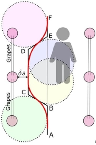
For obstacle avoidance, the robot must first shift in one direction and cross the obstacle, and then resume its position in the center of the lane. Since smooth path generation requires a set of three points, obstacle avoidance requires a set of six points (or two sets each of three points). These points can be generated in real-time for both static and dynamic obstacles. One of the points can be the starting position of the robot itself, i.e., the current position. The other two points need to be generated considering the width of the vineyard lane ($\mathrm{W}$) and the safety threshold (${\delta }_s$). For safety, it is ideal for the robots to navigate the center of the vineyard lane ($x=\frac{\mathrm{W}}{2}$), keeping ample distance from grapes on both the sides. Hence, one of the points is ($x=\frac{\mathrm{W}}{2},\mathrm{y}$). The three points of the first set for the robot to shift in either direction are given as,

$$P=\left\{\mathrm{A}:\left(\frac{\mathrm{W}}{2},\mathrm{y}\right),\mathrm{B}:\left(\frac{\mathrm{W}}{2},\mathrm{y}+{\psi }_1\right),\mathrm{C}:\left(\frac{\mathrm{W}}{\lambda },\mathrm{y}+2{\psi }_2\right)\right\}.$$

(8)

Here, the point $\mathrm{A}=(\frac{\mathrm{W}}{2},\mathrm{y})$ and $\mathrm{B}=(\frac{\mathrm{W}}{2},\mathrm{y}+{\psi }_1)$ are on the center of the lane. Assuming that the robot is shifting towards the left for collision avoidance, the point $\mathrm{C}=(\frac{\mathrm{W}}{\lambda },\mathrm{y}+2{\psi }_2)$ lies on the left side of the corridor. The parameter $\lambda$ controls the distance of the trajectory from the left lane of the vineyard. Considering the width of the robot, we set $\lambda$ to 4, which generates a trajectory at a distance of $\frac{\mathrm{W}}{4}$ from the left vineyard lane. The parameter ${\psi }_1$ determines the starting point of the turn on the current trajectory, while the parameter ${\psi }_2$ controls the turning point after the robot has crossed the obstacle. After that, the robot must maneuver to resume the center of the lane. This requires the generation of the second set of three points which are given as,

$$P^{\prime }=\left\{\mathrm{D}:\left(\frac{\mathrm{W}}{\lambda },{\mathrm{y}}_{\mathrm{t}}\right),\mathrm{E}:\left(\frac{\mathrm{W}}{\lambda },{\mathrm{y}}_{\mathrm{t}}+{\psi }_2\right),\mathrm{F}:\left(\frac{\mathrm{W}}{2},{\mathrm{y}}_{\mathrm{t}}+2{\psi }_2\right)\right\}.$$

(9)

Figure 6b shows the six points $\mathrm{A},\mathrm{B},\mathrm{C},\mathrm{D},\mathrm{E}$ and $\mathrm{F}$. Figure 6b shows the scenario of a vineyard lane with grapes on either side shown by small circles. A person is shown as an obstacle. The smooth trajectory for collision avoidance is shown in red color. It should be noted that a total of four circles needs to be fitted in the trajectory for collision avoidance. The first segment is fitted using points $\mathrm{A},\mathrm{B}$ and $\mathrm{C}$. The other three segments are fitted using points {$\mathrm{B},\mathrm{C},\mathrm{D}$}, {$\mathrm{C},\mathrm{D},\mathrm{E}$}, and {$\mathrm{D},\mathrm{E},\mathrm{F}$}, respectively.

The overall algorithm for obstacle avoidance is given in Figure 7. First, Algorithm 1 is used to detect the pillar positions. Next, the robot centers itself in the center of the lane and stars navigation. If an obstacle is detected, Lidar data are used to estimate its position, whether the obstacle is dynamic or static, and its relative speed if the obstacle is dynamic. Since the robot navigates the center of the lane, it decides the direction of turn (i.e., left or right) to avoid the obstacle. This is typically the opposite direction of the obstacle’s position. Next, for the first maneuver, a set of three points (P) are set and the robot executes the turn on the smooth trajectory. The robot then moves in a straight line keeping a safe distance from the grapes. Once the robot has crossed over the obstacle on the straight path, a set of three new points ($P^{\prime }$) are generated, as given in Figure 7. The robot then executes another smooth turn to come back to the center of the lane. Once this has been performed, the robot continues its navigation through the center of the vineyard’s lane.

Estimating the position of a person is straightforward with a 2D Lidar sensor. The robot has a SLAM (simultaneous localization and mapping) module, which gives the current coordinates of the robot ($x_t^r,y_t^r$) at time t. If ($x_t^p,y_t^p$) are the coordinates of the person, then the distance between the robot and the person is $\sqrt{{(x_t^r-x_t^p)}^2+{(y_t^r-y_t^p)}^2}$. If v is the robot’s velocity and $\theta$ is the heading of the robot, then in time $\Delta t$, the coordinates of the robot are ($x_t^r+\Delta t·v\cos \left(\theta \right),y_t^r+\Delta t·v\sin \left(\theta \right)$). At time $t=t+\Delta t$, the coordinates of the person estimated from the Lidar sensor are ($x_{t+1}^p,y_{t+1}^p$). From the current robot’s and person’s position, distance, and velocity is estimated. Moreover, static and dynamic obstacles are differentiated.

4. Experiment and Results

The algorithm was first evaluated in a simulation environment. The results of simulation are shown in Figure 8. Figure 8a shows the effects of the parameter $\lambda$ on the curvature of the generated trajectories. The robot’s starting position is in the center of the lane at $x=150$. The red circles indicate the detected pillars in the vineyard in the lane. An obstacle was placed at around $x=200,y=180$. Different trajectories were generated with different values of $\lambda =2.5,\lambda =3,\lambda =4,\lambda =6,\lambda =8$, and $\lambda =12$. These trajectories have been marked as $\mathrm{A},\mathrm{B},\mathrm{C},\mathrm{D},\mathrm{E}$, and $\mathrm{F}$, respectively. Similarly, Figure 8b shows the effect of $\psi$ on the generated trajectories.

It can be seen that the different trajectories maintain different safety clearance from the obstacle and the crop. This is shown in Figure 9. The clearance of trajectories marked as $\mathrm{A},\mathrm{B},\mathrm{C},\mathrm{D},\mathrm{E}$ and $\mathrm{F}$ (in Figure 8) from the pillars (and therefore grapes/crop) is shown in Figure 9a. Similarly, the clearance of trajectories marked as $\mathrm{A},\mathrm{B},\mathrm{C},\mathrm{D},\mathrm{E}$ and $\mathrm{F}$ from the obstacle is shown in Figure 9b. It is evident that the trajectory with the largest $\lambda$ value of 12 shown in black color is the closest to the crop. On the other hand, the trajectory with the smallest $\lambda$ value of 2.5 shown in magenta color is the farthest away from the crop. The safety clearance of the trajectories is inversely proportional to the value of $\lambda$. As seen from Figure 8b, the parameter $\psi$ controls how far the curved trajectory extends from the robot while maintaining a constant $\lambda$. Thus, appropriate trajectories that keep a safe distance from the grapes and the obstacles can be generated.

The proposed algorithm was also tested on an actual robot in the vineyard. Figure 10 shows the robot used in the experiment. Robotnik’s Summit-XL robot was used in the experiment. It was equipped with UTM-30LX Lidar, a camera, and control PC with Ubuntu Linux operating system running ROS (Robot Operating System) [51]. The proposed algorithm was developed in Python language on the top of ROS middleware.

Figure 11 shows the straight navigation of the robot by detecting the pillars and traversing the center of the vineyard’s lanes. It can be seen that the robot smoothly traverses the center of the lane without coming close to the crops.

The algorithm was also tested with dynamic obstacles. The timely snapshots of the experiment are shown in Figure 12. In the experiment, the robot initially navigates the center of the vineyard’s lane, as shown in Figure 12a–c. A person approaches the robot walking from the opposite direction, as shown in Figure 12d–i. The algorithm estimated that the person is approaching from the right side of the lane from the point of view of the robot. Hence, a left turn was decided. A smooth trajectory was generated using the proposed algorithm and the robot started executing it, as shown in Figure 12g–j. Once the robot has crossed the person (Figure 12k), the robot then generates a trajectory to resume the center of the lane. This is shown in Figure 12l–o. The robot then resumes navigation in the center of the lane, as shown in Figure 12p–t. The total execution time of pillar detection and smooth trajectory detection was within 70 milliseconds.

It should be noted that there could be scenarios when there are obstacles on both sides of the lane, or lane traversal is not possible. Although this case was not tested in the experiments, the algorithm has a feature that, for such cases, the robot stops its navigation for safety and waits until the obstacles have cleared.

5. Conclusions

In this paper, we proposed an algorithm for autonomous and safe navigation of mobile robots in vineyards. A robust obstacle detection is inherent to mobile robots in vineyards for different applications such as harvesting and monitoring. The algorithm detects the pillars fixed in the vineyards from Lidar data using a symmetric derivative. Compared to image processing-based detection algorithms, the proposed algorithm is not prone to changing the brightness of the environment and can also be used in low light. The robot can navigate the center of the lane from the extracted pillar positions. An algorithm for smooth collision avoidance for static and dynamic obstacles was also proposed. The parameters of the algorithm can be adjusted to keep the robot safe from both the grapes and the obstacles. The proposed algorithm was tested in both simulation and actual environments. In the future, we plan to test the algorithm in more complex scenarios with different applications such as weed detection and harvesting. Using different sensors such as a camera and Lidar sensor for improved pillar and obstacle detection in the presence of tall weeds is also considered as future work.

References

- Japan’s Ministry of Agriculture, Forestry and Fisheries (MAFF). Census of Agriculture in Japan. 2015. Available online: https://www.maff.go.jp/j/wpaper/w_maff/h26/h26_h/trend/part1/chap2/c2_1_03.html (accessed on 1 July 2021).
- Wikipedia. Quasi-Zenith Satellite System. 2021. Available online: https://en.wikipedia.org/wiki/Quasi-Zenith_Satellite_System (accessed on 12 September 2021).
- Japan Aerospace Exploration Agency (JAXA). About Quasi-Zenith Satellite-1 “MICHIBIKI”. 2021. Available online: https://global.jaxa.jp/projects/sat/qzss/ (accessed on 12 September 2021).
- Ravankar, A.; Ravankar, A.A.; Kobayashi, Y.; Jixin, L.; Emaru, T.; Hoshino, Y. A novel vision based adaptive transmission power control algorithm for energy efficiency in wireless sensor networks employing mobile robots. In Proceedings of the 2015 Seventh International Conference on Ubiquitous and Future Networks, Sapporo, Japan, 7–10 July 2015; pp. 300–305. [Google Scholar] [CrossRef]
- Ravankar, A.; Ravankar, A.A.; Hoshino, Y.; Emaru, T.; Kobayashi, Y. On a Hopping-points SVD and Hough Transform Based Line Detection Algorithm for Robot Localization and Mapping. Int. J. Adv. Robot. Syst. 2016, 13, 98. [Google Scholar] [CrossRef] [Green Version]
- Ravankar, A.A.; Hoshino, Y.; Ravankar, A.; Jixin, L.; Emaru, T.; Kobayashi, Y. Algorithms and a framework for indoor robot mapping in a noisy environment using clustering in spatial and Hough domains. Int. J. Adv. Robot. Syst. 2015, 12, 27. [Google Scholar] [CrossRef] [Green Version]
- Vinbot. 2020. Available online: http://vinbot.eu/ (accessed on 11 July 2021).
- Ly, O.; Gimbert, H.; Passault, G.; Baron, G. A Fully Autonomous Robot for Putting Posts for Trellising Vineyard with Centimetric Accuracy. In Proceedings of the 2015 IEEE International Conference on Autonomous Robot Systems and Competitions, Vila Real, Portugal, 8–10 April 2015; pp. 44–49. [Google Scholar] [CrossRef]
- Igawa, H.; Tanaka, T.; Kaneko, S.; Tada, T.; Suzuki, S. Visual and tactual recognition of trunk of grape for weeding robot in vineyards. In Proceedings of the 2009 35th Annual Conference of IEEE Industrial Electronics, Porto, Portugal, 3–5 November 2009; pp. 4274–4279. [Google Scholar] [CrossRef]
- Thayer, T.C.; Vougioukas, S.; Goldberg, K.; Carpin, S. Multi-Robot Routing Algorithms for Robots Operating in Vineyards. In Proceedings of the 2018 IEEE 14th International Conference on Automation Science and Engineering (CASE), Munich, Germany, 20–24 August 2018; pp. 14–21. [Google Scholar] [CrossRef]
- Gao, M.; Lu, T. Image Processing and Analysis for Autonomous Grapevine Pruning. In Proceedings of the 2006 International Conference on Mechatronics and Automation, Luoyang, China, 25–28 June 2006; pp. 922–927. [Google Scholar] [CrossRef] [Green Version]
- Riggio, G.; Fantuzzi, C.; Secchi, C. A Low-Cost Navigation Strategy for Yield Estimation in Vineyards. In Proceedings of the 2018 IEEE International Conference on Robotics and Automation (ICRA), Brisbane, QLD, Australia, 21–25 May 2018; pp. 2200–2205. [Google Scholar] [CrossRef]
- Nuske, S.; Achar, S.; Bates, T.; Narasimhan, S.; Singh, S. Yield estimation in vineyards by visual grape detection. In Proceedings of the 2011 IEEE/RSJ International Conference on Intelligent Robots and Systems, San Francisco, CA, USA, 25–30 September 2011; pp. 2352–2358. [Google Scholar] [CrossRef] [Green Version]
- Thayer, T.C.; Vougioukas, S.; Goldberg, K.; Carpin, S. Routing Algorithms for Robot Assisted Precision Irrigation. In Proceedings of the 2018 IEEE International Conference on Robotics and Automation (ICRA), Brisbane, QLD, Australia, 21–25 May 2018; pp. 2221–2228. [Google Scholar] [CrossRef]
- Contente, O.M.D.S.; Lau, J.N.P.N.; Morgado, J.F.M.; Santos, R.M.P.M.D. Vineyard Skeletonization for Autonomous Robot Navigation. In Proceedings of the 2015 IEEE International Conference on Autonomous Robot Systems and Competitions, Vila Real, Portugal, 8–10 April 2015; pp. 50–55. [Google Scholar] [CrossRef]
- Gay-Fernández, J.A.; Cuiñas, I. Deployment of a wireless sensor network in a vineyard. In Proceedings of the International Conference on Wireless Information Networks and Systems, Seville, Spain, 18–21 July 2011; pp. 35–40. [Google Scholar]
- Galmes, S. Lifetime Issues in Wireless Sensor Networks for Vineyard Monitoring. In Proceedings of the 2006 IEEE International Conference on Mobile Ad Hoc and Sensor Systems, Vancouver, BC, Canada, 9–12 October 2006; pp. 542–545. [Google Scholar]
- Wigneron, J.; Dayan, S.; Kruszewski, A.; Aluome, C.; AI-Yaari, M.G.A.; Fan, L.; Guven, S.; Chipeaux, C.; Moisy, C.; Guyon, D.; et al. The Aqui Network: Soil Moisture Sites in the “Les Landes” Forest and Graves Vineyards (Bordeaux Aquitaine Region, France). In Proceedings of the IGARSS 2018—2018 IEEE International Geoscience and Remote Sensing Symposium, Valencia, Spain, 22–27 July 2018; pp. 3739–3742. [Google Scholar]
- Ye, F.; Qi, W. Design of wireless sensor node for drought monitoring in vineyards. In Proceedings of the International Conference on Advanced Infocomm Technology 2011 (ICAIT 2011), Wuhan, China, 11–14 July 2011. [Google Scholar] [CrossRef]
- Sánchez, N.; Martínez-Fernández, J.; Aparicio, J.; Herrero-Jiménez, C.M. Field radiometry for vineyard status monitoring under Mediterranean conditions. In Proceedings of the 2014 IEEE Geoscience and Remote Sensing Symposium, Quebec City, QC, Canada, 13–18 July 2014; pp. 2094–2097. [Google Scholar]
- Pérez-Expósito, J.P.; Fernández-Caramés, T.M.; Fraga-Lamas, P.; Castedo, L. An IoT Monitoring System for Precision Viticulture. In Proceedings of the 2017 IEEE International Conference on Internet of Things (iThings) and IEEE Green Computing and Communications (GreenCom) and IEEE Cyber, Physical and Social Computing (CPSCom) and IEEE Smart Data (SmartData), Exeter, UK, 21–23 June 2017; pp. 662–669. [Google Scholar]
- Medela, A.; Cendón, B.; González, L.; Crespo, R.; Nevares, I. IoT multiplatform networking to monitor and control wineries and vineyards. In Proceedings of the 2013 Future Network Mobile Summit, Lisboa, Portugal, 3–5 July 2013; pp. 1–10. [Google Scholar]
- Mouakher, A.; Belkaroui, R.; Bertaux, A.; Labbani, O.; Hugol-Gential, C.; Nicolle, C. An Ontology-Based Monitoring System in Vineyards of the Burgundy Region. In Proceedings of the 2019 IEEE 28th International Conference on Enabling Technologies: Infrastructure for Collaborative Enterprises (WETICE), Napoli, Italy, 12–14 June 2019; pp. 307–312. [Google Scholar]
- Ahumada-García, R.; Poblete-Echeverría, C.; Besoain, F.; Reyes-Suarez, J. Inference of foliar temperature profile of a vineyard using integrated sensors into a motorized vehicle. In Proceedings of the 2016 IEEE International Conference on Automatica (ICA-ACCA), Curico, Chile, 19–21 October 2016; pp. 1–6. [Google Scholar]
- Lloret, J.; Bosch, I.; Sendra, S.; Serrano, A. A Wireless Sensor Network for Vineyard Monitoring That Uses Image Processing. Sensors 2011, 11, 6165–6196. [Google Scholar] [CrossRef] [PubMed] [Green Version]
- de Santos, F.B.N.; Sobreira, H.M.P.; Campos, D.F.B.; de Santos, R.M.P.M.; Moreira, A.P.G.M.; Contente, O.M.S. Towards a Reliable Monitoring Robot for Mountain Vineyards. In Proceedings of the 2015 IEEE International Conference on Autonomous Robot Systems and Competitions, Vila Real, Portugal, 8–10 April 2015; pp. 37–43. [Google Scholar]
- Roure, F.; Bascetta, L.; Soler, M.; Matteucci, M.; Faconti, D.; Gonzalez, J.P.; Serrano, D. Lessons Learned in Vineyard Monitoring and Protection from a Ground Autonomous Vehicle. In Advances in Robotics Research: From Lab to Market: ECHORD++: Robotic Science Supporting Innovation; Grau, A., Morel, Y., Puig-Pey, A., Cecchi, F., Eds.; Springer International Publishing: Cham, Switzerland, 2020; pp. 81–105. [Google Scholar] [CrossRef]
- Ravankar, A.; Ravankar, A.A.; Watanabe, M.; Hoshino, Y.; Rawankar, A. Development of a Low-Cost Semantic Monitoring System for Vineyards Using Autonomous Robots. Agriculture 2020, 10, 182. [Google Scholar] [CrossRef]
- Valencia, D.; Kim, D. Quadrotor Obstacle Detection and Avoidance System Using a Monocular Camera. In Proceedings of the 2018 3rd Asia-Pacific Conference on Intelligent Robot Systems (ACIRS), Singapore, 21–23 July 2018; pp. 78–81. [Google Scholar] [CrossRef]
- Touzene, N.B.; Larabi, S. Obstacle Detection from Uncalibrated Cameras. In Proceedings of the 2008 Panhellenic Conference on Informatics, Samos, Greece, 28–30 August 2008; pp. 152–156. [Google Scholar] [CrossRef]
- Jung, J.I.; Ho, Y.S. Depth map estimation from single-view image using object classification based on Bayesian learning. In Proceedings of the 2010 3DTV-Conference: The True Vision—Capture, Transmission and Display of 3D Video, Tampere, Finland, 7–9 June 2010; pp. 1–4. [Google Scholar] [CrossRef]
- Hambarde, P.; Dudhane, A.; Murala, S. Single Image Depth Estimation Using Deep Adversarial Training. In Proceedings of the 2019 IEEE International Conference on Image Processing (ICIP), Taipei, Taiwan, 22–25 September 2019; pp. 989–993. [Google Scholar] [CrossRef]
- Kuo, T.Y.; Hsieh, C.H.; Lo, Y.C. Depth map estimation from a single video sequence. In Proceedings of the 2013 IEEE International Symposium on Consumer Electronics (ISCE), Hsinchu, Taiwan, 3–6 June 2013; pp. 103–104. [Google Scholar] [CrossRef]
- Ravankar, A.; Ravankar, A.A.; Kobayashi, Y.; Emaru, T. SHP: Smooth Hypocycloidal Paths with Collision-Free and Decoupled Multi-Robot Path Planning. Int. J. Adv. Robot. Syst. 2016, 13, 133. [Google Scholar] [CrossRef] [Green Version]
- Durham, J.W.; Bullo, F. Smooth Nearness-Diagram Navigation. In Proceedings of the 2008 IEEE/RSJ International Conference on Intelligent Robots and Systems, Nice, France, 22–26 September 2008; pp. 690–695. [Google Scholar] [CrossRef] [Green Version]
- Minguez, J.; Montano, L.; Simeon, T.; Alami, R. Global nearness diagram navigation (GND). In Proceedings of the 2001 ICRA, IEEE International Conference on Robotics and Automation (Cat. No.01CH37164), Seoul, Korea, 21–26 May 2001; Volume 1, pp. 33–39. [Google Scholar] [CrossRef]
- Song, B.; Tian, G.; Zhou, F. A comparison study on path smoothing algorithms for laser robot navigated mobile robot path planning in intelligent space. J. Inf. Comput. Sci. 2010, 7, 2943–2950. [Google Scholar]
- Ravankar, A.; Ravankar, A.; Kobayashi, Y.; Hoshino, Y.; Peng, C.C. Path Smoothing Techniques in Robot Navigation: State-of-the-Art, Current and Future Challenges. Sensors 2018, 18, 3170. [Google Scholar] [CrossRef] [PubMed] [Green Version]
- Delling, D.; Sanders, P.; Schultes, D.; Wagner, D. Engineering Route Planning Algorithms. In Algorithmics of Large and Complex Networks; Lecture Notes in Computer Science; Lerner, J., Wagner, D., Zweig, K., Eds.; Springer: Berlin/Heidelberg, Germany, 2009; Volume 5515, pp. 117–139. [Google Scholar] [CrossRef] [Green Version]
- LaValle, S.M. Planning Algorithms; Cambridge University Press: Cambridge, UK, 2006; Available online: http://planning.cs.uiuc.edu/ (accessed on 11 February 2016).
- Latombe, J.C. Robot Motion Planning; Kluwer Academic Publishers: Norwell, MA, USA, 1991. [Google Scholar]
- Ravankar, A.; Ravankar, A.A.; Rawankar, A.; Hoshino, Y.; Kobayashi, Y. ITC: Infused Tangential Curves for Smooth 2D and 3D Navigation of Mobile Robots. Sensors 2019, 19, 4384. [Google Scholar] [CrossRef] [PubMed] [Green Version]
- Dijkstra, E.W. A Note on Two Problems in Connexion with Graphs. Numer. Math. 1959, 1, 269–271. [Google Scholar] [CrossRef] [Green Version]
- Hart, P.; Nilsson, N.; Raphael, B. A Formal Basis for the Heuristic Determination of Minimum Cost Paths. IEEE Trans. Syst. Sci. Cybern. 1968, 4, 100–107. [Google Scholar] [CrossRef]
- Stentz, A. The Focussed D* Algorithm for Real-Time Replanning. In Proceedings of the International Joint Conference on Artificial Intelligence, Montreal, QC, Canada, 20–25 August 1995; pp. 1652–1659. [Google Scholar]
- Stentz, A.; Mellon, I.C. Optimal and Efficient Path Planning for Unknown and Dynamic Environments. Int. J. Robot. Autom. 1993, 10, 89–100. [Google Scholar]
- Kavraki, L.; Svestka, P.; Latombe, J.C.; Overmars, M. Probabilistic roadmaps for path planning in high-dimensional configuration spaces. IEEE Trans. Robot. Autom. 1996, 12, 566–580. [Google Scholar] [CrossRef] [Green Version]
- Lavalle, S.M. Rapidly-Exploring Random Trees: A New Tool for Path Planning; Technical Report 98-11; Computer Science Department, Iowa State University: Ames, IA, USA, 1998. [Google Scholar]
- LaValle, S.M.; Kuffner, J.J. Randomized Kinodynamic Planning. Int. J. Robot. Res. 2001, 20, 378–400. [Google Scholar] [CrossRef]
- Lavalle, S.M.; Kuffner, J.J., Jr. Rapidly-Exploring Random Trees: Progress and Prospects. Algorithmic Comput. Robot. New Dir. 2000, 5, 293–308. [Google Scholar]
- Quigley, M.; Conley, K.; Gerkey, B.P.; Faust, J.; Foote, T.; Leibs, J.; Wheeler, R.; Ng, A.Y. ROS: An open-source Robot Operating System. ICRA Workshop Open Source Softw. 2009, 3, 5. [Google Scholar]
Figure 1.
(a) Population and average age of farmers in Japan. Data from Japan’s Ministry of Agriculture, Forestry and Fisheries (MAFF) [1]. (b) Census of agriculture in Japan [1].
Figure 2.
Standing of proposed research (yellow block) in Vineyard robots. Path planning and obstacle avoidance is a core module of mobile robots that supports top-level applications such as harvesting, weed removal, monitoring, and estimation.
Figure 3.
Three different scenarios of pillar detection in a vineyard. The Lidar data and its symmetric derivate are shown on the right. (a) Single pillar case. (b) Two pillars on either side. (c) Occluded pillars. (g–i) show the actual pictures of the three scenarios in a vineyard.
Figure 4.
Grape stem, weed, and pillar in a vineyard. The Lidar sensor is setup at a height greater than that of the weeds. Hence, noise from weeds does not affect the accuracy of pillar detection.
Figure 5.
Simulation result of pillar detection. Lidar data are shown in blue, whereas its symmetric derivative is shown in orange color. The detected pillar is shown in red circle between the rising and falling edges of the symmetric derivative.
Figure 6.
Smooth obstacle avoidance. (a) Generation of smooth trajectories at turns using segments of circular arcs. (b) Obstacle avoidance using smooth trajectories shown in red color keeping a safe distance from the crop.
Figure 7.
Flowchart of obstacle avoidance algorithm.
Figure 8.
Effects of parameters and on trajectories generated. (a) Different trajectories generated with different values. (b) Trajectories generated with different values.
Figure 9.
Safety distance of robot from the crop and the obstacle in case of simulation in Figure 8a. (a) Distances of different trajectories from the crop. (b) Distances of different trajectories from the obstacle.
Figure 10.
Robotnik’s Summit-XL robot used in the experiment with UTM-30LX Lidar, camera, and control computer.
Figure 11.
(a–h) shows the successive snapshots of autonomous robot navigation in the center of vineyard’s lane using the proposed algorithm. The video of the experiment is provided in the supplementary section.
Figure 12.
(a–t) Timely snapshots of dynamic obstacle (incoming person) avoidance in the vineyard using the proposed algorithm. The video of the experiment is provided in the supplementary section.
Publisher’s Note: MDPI stays neutral with regard to jurisdictional claims in published maps and institutional affiliations. |
© 2021 by the authors. Licensee MDPI, Basel, Switzerland. This article is an open access article distributed under the terms and conditions of the Creative Commons Attribution (CC BY) license (https://creativecommons.org/licenses/by/4.0/).
Share and Cite
MDPI and ACS Style
Ravankar, A.; Ravankar, A.A.; Rawankar, A.; Hoshino, Y. Autonomous and Safe Navigation of Mobile Robots in Vineyard with Smooth Collision Avoidance. Agriculture 2021, 11, 954. https://doi.org/10.3390/agriculture11100954
AMA Style
Ravankar A, Ravankar AA, Rawankar A, Hoshino Y. Autonomous and Safe Navigation of Mobile Robots in Vineyard with Smooth Collision Avoidance. Agriculture. 2021; 11(10):954. https://doi.org/10.3390/agriculture11100954
Chicago/Turabian StyleRavankar, Abhijeet, Ankit A. Ravankar, Arpit Rawankar, and Yohei Hoshino. 2021. "Autonomous and Safe Navigation of Mobile Robots in Vineyard with Smooth Collision Avoidance" Agriculture 11, no. 10: 954. https://doi.org/10.3390/agriculture11100954
Note that from the first issue of 2016, this journal uses article numbers instead of page numbers. See further details here.