Using SPOT-7 for Nitrogen Fertilizer Management in Oil Palm
by
 ,
,
Mohammad Yadegari
1, 
Redmond R. Shamshiri
2,* ,
,
Abdul Rashid Mohamed Shariff
1,
Siva K. Balasundram
3 and
Benjamin Mahns
2 1
Department of Biological and Agricultural Engineering, Faculty of Engineering, Universiti Putra Malaysia, Serdang 43400, Malaysia
2
Leibniz Institute for Agricultural Engineering and Bioeconomy, Max-Eyth-Allee 100, 14469 Potsdam-Bornim, Germany
3
Department of Agriculture Technology, Faculty of Agriculture, Universiti Putra Malaysia, Serdang 43400, Malaysia
*
Author to whom correspondence should be addressed.
Agriculture 2020, 10(4), 133; https://doi.org/10.3390/agriculture10040133
Submission received: 23 January 2020
/
Revised: 2 April 2020
/
Accepted: 9 April 2020
/
Published: 17 April 2020
(This article belongs to the Section Agricultural Systems and Management)
Abstract
:Environmental concerns are growing about excessive applying nitrogen (N) fertilizers, especially in oil palm. Some conventional methods which are used to assess the amount of nutrient in oil palm are time-consuming, expensive, and involve frond destruction. Remote sensing as a non-destructive, affordable, and efficient method is widely used to detect the concentration of chlorophyll (Chl) from canopy plants using several vegetation indices (VIs) because there is an influential relation between the concentration of N in the leaves and canopy Chl content. The objectives of this research are to (i) evaluate and compare the performance of various vegetation indices (VIs) for measuring N status in oil palm canopy using SPOT-7 imagery (AIRBUS Defence & Space, Ottobrunn, Germany) to (ii) develop a regression formula that can predict the N content using satellite data to (iii) assess the regression formula performance on testing datasets by testing the coefficient of determination between the predicted and measured N contents. SPOT-7 was acquired in a 6-ha oil palm planted area in Pahang, Malaysia. To predict N content, 28 VIs based on the spectral range of SPOT-7 satellite images were evaluated. Several regression models were applied to determine the highest coefficient of determination between VIs and actual N content from leaf sampling. The modified soil-adjusted vegetation index (MSAVI) generated the highest coefficient of determination (R2 = 0.93). MTVI1 and triangular VI had the highest second and third coefficient of determination with N content (R2 = 0.926 and 0.923, respectively). The classification accuracy assessment of the developed model was evaluated using several statistical parameters such as the independent t-test, and p-value. The accuracy assessment of the developed model was more than 77%.
1. Introduction
Oil palm (Elaeis guineensis) is a species of palm that provides one of the leading vegetable oils produced globally, accounting for one quarter of global consumption and approximately 60% of international trade in vegetable oils [1]. Malaysia and Indonesia are the main key players in the palm oil sector, and these two countries together account for about 90% of the global palm oil export. The oil palm industry is considered a very profitable one in Malaysia; hence, the plantation of oil palm has increased significantly over the years [2]. Over the last decade, specifically from 2005 to 2015, the oil palm planted area has increased by 42% in the country. Currently, Malaysia has the second largest area under oil palm cultivation after Indonesia. The export trends of oil palm by-products also increased by 9% from 2008 to 2016 in Malaysia [3]. However, the sector is likely to have its profitability reduced due to the decline of world prices, high-cost conventional farming practices, and loss of production due to nutrition deficiencies, pests, and disease. The Malaysian oil palm industry specifically suffers from the high costs of labor and low yields due to poor fertilizer management, to the extent that the country’s place is being threatened by Indonesia in the profitable oil palm market [2]. Appropriate pest and fertilizer management can increase the production of oil palm by managing the pests and diseases as well as solving the nutrition problems of plants. Besides, an efficient management solution can reduce labor efforts and costs; hence, increasing the profitability of the plantations [4].
One of the most critical deficiencies that influence the production of any crop, and in particular, oil palm, is nitrogen (N). In plant growth, physiology, and carbohydrate content terms, N is the most critical nutrient element [5,6]. In an oil palm plantation, the common practice to achieve the best yield quantitatively is to add N via fertilizers. In Malaysia, 46% to 85% of field costs go into the purchase of the fertilizers alone [7,8,9]. According to Figure 1, Malaysia is ranked the world’s second highest fertilizer consumer with 2063.9 Kg fertilizers per ha in 2014 after Qatar [10], while the two neighbors of Malaysia, Indonesia and Thailand, only used 211.8 and 152.3 kg per ha, respectively, which are 89% and 92% less than Malaysia. Compared to Australia, Malaysia’s consumption of fertilizer is 3708.98% higher, as well [11].
Besides, the excessive fertilizer use can cause several environmental and ecological problems, such as air pollution, soil acidification and degradation, water eutrophication, crop yield reduction, and, finally, decreasing the sustainability of the agricultural practices [12]. Specifically, there is a severe concern about the excess use of N fertilizers in oil palm plantations because of N losses and N leaching. For instance, the amount of N fertilizers commonly applied to produce 1 ton of fresh fruit branches (FFB) generates around 50% of greenhouse gasses (GHG) [8,13]. According to the several surveys, leaf sampling and analysis is the most common method to assess the nutrient status in oil palm leaf [14,15]. In 2013, the total costs for annual leaf sampling and analysis in Malaysia were estimated at around MYR 2,564,346 (Equivalent to USD 600,000), with 5.2 million ha area under oil palm cultivation [16]. It is worthwhile to note that the area under oil palm cultivation increased to 5.8 million ha in 2017; hence, the total cost of oil palm production accounting for labor costs, leaf sampling and analysis has also risen.
Satellite imagery, as one of the remote sensing tools, can be used effectively to identify nutrient status in oil palm trees [17]. Information from these images helps for early identification of diseases, such as Ganoderma and Armillaria trunk rot [4,17], within a field remotely before they can be visually identified. This information allows an accurate prediction of nitrogen fertilizer needs at each point in the field at a lower cost. As a result, the crop yield can be increased. This approach would also reduce surplus fertilizer in the crop production system without reducing crop yield, which would, in return, reduce N losses to surface and ground waters.
Further, a remotely sensed fertilizer management system based on satellite imageries can reduce the labor costs associated with leaf sampling, and laboratories related costs [18]. Research findings have shown that ground-based remote sensing techniques, compared to aerial imaging, have a lower efficiency due to sample size limitations, and hence lower accuracy to predict the amount of the nutrient in oil palm is rather weak [19]. Overall, Malaysia can benefit from the advantages that remote sensing techniques offer to narrow down the gap in the yield, sale, and profit margins between its production amount and the top country in the oil palm sector, Indonesia.
One of the useful tools to estimate biophysical parameters of plants using satellite sensors is spectral remote sensing [20]. Many studies have reported that there is a good coefficient of determination between the N concentration in the canopy and the amount of chlorophyll obtained from spectral vegetation indices [21,22,23]. Satellite sensors with high spatial resolution, usually 10 m or lower, have recently been used for assessing the nutrient status, especially N, in different crops. Zhang et al. [24] showed that the status of N could be detected using IKONOS Satelite (Lockheed Corporation, Calabasas, CA, USA) data in rice. Wu [25] evaluated the reliability of QuickBird to detect the biophysical and biochemical characteristics of potato. The standard spectral VIs were examined to detect the best VI for predicting the amount of N in potato. The results showed that MSAVI had the highest coefficient of determination between the satellite data and the ground data. In another research, Shou et al. [26] used the QuichBird satellite, which is a high-resolution sensor (below 10 m), to evaluate the status of N in winter wheat. This study illustrated that all broadband indices from satellite images correlated well with the amount of N concentration from the canopy. They also showed that there is a high potential to use satellite imagery with a high spatial resolution for N status diagnosis. Eitel et al. [27] used RapidEye to predict N status of spring wheat and found a high correlation (R-square > 0.9) between image data and chlorophyll meter values. In addition, the study showed that the ratio of MCARI/MTVI2 (the ratio of the modii ed chlorophyll absorption ratio index to the second modii ed triangular vegetation index) obtained was the best VI which can predict the N concentration of leaves. Schelling [28] studied different single, combined, and distance VIs to find a relationship between RapidEye satellite imagery and soil–plant analysis development (SPAD) that can measure the amount of N in the wheat leaf. The study reported that NDRE/NDVI (the normalized difference red edge index to normalized difference vegetation index), which is a combined VI with = 0.77, had the highest coefficient of determination among the rest of VIs. Nikrooz et al. [29] predicted corn canopy N content using satellite imagery from Aster. They generated an N fertilization map using a spectral angle mapper (SAM) classifier. They also confirmed that MTVI2 had the highest coefficient of determination (= 0.87), and it was the best predictor for N content in corn canopy. O’Connell et al. [30] used RapidEye to estimate the status of N in almond to reduce the cost of sampling size, and to account for effects of vegetation cover. The study proved that NDVI and CCCI (canopy chlorophyll content index) are two useful VIs for deriving multi-temporal and multi-locational crop data. In another try, Omer et al. [31] used WorldView-2 (WV-2) imagery to monitor the N concentration and the amount of C in forest trees. They also compared the difference between support vector machines (SVM) and artificial neural network (ANN). In this study, they found that the regressions achieved from SVM were more accurate than ANN for estimating the concentration of forest foliar N and C. A summary of the reviewed research findings is provided in Table 1.
In the present study, the goals are to evaluate and compare the performance of various vegetation indices (VIs) for measuring N status in oil palm canopy using SPOT-7 imagery and to develop a regression formula that can predict the N content using satellite data. Moreover, the performance of the regression formula would be assessed by testing the coefficient of determination between the predicted and measured N contents on testing datasets.
2. Materials and Methods
2.1. Study Area
The experiment was carried out in collaboration with FELDA (Federal Land Development Authority) Plantation Sdn. Bhd, a company that has played a significant role in the development of the oil palm industry in Malaysia. Figure 2 represents the location map of the study area in this research in Pahang.
The study was conducted a 6-ha field with 7-years old healthy oil palms (Elaeis guineensis Jacq) in Pahang, Malaysia. The study area was divided into three plots: A, B, and C, according to a randomized complete block design (RCBD). The RCBD is the standard design for agricultural experiments in where similar experimental units are grouped into blocks or replicates. Most of the agricultural experiments were carried out on Plot A, and it was in good agronomic practice, while there were no agricultural practices for Plot C. Table 2a,b represents essential information and differences between the plots, respectively. Specifically, three different types of legumes as crop cover, namely, Mucuna bracteata (Mb), Centrosema Molle (CM), and Pueraria Javanica (PJ), were used in Plots A and B.
In terms of applying fertilizers, FELDA has applied the same types and the same amounts of fertilizers for this area. Table 3 illustrates the different types of fertilizers used, the application date, and the amount of fertilizers in kg per tree that had been used in 18 plots equally between 2015 to 2016. Compound fertilizers (CPD) such as 15-15-15 and NK Mix (20-10) were two conventional inorganic fertilizers that were used by FELDA company in the study area.
2.2. Data Collection
In this study, two different types of data were used. First, the ground data was collected after leaf sampling and leaf analysis, and then, image processing was carried out to collect satellite data. Leaf sampling and analysis is the main part of a procedure adapted by farmers to measure the status of leaf nutrient and the fertilizer need. The leaf sampling was carried out by trained workers from FELDA company from 22–31 March 2016. The study area was divided into 18 plots, with each plot having length and width of 450 and 74.5 m, respectively, as shown in Figure 3. From each plot, 24 palms were selected randomly for sampling the leaves. The justification behind the number of palms was based on the significant differences between leaf samples of the palms (status of leaf nutrient), as suggested by agricultural experts and farmers.
Figure 4 represents the position of the trees selected by workers in orange points. The coordinates of the selected trees were collected using GPS Map 76cSX (Garmin Ltd, Olathe, Kansas, USA) with an accuracy of 1 m. Since the accuracy of GPS was higher than the spatial resolution of each pixel in the image, the application of this type of GPS is reasonable in this research [29]. Frond 17 (F17) has been the primary choice for nutrient assessment as it is the center front of the tree, and its nutrients status can represent the nutrition status of the tree very well [7,14,32]. As a result, in this research, only one F17 was taken from each tree as the sample for nutrient measurements. The sampled leaflets from each plot were then combined according to the usual leaf sampling of the region. Multispectral satellite images from the SPOT-7, for a sunny and cloudless day on the study area, was acquired from Airbus Defense and Space on 29 March 2016. Details are given in Table 4.
2.3. Pre-Processing
Geometric correction and radiometric calibration are two pre-steps of satellite imageries processing. The acquired image was geometrically corrected in ArcMap 10.3 software using a 1:800 scale at the WGS84/UTM Zone 48N projection system with the RMSE of less than 0.2 pixels. Besides, the nearest neighbor method was used as the resampling method. In radiometric correction, the data should be changed from digital numbers (DN’s) to top of atmosphere (TOA) radiance. Although satellite data are analyzed in DNs, they are not suitable to be used in VI studies. It is necessary to convert DNs into radiance first [33,34,35,36,37,38]. In this study, the image was converted from DNs into TOA radiance (physical unit) using Envi5.3, and pre-FLAASH was applied to the image to prepare it for atmospheric correction. The below equation is used to carry out radiometric calibration in SPOT-7, where (p) is the radiance in units of W/ (m2 * sr * µm), and is the digital count of a pixel:
As a critical preprocessing step toward analysis of different VIs, atmospherical correction, including cloud masking of satellite images, was carried according to the procedure described by [39]. The FLAASH atmospheric correction model based on MODTRAN radiative transfer code in Envi5.3 software was used in this study. After using FLAASH atmospheric correction, it is critical to exclude unnecessary surface reflectance pixels such as clouds before subsetting data and applying different VIs on the image [40]. After subsetting the study area, 28 SVIs were calculated in Evvi5.3 software based on spectral features of SPOT-7, using band math and band ratio to predict the canopy leaf N in the oil palm (Table 5). These VIs have been proposed to assess the concentration of N in different canopy plants as well. After applying all 28 VIs, they were transferred into ArcMap 10.3 for extracting the VIs values. Table 5 represents suitable Vis, which can be calculated with SPOT-7 to detect the percentage of chlorophyll in the leaves.
2.4. Statistical Analysis
The statistical analysis was conducted using IBM SPSS 24 software. The polynomial regression model is an approximation method commonly used to find a relationship between dependent variables (DV) and independent variables (IV) with uncertain relationships. In this study, different regression models such as logarithmic, quadratic, compound, power, S, growth, and exponential and linear were investigated to determine the highest relation between VIs and agronomic measurements. In these regression models, the ground data were considered as the dependent variable (DV) and VIs as the independent variable (IV). In this research, the first three replications of the study area, which included nine plots, were considered to investigate the feasibility of different regressions models. The overall performances of the established relationships were analyzed by comparing and the root mean square error (RMSE). The higher the and the lower the RMSE, the higher the precision and the accuracy of the model for predicting plant N status indicators. In the end, the best regression model was applied for the second part of the field to check the accuracy of the results using the independent t-test.
The satellite analysis result starts with radiometric calibration after geometrically correcting the image. The aim of this step is to convert DNs into TOA radiance. Envi software gives the option in this step to users who want to apply pre-require features of FLAASH atmospheric correction. In this research, the software was used to apply the corrections. The SPOT- 7 images in this research were 12 bit, which is equal to 4095 DN. In the end, using region of interest (ROI), the study area was subsetted and the image of the study area was used for applying different VI formulas using the band math option in Envi 5.3. Also, using ArcMap 10.3 software, the pixel values for the selected plants in the leaf sampling method were collected for different VI images. For a continued process, the IBM SPSS Software was used to find the relationship between the percentage of N from ground data, and the data come from different Vis, which present the percentage of chlorophyll (N). Polynomial regression (PR) is one of the most approximation methods that is used to find the relationship between DV and IV. This study, using IBM SPSS 24, tries to find a significant relationship between VIs as X-variables or IVs and leaf nitrogen contents as Y-variables or DVs. To examine the relationship between DV and IV, different regression models such as logarithmic, quadratic, compound, power, S, growth, exponential, and linear were tested [29,65,66].
3. Results and Discussion
Leaf analysis plays an essential role in evaluating the amount of nutrients in the leaves. This method is used to check the status of nutrients in the leaves. In other words, it is used to find any imbalanced interactions or antagonisms and to check whether the amount of fertilizers applied is suitable for the plants or not [67]. Table 6 represents the results of leaves sampling from the laboratory analysis using the Kjeldahl method [68].
According to Table 7, if the concentration of N in the leaves is less than 2.3%, it shows the plots have a deficiency, and if the percentage is more than 3%, it illustrates the surplus or excess of N in the plants. This table shows that the best and optimum amount of N% in the leaf, which is between 2.4% to 2.8%. Comparing these two tables, it shows that most of the plots in the study area had N surplus (11 out of 18), and the rest are in marginal condition.
The datasets in this study are divided 50%–50% for calibration and validation of the fitted models, respectively. First of all, using the first 9 plots of the study area, the best regression model was chosen with the highest R-squared and the lowest RMSE. According to the results and comparing between different VIs, it shows that MSAVI with 0.93 R-squared had a higher one. MTVI, triangular VI, and MCARI1 with 0.926, 0.923, 0.922 occupied second to fourth places, respectively, and among the models, quadratic was the fittest model (Figure 5).
Table 8 represents R, R-squares, adjusted R, and standard error of the estimate for MSAVI with 8 different models. In addition, in Figure 6, the curve-fit illustrates how the different regression models are close to the dependent and independent variables.
According to Figure 5, the MSAVI had the best fit with the leaves sampling data. Also, with comparing different regression models, it was shown that the quadratic method had the fittest curve between other regression methods for DVs and IVs. As a result, this VI was used to develop a quadratic regression model to predict the percentage of N for the second part of the study area.
According to Table 9, there is a high significant relationship between MSAVI and actual N from the field because the p-value or Sig is close to 0. Consequently, the model of predicted N developed in this study is presented in Equation (2). Table 10 shows the predicted N by using the above model.
Before performing an accuracy assessment of the predicted results, it needs to be shown that there is a relationship between predicted N and the actual amount of N. Independent t-test is one of the most common methods that are used to investigate the relationship between two sets of data. The variables used in this test are known as dependent variables (test variable) and independent variables (grouping variable). In this test, IVs should be categorical and include precisely two groups, which are represented in one column. Group 1 is defined for actual N and Group 2 is defined for predicted N. The independent sample t-test requires the assumption of homogeneity of variance, which is called Levene’s test. In this research, the null and alternative hypothesis is expressed as Ho = there is a strong relationship between N predicted, and actual N versus Ha = there is no relationship between N predicted and actual N. This implies that if we accept the null hypothesis of Levene’s test, it suggests that the variances of the two groups are equal, which means that the homogeneity of variances assumption is not violated. SPSS Statistics generated two main tables of output for the independent t-test. Table 11, which is called the group statistic table, provides descriptive statistics for the two groups that were compared, including the mean and standard deviation. Table 4, which is called an independent sample test table, provides the actual results from the independent t-test. According to the results in Table 12, the p-value was much higher than 0.05; hence, the null hypothesis was accepted, which means there was a strong relationship between the percentage of actual N and predicted N.
After representing the relationship between the percentage of actual N and predicted N using the independent t-test, the accuracy assessment was conducted. According to Table 7, N-values < 2.3 are considered a deficiency; N-values between 2.3 to 2.4 are considered marginal level, which can be changed to a deficiency; N-values between 2.4 to 2.8 are considered optimal, and most of the agricultural practices plan to get this level; N values between 2.8 to 3 are second marginal, close to excess; N values >3 considered excess or surplus. According to Table 13, the classification accuracies of the predicted model were more than 77 percent when applied on validation datasets.
4. Conclusions
Oil palm is a heavy feeder of nutrients and requires a balanced and adequate supply of nutrients for optimum growth and yield. Oil palm is one of the plantation crops in Malaysia, which requires high nutrient input. It is needed to make the crop grow at optimum level and production stage. Nutrient stress is an interference of crop health caused by the lack of nutrient elements to support the requirement of crop growth. Generally, it is strongly related to nitrogen status in crops.
In this study, two different types of data, including the ground data after leaf sampling and leaf analysis, were used. Then, image processing was performed to collect satellite data. The leaf sampling was also carried out by trained workers from the FELDA company. The image was converted from DNs into TOA radiance (physical unit) using Envi5.3 and pre-FLAASH to prepare it for atmospheric correction. Also, different regression models of logarithmic, quadratic, compound, power, S, growth, and exponential, and even linear, were investigated to determine the relationship between VIs and agronomic measurements. The result indicated that the best and optimum amount of N% in the leaf is between 2.4% to 2.8%. Also, it showed that most of the plots in the study area had N surplus and the rest are in a marginal cindition. This study used IBM SPSS 24 to find a significant relationship between VIs as X-variables or IVs, and leavf nitrogen contents as Y-variables or DVs. According to the results and comparison between different VIs, the MSAVI with 0.93 R-square had the higher one. Besides, the MTVI, triangular VI, and MCARI1 with 0.926, 0.923, 0.922 occupied second to fourth places, respectively. Based on the results, there is a significant relationship between MSAVI and actual N from the field because the p-value or Sig is close to 0. Also, the classification accuracies of the predicted model were more than 77% when applied on validation datasets.
Author Contributions
Conceptualization M.Y. and R.R.S.; methodology, A.R.M.S.; validation, S.K.B.; formal analysis, B.M.; investigation, M.Y.; data curation, S.K.B. and B.M.; writing—original draft preparation, M.Y.; writing—review and editing, M.Y.; visualization, R.R.S.; supervision, R.R.S. All authors have read and agreed to the published version of the manuscript.
Conflicts of Interest
The authors declare no conflict of interest.
References
- World Bank. The World Bank Group Framework and IFC Strategy for Engagement in the Palm Oil Sector; World Bank: Washington, DC, USA, 2011. [Google Scholar]
- Sheil, D.; Casson, A.; Meijaard, E.; Van Noordwijk, M.; Gaskell, J.; Sunderland-Groves, J.; Wertz, K.; Kanninen, M. The Impacts and Opportunities of Oil Palm in Southeast Asia: What Do We Know and What Do We Need to Know? Center for International Forestry Research: Bogor, Indonesia, 2009; Volume 51. [Google Scholar]
- Malaysian Palm Oil Board, M. Malaysian Oil Palm Statistics 2015; Malaysian Palm Oil Board: Kuala Lumpur, Malaysia, 2012.
- Shamshiri, R.R.; Hameed, I.A.; Balasundram, S.K.; Ahmad, D.; Weltzien, C.; Yamin, M. Fundamental research on unmanned aerial vehicles to support precision agriculture in oil palm plantations. In Agricultural Robots-Fundamentals Applications; IntechOpen: London, UK, 2018. [Google Scholar]
- Almodares, A.; Taheri, R.; Chung, M.; Fathi, M. The effect of nitrogen and potassium fertilizers on growth parameters and carbohydrate contents of sweet sorghum cultivars. J. Environ. Biol 2008, 29, 849–852. [Google Scholar] [PubMed]
- Mohidin, H.; Hanafi, M.M.; Rafii, Y.M.; Abdullah, S.N.A.; Idris, A.S.; Man, S.; Idris, J.; Sahebi, M. Determination of optimum levels of nitrogen, phosphorus and potassium of oil palm seedlings in solution culture. Bragantia 2015, 74, 247–254. [Google Scholar] [CrossRef] [Green Version]
- Goh, K.; Po, S.B. Fertilizer recommendation systems for oil palm: Estimating the fertilizer rates. In Proceedings of MOSTA Best Practices Workshops-Agronomy and Crop Management; Malaysian Oil Scientists’ and Technologists’ Association: Petaling Jaya, Malaysia, 2005; pp. 1–37. [Google Scholar]
- Pardon, L.; Bessou, C.; Nelson, P.N.; Dubos, B.; Ollivier, J.; Marichal, R.; Caliman, J.-P.; Gabrielle, B. Key unknowns in nitrogen budget for oil palm plantations. A review. Agron. Sustain. Dev. 2016, 36, 20. [Google Scholar] [CrossRef] [Green Version]
- Silalertruksa, T.; Bonnet, S.; Gheewala, S.H. Life cycle costing and externalities of palm oil biodiesel in Thailand. J. Clean. Prod. 2012, 28, 225–232. [Google Scholar] [CrossRef]
- Gennari, P.; Heyman, A.; Kainu, M. FAO Statistical Pocketbook. World Food and Agriculture; Food and Agriculture Organisation: Rome, Italy, 2015. [Google Scholar]
- Amenumey, S.E.; Capel, P.D. Fertilizer consumption and energy input for 16 crops in the United States. Nat. Resour. Res. 2014, 23, 299–309. [Google Scholar] [CrossRef]
- Savci, S. An agricultural pollutant: Chemical fertilizer. Int. J. Environ. Sci. Dev. 2012, 3, 73. [Google Scholar] [CrossRef] [Green Version]
- Tilman, D.; Cassman, K.G.; Matson, P.A.; Naylor, R.; Polasky, S. Agricultural sustainability and intensive production practices. Nature 2002, 418, 671–677. [Google Scholar] [CrossRef]
- Chapman, G.; Gray, H. Leaf analysis and the nutrition of the oil palm (Elaeis guineensis Jacq.). Ann. Bot. 1949, 13, 415–433. [Google Scholar] [CrossRef]
- Fairhurst, T.; Härdter, R. Oil Palm: Management for Large and Sustainable Yields; Potash & Phosphate Institute: Penang, Malaysia, 2003. [Google Scholar]
- Khorramnia, K.; Khot, L.R.; Shariff, A.R.B.M.; Ehsani, R.; Mansor, S.B.; Rahim, A.B.A. Oil palm leaf nutrient estimation by optical sensing techniques. Trans. ASABE 2014, 57, 1267–1277. [Google Scholar]
- Balasundram, S.K.; Golhani, K.; Shamshiri, R.R.; Vadamalai, G. Precision Agriculture Technologies for Management of Plant Diseases. In Plant Disease Management Strategies for Sustainable Agriculture through Traditional and Modern Approaches; Springer: Cham, Switzerland, 2020; pp. 259–278. [Google Scholar]
- Seelan, S.K.; Laguette, S.; Casady, G.M.; Seielstad, G.A. Remote sensing applications for precision agriculture: A learning community approach. Remote Sens. Environ. 2003, 88, 157–169. [Google Scholar] [CrossRef]
- Rendana, M.; Rahim, S.A.; Lihan, T.; Idris, W.M.R.; Rahman, Z.A. A Review of Methods for Detecting Nutrient Stress of Oil Palm in Malaysia. J. Appl. Environ. Biol. Sci 2015, 5, 60–64. [Google Scholar]
- Tian, Y.; Yao, X.; Yang, J.; Cao, W.; Hannaway, D.; Zhu, Y. Assessing newly developed and published vegetation indices for estimating rice leaf nitrogen concentration with ground-and space-based hyperspectral reflectance. Field Crops Res. 2011, 120, 299–310. [Google Scholar] [CrossRef]
- Abdel-Rahman, E.M.; Ahmed, F.B.; Van den Berg, M. Estimation of sugarcane leaf nitrogen concentration using in situ spectroscopy. Int. J. Appli. Earth Obs. Geoinf. 2010, 12, S52–S57. [Google Scholar] [CrossRef]
- Fridgen, J.L.; Varco, J.J. Dependency of cotton leaf nitrogen, chlorophyll, and reflectance on nitrogen and potassium availability. Agron. J. 2004, 96, 63–69. [Google Scholar] [CrossRef]
- Zhao, D.; Reddy, K.R.; Kakani, V.G.; Reddy, V. Nitrogen deficiency effects on plant growth, leaf photosynthesis, and hyperspectral reflectance properties of sorghum. Eur. J. Agron. 2005, 22, 391–403. [Google Scholar] [CrossRef]
- Zhang, J.-H.; Ke, W.; Bailey, J.; Ren-Chao, W. Predicting nitrogen status of rice using multispectral data at canopy scale. Pedosphere 2006, 16, 108–117. [Google Scholar] [CrossRef]
- Wu, J. Validation and Application of High Resolution Remote Sensing in Agricultural Fields; University of Minnesota: Minneapolis, MN, USA, 2006. [Google Scholar]
- Shou, L.; Jia, L.; Cui, Z.; Chen, X.; Zhang, F. Using high-resolution satellite imaging to evaluate nitrogen status of winter wheat. J. Plant Nutr. 2007, 30, 1669–1680. [Google Scholar] [CrossRef]
- Eitel, J.; Long, D.; Gessler, P.; Smith, A. Using in-situ measurements to evaluate the new RapidEye™ satellite series for prediction of wheat nitrogen status. Int. J. Remote Sens. 2007, 28, 4183–4190. [Google Scholar] [CrossRef]
- Schelling, K. Approaches to Characterize Chlorophyll/Nitrogen Status of Crop Canopies. In Proceedings of the DPGF Workshop Analysis of Remote Sensing Data, Hannover, Germany, 18 November 2010. [Google Scholar]
- Bagheri, N.; Ahmadi, H.; Alavipanah, S.K.; Omid, M. Multispectral remote sensing for site-specific nitrogen fertilizer management. Pesqui. Agropecu. Bras. 2013, 48, 1394–1401. [Google Scholar] [CrossRef] [Green Version]
- O’Connell, M.; Whitfield, D.; Abuzar, M. Satellite remote sensing of vegetation cover and nitrogen status in almond. In Proceedings of the XXIX International Horticultural Congress on Horticulture: Sustaining Lives, Livelihoods and Landscapes (IHC2014), Beijing, China, December 2016; pp. 559–566. [Google Scholar]
- Omer, G.; Mutanga, O.; Abdel-Rahman, E.M.; Peerbhay, K.; Adam, E. Mapping leaf nitrogen and carbon concentrations of intact and fragmented indigenous forest ecosystems using empirical modeling techniques and WorldView-2 data. ISPRS J. Photogramm. Remote Sens. 2017, 131, 26–39. [Google Scholar] [CrossRef]
- Hashim, M.; Ibrahim, A.; Rasib, A.; Shah, R.; Nordin, L.; Haron, K. Detecting oil palm tree growth variability using a field spectroradiometer. ASIAN-PACIFIC Remote Sens. GIS J. 2001, 14, 25–31. [Google Scholar]
- Gevaert, C.M.; García-Haro, F.J. A comparison of STARFM and an unmixing-based algorithm for Landsat and MODIS data fusion. Remote Sens. Environ. 2015, 156, 34–44. [Google Scholar] [CrossRef]
- Houborg, R.; McCabe, M.; Cescatti, A.; Gao, F.; Schull, M.; Gitelson, A. Joint leaf chlorophyll content and leaf area index retrieval from Landsat data using a regularized model inversion system (REGFLEC). Remote Sens. Environ. 2015, 159, 203–221. [Google Scholar] [CrossRef] [Green Version]
- Jacquemoud, S.; Verhoef, W.; Baret, F.; Bacour, C.; Zarco-Tejada, P.J.; Asner, G.P.; François, C.; Ustin, S.L. PROSPECT+ SAIL models: A review of use for vegetation characterization. Remote Sens. Environ. 2009, 113, S56–S66. [Google Scholar] [CrossRef]
- Magney, T.S.; Eitel, J.U.; Vierling, L.A. Mapping wheat nitrogen uptake from RapidEye vegetation indices. Precis. Agric. 2017, 18, 429–451. [Google Scholar] [CrossRef]
- Mousivand, A.; Verhoef, W.; Menenti, M.; Gorte, B. Modeling top of atmosphere radiance over heterogeneous non-Lambertian rugged terrain. Remote Sens. 2015, 7, 8019–8044. [Google Scholar] [CrossRef] [Green Version]
- Soudani, K.; François, C.; Le Maire, G.; Le Dantec, V.; Dufrêne, E. Comparative analysis of IKONOS, SPOT, and ETM+ data for leaf area index estimation in temperate coniferous and deciduous forest stands. Remote Sens. Environ. 2006, 102, 161–175. [Google Scholar] [CrossRef] [Green Version]
- Miky, Y.H.; El Shouny, A.F. Using Space-borne Hyperspectral Imagery on Mapping Nitrogen Fertilizer Excess to the Environment. Int. J. Sci. Res. (IJSR) ISSN (Online Index Copernicus Value Impact Factor) 2013, 14611, 2319–7064. [Google Scholar]
- Naito, H.; Rahimzadeh-Bajgiran, P.; Shimizu, Y.; Hosoi, F.; Omasa, K. Summer-season differences in NDVI and iTVDI among vegetation cover types in lake Mashu, Hokkaido, Japan using landsat TM data. Environ. Control Biol. 2012, 50, 163–171. [Google Scholar] [CrossRef]
- Datt, B. Visible/near infrared reflectance and chlorophyll content in Eucalyptus leaves. Int. J. Remote Sens. 1999, 20, 2741–2759. [Google Scholar] [CrossRef]
- Gitelson, A.A.; Gritz, Y.; Merzlyak, M.N. Relationships between leaf chlorophyll content and spectral reflectance and algorithms for non-destructive chlorophyll assessment in higher plant leaves. J. Plant Physiol. 2003, 160, 271–282. [Google Scholar] [CrossRef] [PubMed]
- Datt, B.; McVicar, T.R.; Van Niel, T.G.; Jupp, D.L.; Pearlman, J.S. Preprocessing EO-1 Hyperion hyperspectral data to support the application of agricultural indexes. IEEE Trans. Geosci. Remote Sens. 2003, 41, 1246–1259. [Google Scholar] [CrossRef] [Green Version]
- Sims, D.A.; Gamon, J.A. Relationships between leaf pigment content and spectral reflectance across a wide range of species, leaf structures and developmental stages. Remote Sens. Environ. 2002, 81, 337–354. [Google Scholar] [CrossRef]
- Huete, A.; Justice, C.; Liu, H. Development of vegetation and soil indices for MODIS-EOS. Remote Sens. Environ. 1994, 49, 224–234. [Google Scholar] [CrossRef]
- Jiang, Z.; Huete, A.R.; Didan, K.; Miura, T. Development of a two-band enhanced vegetation index without a blue band. Remote Sens. Environ. 2008, 112, 3833–3845. [Google Scholar] [CrossRef]
- Tucker, C. Monitoring the grasslands of the sahel 1984–1985. Remote Sens. Environ. 1979, 8, 127–150. [Google Scholar] [CrossRef] [Green Version]
- Gobron, N.; Pinty, B.; Verstraete, M.M.; Widlowski, J.-L. Advanced vegetation indices optimized for up-coming sensors: Design, performance, and applications. IEEE Trans. Geosci. Remote Sens. 2000, 38, 2489–2505. [Google Scholar]
- Gitelson, A.A.; Kaufman, Y.; Merzlyak, M.N. Use of a green channel in remote sensing of global vegetation from EOS-MOD1S. Remote Sens. Environ. 1996, 58, 289–298. [Google Scholar] [CrossRef]
- Chen, J.M. Evaluation of vegetation indices and a modified simple ratio for boreal applications. Can. J. Remote Sens. 1996, 22, 229–242. [Google Scholar] [CrossRef]
- Cao, Q.; Miao, Y.; Wang, H.; Huang, S.; Cheng, S.; Khosla, R.; Jiang, R. Non-destructive estimation of rice plant nitrogen status with Crop Circle multispectral active canopy sensor. Field Crops Res. 2013, 154, 133–144. [Google Scholar] [CrossRef]
- Lau, C.-K.; Diem, M.D.; Dreyfuss, G.; Van Duyne, G.D. Structure of the Y14-Magoh core of the exon junction complex. Curr. Biol. 2003, 13, 933–941. [Google Scholar] [CrossRef] [Green Version]
- Haboudane, D.; Miller, J.R.; Pattey, E.; Zarco-Tejada, P.J.; Strachan, I.B. Hyperspectral vegetation indices and novel algorithms for predicting green LAI of crop canopies: Modeling and validation in the context of precision agriculture. Remote Sens. Environ. 2004, 90, 337–352. [Google Scholar] [CrossRef]
- Qi, J.; Chehbouni, A.; Huete, A.R.; Kerr, Y.H.; Sorooshian, S. A modified soil adjusted vegetation index. Remote Sens. Environ. 1994, 48, 119. [Google Scholar] [CrossRef]
- Rouse, J.W., Jr.; Haas, R.H.; Schell, J.; Deering, D. Monitoring the vernal advancement and retrogradation (green wave effect) of natural vegetation. Remote Sensing Center 1973. [Google Scholar]
- Geneviève, R.; Michael, S.; Frédéric, B. Optimization of soil-adjusted vegetation indices. Remote Sens. Environ. 1996, 55, 95–107. [Google Scholar]
- Blackburn, G.A. Spectral indices for estimating photosynthetic pigment concentrations: A test using senescent tree leaves. Int. J. Remote Sens. 1998, 19, 657–675. [Google Scholar] [CrossRef]
- Roujean, J.-L.; Breon, F.-M. Estimating PAR absorbed by vegetation from bidirectional reflectance measurements. Remote Sens. Environ. 1995, 51, 375–384. [Google Scholar] [CrossRef]
- Schlerf, M.; Atzberger, C.; Hill, J. Remote sensing of forest biophysical variables using HyMap imaging spectrometer data. Remote Sens. Environ. 2005, 95, 177–194. [Google Scholar] [CrossRef] [Green Version]
- Penuelas, J.; Baret, F.; Filella, I. Semi-empirical indices to assess carotenoids/chlorophyll a ratio from leaf spectral reflectance. Photosynthetica 1995, 31, 221–230. [Google Scholar]
- Carter, G.A. Ratios of leaf reflectances in narrow wavebands as indicators of plant stress. Remote Sens. 1994, 15, 697–703. [Google Scholar] [CrossRef]
- Buschmann, C.; Nagel, E. In vivo spectroscopy and internal optics of leaves as basis for remote sensing of vegetation. Int. J. Remote Sens. 1993, 14, 711–722. [Google Scholar] [CrossRef]
- Datt, B. Remote sensing of chlorophyll a, chlorophyll b, chlorophyll a+ b, and total carotenoid content in eucalyptus leaves. Remote Sens. Environ. 1998, 66, 111–121. [Google Scholar] [CrossRef]
- Bannari, A.; Morin, D.; Bonn, F.; Huete, A. A review of vegetation indices. Remote Sens. Rev. 1995, 13, 95–120. [Google Scholar] [CrossRef]
- Hartanto, I.M.; Van Der Kwast, J.; Alexandridis, T.K.; Almeida, W.; Song, Y.; van Andel, S.; Solomatine, D. Data assimilation of satellite-based actual evapotranspiration in a distributed hydrological model of a controlled water system. Int. J. Appl. Earth Obs. Geoinf. 2017, 57, 123–135. [Google Scholar] [CrossRef]
- Watanabe, F.S.Y.; Alcântara, E.; Rodrigues, T.W.P.; Imai, N.N.; Barbosa, C.C.F.; Rotta, L.H.D.S. Estimation of chlorophyll-a concentration and the trophic state of the Barra Bonita hydroelectric reservoir using OLI/Landsat-8 images. Int. J. Environ. Res. Public Health 2015, 12, 10391–10417. [Google Scholar] [CrossRef]
- Gómez-Casero, M.T.; López-Granados, F.; Peña-Barragán, J.M.; Jurado-Expósito, M.; García-Torres, L.; Fernández-Escobar, R. Assessing nitrogen and potassium deficiencies in olive orchards through discriminant analysis of hyperspectral data. J. Am. Soc. Horticult. Sci. 2007, 132, 611–618. [Google Scholar] [CrossRef] [Green Version]
- Singh, P.; Singh, R.K.; Song, Q.-Q.; Li, H.-B.; Yang, L.-T.; Li, Y.-R. Methods for Estimation of Nitrogen Components in Plants and Microorganisms. In Nitrogen Metabolism in Plants; Springer: Cham, Switzerland, 2020; pp. 103–112. [Google Scholar]
Figure 1.
Fertilizer consumption per ha of arable land (Source of data: FAO, 2016).

Figure 2.
Map of the area under study.

Figure 3.
Plots of the study area, showing the treatments block (A: Good Agronomic Practice, B: Standard Practice, and C: Sub-Standard) and the leaft sampling method with 18 plots and six replications (REP1 to REP6).
Figure 3.
Plots of the study area, showing the treatments block (A: Good Agronomic Practice, B: Standard Practice, and C: Sub-Standard) and the leaft sampling method with 18 plots and six replications (REP1 to REP6).

Figure 4.
Map of the selected oil palms for leaf sampling.

Figure 5.
Summary of R-squares and root mean square errors (RMSEs) for each of the Vis (All abrevaitions are mentioned in Table 5).
Figure 5.
Summary of R-squares and root mean square errors (RMSEs) for each of the Vis (All abrevaitions are mentioned in Table 5).
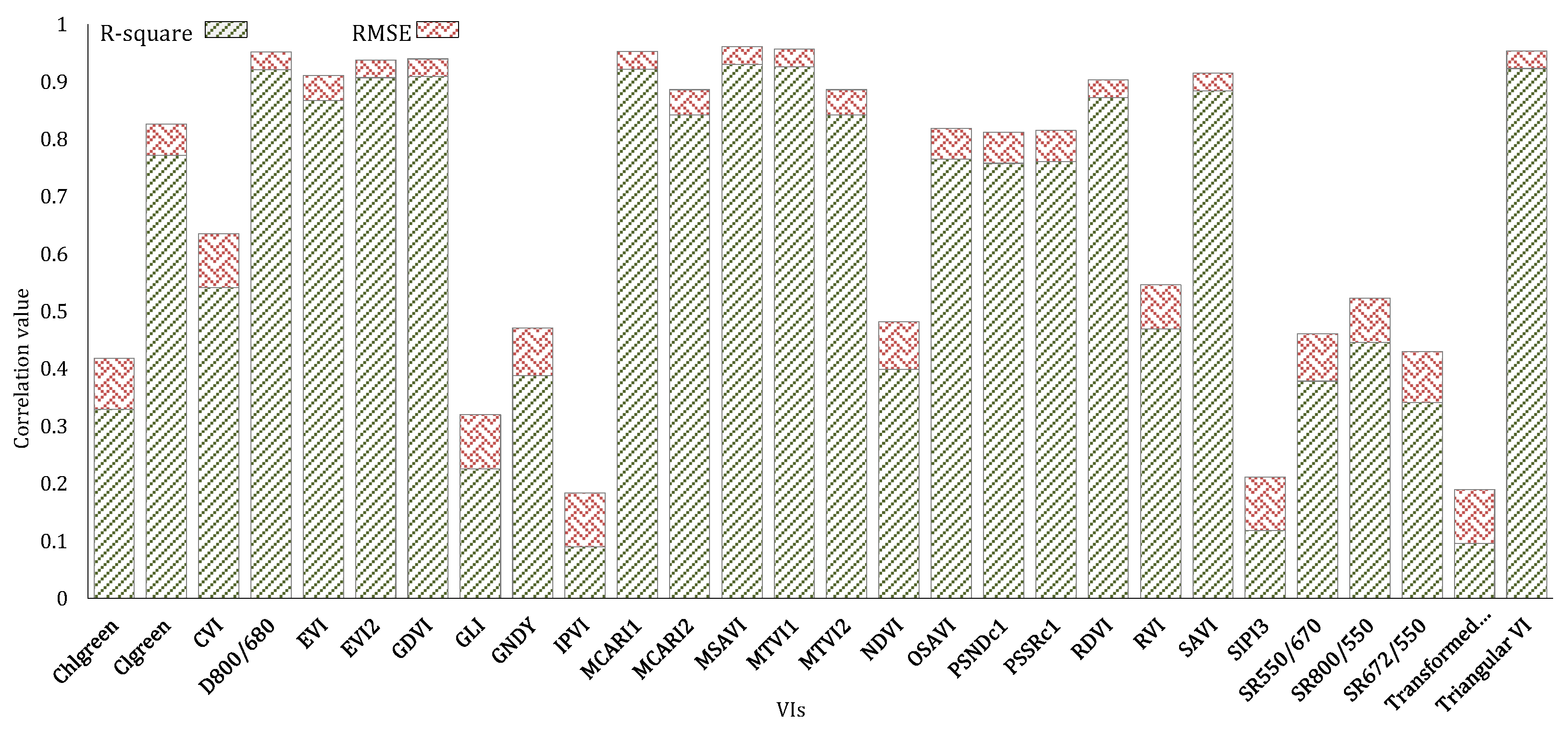
Figure 6.
Result of curve-fitting for MSAVI. MSAVI: modified soil-adjusted vegetation index.


Table 1.
Summary of the reviewed research works on satellite sensors used in nitrogen management in agriculture.
Table 1.
Summary of the reviewed research works on satellite sensors used in nitrogen management in agriculture.
| Satellite Sensor | Application | Indices | Correlation | Reference |
|---|---|---|---|---|
| IKONOS | Nitrogen detection in rice | > 0.9 | [24] | |
| QuickBird | Detect the biophysical and biochemical characteristics of potato (predicting the amount of nitrogen) | MSAVI | > 0.9 | [25] |
| QuichBird | Evaluate the status of N in winter wheat (Correlation between satellite images and the amount of N concentration) | all broadband indices | > 0.9 | [26] |
| RapidEye | to predict N status of spring wheat | MCARI/MTVI2 | [27] | |
| RapidEye | measure the amount of N in the wheat leaf (Finding a relationship between RapidEye satellite imagery and SPAD | NDRE/NDVI | 0.77 | [28] |
| Aster | predicted corn canopy N content by generating N fertilization map using SAM | MTVI2 | 0.87 | [29] |
| RapidEye | estimated the status of N in almond | NDVI and CCCI | > 0.9 | [30] |
| WorldView-2 | Monitored the N concentration and the amount of C in forest trees | SVM and ANN | > 0.9 | [31] |
SPAD: soil–plant analysis development; SAM: spectral angle mapper MSAVI: modified soil-adjusted vegetation index; MCARI/MTVI2: the ratio of the modii ed chlorophyll absorption ratio index to the second modii ed triangular vegetation index; NDRE/NDVI: the normalized difference red edge index to normalized difference vegetation index CCCI: canopy chlorophyll content index SVM: support vector machines; ANN: artificial neural network.
Table 2.
The trial layout of the study area and the different agricultural practices.
| Trial Site Code | FASSB PPPTR | ||
|---|---|---|---|
| Plot Size | 6 × 8 Palms (4 × 6 recorded) | ||
| No. of Plot | 18 Plots (3 treatments × 6 replication) | ||
| Trial Design | RCBD | ||
| Land Area | 6.35 ha | ||
| Planting Material | D × P Yangambi (ML 161) | ||
| Soil Series | Katong | ||
| Terrain | Moderately Undulating | ||
| Coordinate points | Top Left: Lat: 3°54′41.84″ N Lon: 102°31′46.38″ E | Top Right: Lat: 3°54′41.80″ N Lon: 102°32′8.02″ E | |
| Down Left: Lat: 3°54′35.59″ N Lon: 102°31′46.71″ E | Down Right: Lat: 3°54′35.68″ N Lon: 102°32′7.99″ E | ||
| Treatment | A Good Agronomic Practice | B Standard Practice | C Sub-Standard |
| Plowing | ✓ Planting row | X | X |
| Liming | ✓ 2 t/ha | X | X |
| Legume | ✓ Mb: CM: Pj | ✓ Mb | X |
| Mulching | ✓ FM + compost | ✓ Chipping | X |
| Ablation | ✓ 4 times | ✓ 2 times | X |
RCBD: randomized complete block design.
Table 3.
Fertilizer schedule in 2015 and 2016.
| 2015 | |||
| Round | Fert. Type | Rate kg per Tree | Date Applied |
| 1 | CPD | 3.00 | 17 April |
| 2 | NK Mix | 1.50 | 7 Jun |
| 3 | CPD | 2.75 | 29 August |
| 4 | NK Mix | 1.50 | 15 November |
| Sum = 8.75 | |||
| 2016 | |||
| 1 | NK Mix | 2.25 | 25 April |
| 2 | CPD | 1.00 | 20 May |
| 3 | NK Mix | 2.00 | 15 August |
| 4 | GML * | 2.50 | 9 October |
| 5 | NK Mix | 2.00 | 22 November |
| Sum = 9.75 | |||
* GML: ground magnesium limestone. CPD: Compound fertilizers.
Table 4.
SPOT-7 satellite sensor specifications.
| Specification | Description |
|---|---|
| Launch Date | 30 June 2014 |
| Spectral Bands | Panchromatic: 0.450–0.745 mm Blue (0.455–0.525 µm) Green (0.530–0.590 µm) Red (0.625–0.695 µm) Near-Infrared (0.760–0.890 µm) |
| Resolution (GSD) | Panchromatic-1.5m Multispectral 6.0 m (B,G,R,NIR) |
| Imaging Swath | 60 km at Nadir |
| Altitude | 694 km |
| Bit Depth | 12 bits per pixel (4096 values) |
| Detectors | PAN array assembly: 28,000 pixels MS array assembly: 4 × 7000 pixels |
| Revisit | 1 day with SPOT-6 and SPOT-7 operating simultaneously between 1 and 3 days with only one satellite in operation |
Table 5.
Different vegetation indices.
| No. | Vegetation Indices | Common Name | Equation | Reference |
|---|---|---|---|---|
| 1 | Chlorophyll Green | Chlgreen | [41] | |
| 2 | Chlorophyll Index Green | CIgreen | [42] | |
| 3 | Chlorophyll Vegetation Index | CVI | [43] | |
| 4 | Difference 800/680 | D800/680 | [44] | |
| 5 | Enhanced Vegetation Index | EVI | [45] | |
| 6 | Enhanced Vegetation Index 2 | EVI2 | [46] | |
| 7 | Difference NIR/Green Green Difference Vegetation Index | GDVI | [47] | |
| 8 | Green Leaf Index | GLI | [48] | |
| 9 | Normalized Difference NIR/Green Green NDVI | GNDVI | [49] | |
| 10 | Infrared Percentage Vegetation index | IPVI | [50] | |
| 11 | Modified Chlorophyll Absorption in Reflectance Index 1 | MCARI1 | [51,52] | |
| 12 | Modified Chlorophyll Absorption in Reflectance Index 2 | MCARI2 | [51,53] | |
| 13 | Modified Soil Adjusted Vegetation Index | MSAVI | [54] | |
| 14 | Modified Triangular Vegetation Index 1 | MTVI1 | [53] | |
| 15 | Modified Triangular Vegetation Index 2 | MTVI2 | [53] | |
| 16 | Normalized Difference Vegetation Index | NDVI | [55] | |
| 17 | Optimized Soil Adjusted Vegetation Index | OSAVI | [56] | |
| 18 | Normalized Difference 800/500 Pigment Specific Normalized Difference C1 | PSNDc1 | [57] | |
| 19 | Simple Ratio 800/500 Pigment Specific Simple Ratio C1 | PSSRc1 | [57] | |
| 20 | Renormalized Difference Vegetation Index | RDVI | [58] | |
| 21 | Simple Ratio 800/670 Ratio Vegetation Index | RVI | [59] | |
| 22 | Soil Adjusted Vegetation Index | SAVI | [55] | |
| 23 | Structure Intensive Pigment Index 3 | SIPI3 | [60] | |
| 24 | Simple Ratio 550/670 | SR550/670 | [61] | |
| 25 | Simple Ratio 800/550 | SR800/550 | [62] | |
| 26 | Simple Ratio 672/550 Datt5 | SR672/550 | [63] | |
| 27 | Transformed Vegetation Index | TVI | [64] | |
| 28 | Triangular Vegetation Index | TVI | [55] |
Table 6.
Leaf sampling results.
| Sample Description | Parameters | Covariance | ||||||||
|---|---|---|---|---|---|---|---|---|---|---|
| Total-N | P | K | Mg | |||||||
| (%) | (%) | (%) | (%) | |||||||
| R1/A | 2.96 | 0.167 | 1.171 | 0.290 | 63.67 | |||||
| R2/A | 3.18 | 0.172 | 1.170 | 0.344 | 66.88 | 70.25 | ||||
| R3/A | 2.99 | 0.166 | 1.004 | 0.302 | 51.30 | 53.89 | 41.38 | |||
| R4/A | 3.09 | 0.167 | 1.131 | 0.290 | 54.34 | 57.08 | 43.82 | 46.41 | ||
| R5/A | 2.94 | 0.165 | 0.978 | 0.286 | 54.53 | 57.28 | 43.97 | 46.51 | 46.72 | |
| R6/A | 3.03 | 0.167 | 0.840 | 0.263 | 54.62 | 57.38 | 44.05 | 46.65 | 46.81 | 46.9 |
| mean | 3.03 | 0.167 | 1.049 | 0.296 | ||||||
| Standard Dev | 0.0902 | 0.0024 | 0.1319 | 0.0268 | ||||||
| %CV | 2.97 | 1.43 | 12.57 | 9.05 | ||||||
| R1/B | 3.03 | 0.168 | 1.068 | 0.330 | 64.08 | |||||
| R2/B | 3.07 | 0.167 | 1.077 | 0.377 | 70.36 | 77.27 | ||||
| R3/B | 3.22 | 0.174 | 1.007 | 0.339 | 64.02 | 70.29 | 63.96 | |||
| R4/B | 3.12 | 0.167 | 1.105 | 0.306 | 54.51 | 59.84 | 54.47 | 46.40 | ||
| R5/B | 3.07 | 0.167 | 0.936 | 0.279 | 54.69 | 60.04 | 54.65 | 46.56 | 46.71 | |
| R6/B | 3.10 | 0.167 | 1.181 | 0.333 | 63.96 | 70.23 | 63.89 | 54.41 | 54.59 | 63.84 |
| mean | 3.10 | 0.168 | 1.062 | 0.327 | ||||||
| Standard Dev | 0.0841 | 0.0028 | 0.0838 | 0.0329 | ||||||
| %CV | 2.71 | 1.66 | 7.89 | 10.06 | ||||||
| R1/C | 2.99 | 0.165 | 1.193 | 0.343 | 57.71 | |||||
| R2/C | 3.12 | 0.170 | 1.190 | 0.325 | 63.70 | 70.31 | ||||
| R3/C | 2.99 | 0.165 | 0.993 | 0.355 | 51.88 | 57.26 | 46.64 | |||
| R4/C | 3.04 | 0.168 | 1.061 | 0.307 | 57.82 | 63.82 | 51.98 | 57.93 | ||
| R5/C | 2.97 | 0.163 | 0.912 | 0.280 | 52.01 | 57.41 | 46.76 | 52.12 | 46.89 | |
| R6/C | 2.99 | 0.167 | 1.067 | 0.282 | 48.82 | 53.88 | 43.90 | 48.92 | 44.02 | 41.33 |
| mean | 3.01 | 0.166 | 1.069 | 0.315 | ||||||
| Standard Dev | 0.1068 | 0.0025 | 0.11 | 0.0311 | ||||||
| %CV | 3.54 | 1.5 | 10.28 | 9.87 | ||||||
Table 7.
Percentages of nutrient concentration in oil palm leaves (over 6 years).
| Nutrient | Deficiency | Marginal | Optimum | Marginal | Excess |
|---|---|---|---|---|---|
| N | < 2.3 | 2.3 to 2.4 | 2.4 to 2.80 | 2.8 to 3 | > 3 |
| P | < 0.14 | 0.14 to 0.15 | 0.15 to 0.18 | 0.18 to 0.25 | > 0.25 |
| K | < 0.75 | 0.75 to 0.9 | 0.9 to 1.2 | 0.9 to 1.6 | > 1.6 |
| Mg | < 0.2 | 0.2 to 0.25 | 0.25 to 0.4 | 0.4 to 0.7 | > 0.7 |
Table 8.
Model summary of modified soil-adjusted vegetation index (MSAVI) in SPSS software.
| Model Name | Model Summary | |||
|---|---|---|---|---|
| R | R-Square | Adjusted R-Square | Std. Error of the Estimate | |
| Linear | 0.070 | 0.005 | −0.137 | 0.099 |
| Logarithmic | 0.022 | 0.000 | −0.142 | 0.099 |
| Quadratic | 0.964 | 0.930 | 0.906 | 0.028 |
| Compound a | 0.063 | 0.004 | −0.138 | 0.032 |
| Power a | 0.015 | 0.000 | −0.143 | 0.032 |
| S a | 0.032 | 0.001 | −0.142 | 0.032 |
| Growth a | 0.063 | 0.004 | −0.138 | 0.032 |
| Exponential a | 0.063 | 0.004 | −0.138 | 0.032 |
| Independent Variable | MSAVI | |||
| Constant | Included | |||
| Variable Whose Values Label Observations in Plots | Unspecified | |||
| Tolerance for Entering Terms in Equations | 0.0001 | |||
a The model requires all non-missing values to be positive. MSAVI: modified soil-adjusted vegetation index.
Table 9.
Analysis of variance of the modified soil adjusted vegetation index.
| Sum of Squares | Degrees of Freedom (DF) | Mean Square | F ratio | p-value. | |
| Regression | 0.064 | 2 | 0.032 | 39.657 | 0.000 |
| Residual | 0.005 | 6 | 0.001 | ||
| Total | 0.069 | 8 | |||
| Coefficients of MSAVI | |||||
| Unstandardized Coefficients | Standardized Coefficients Beta | t | p-value. | ||
| B | Std. Error | ||||
| MSAVI_9S | −12.921 | 1.462 | −19.228 | −8.839 | 0.000 |
| MSAVI_9S ** 2 | 4.145 | 0.467 | 19.322 | 8.882 | 0.000 |
| (Constant) | 13.052 | 1.138 | 11.467 | 0.000 | |
Table 10.
Predicted nitrogen concentration (%).
| Plot | MSAVI | Actual N (%) | Plot | MSAVI | Actual N (%) | Predicted N (%) |
|---|---|---|---|---|---|---|
| 1B | 1.556866655748 | 3.03 | 6B | 1.755091701945 | 3.10 | 3.14 |
| 1C | 1.497733329733 | 2.99 | 6C | 1.673120826483 | 2.99 | 3.04 |
| 1A | 1.572449992101 | 2.96 | 6A | 1.671252056957 | 3.03 | 3.04 |
| 2C | 1.364485422771 | 3.12 | 5C | 1.559139554700 | 2.97 | 2.98 |
| 2A | 1.360270857811 | 3.18 | 5A | 1.502304171522 | 2.94 | 3.00 |
| 2B | 1.400625000397 | 3.07 | 5B | 1.500858326754 | 3.07 | 3.00 |
| 3A | 1.485445639362 | 2.99 | 4A | 1.435083339612 | 3.09 | 3.05 |
| 3B | 1.799166644614 | 3.22 | 4B | 1.754893735051 | 3.12 | 3.14 |
| 3C | 1.597421970367 | 2.99 | 4C | 1.489568730196 | 3.04 | 3.00 |
MSAVI: modified soil-adjusted vegetation index.
Table 11.
Group statistic independent t-test.
| Group Independen t-test | N | Mean | Std. Deviation | Std. Error Mean | |
|---|---|---|---|---|---|
| Independent t-test | 1 | 9 | 3.0389 | 0.06214 | 0.02071 |
| 2 | 9 | 3.0433 | 0.05958 | 0.01986 | |
Table 12.
Levene’s test for testing the equality of variances.
| Levene’s Test for Equality of Variances | t-test for Equality of Means | |||||||||
|---|---|---|---|---|---|---|---|---|---|---|
| F | Sig. | t | df | Sig. (2-tailed) | Mean Difference | Std. Error Difference | 95% Confidence Interval of the Difference | |||
| Lower | Upper | |||||||||
| Independent t-test | Equal variances assumed | 0.123 | 0.731 | −0.155 | 16 | 0.879 | −0.00444 | 0.02870 | −0.06528 | 0.05639 |
| Equal variances not assumed | −0.155 | 15.97 | 0.879 | −0.00444 | 0.02870 | −0.06529 | 0.05640 | |||
Table 13.
Classification accuracy for the percentage of oil palm leaf nitrogen content.
| MSAVI | Actual N% | Predicted | Three-level N Content | ||
|---|---|---|---|---|---|
| Actual | Predicted | True/false | |||
| 1.755091701945 | 3.10 | 3.14 | Excess | Excess | 1 |
| 1.673120826483 | 2.99 | 3.04 | Marginal | Excess | 0 |
| 1.671252056957 | 3.03 | 3.04 | Excess | Excess | 1 |
| 1.559139554700 | 2.97 | 2.98 | Marginal | Marginal | 1 |
| 1.502304171522 | 2.94 | 3.00 | Marginal | Excess | 0 |
| 1.500858326754 | 3.07 | 3.00 | Excess | Excess | 1 |
| 1.435083339612 | 3.09 | 3.05 | Excess | Excess | 1 |
| 1.754893735051 | 3.12 | 3.14 | Excess | Excess | 1 |
| 1.489568730196 | 3.04 | 3.00 | Excess | Excess | 1 |
| Total Sample | 9 | ||||
| Percent of true (Accuracy) | 77.7% | ||||
MSAVI: modified soil-adjusted vegetation index.
© 2020 by the authors. Licensee MDPI, Basel, Switzerland. This article is an open access article distributed under the terms and conditions of the Creative Commons Attribution (CC BY) license (http://creativecommons.org/licenses/by/4.0/).
Share and Cite
MDPI and ACS Style
Yadegari, M.; Shamshiri, R.R.; Mohamed Shariff, A.R.; Balasundram, S.K.; Mahns, B. Using SPOT-7 for Nitrogen Fertilizer Management in Oil Palm. Agriculture 2020, 10, 133. https://doi.org/10.3390/agriculture10040133
AMA Style
Yadegari M, Shamshiri RR, Mohamed Shariff AR, Balasundram SK, Mahns B. Using SPOT-7 for Nitrogen Fertilizer Management in Oil Palm. Agriculture. 2020; 10(4):133. https://doi.org/10.3390/agriculture10040133
Chicago/Turabian StyleYadegari, Mohammad, Redmond R. Shamshiri, Abdul Rashid Mohamed Shariff, Siva K. Balasundram, and Benjamin Mahns. 2020. "Using SPOT-7 for Nitrogen Fertilizer Management in Oil Palm" Agriculture 10, no. 4: 133. https://doi.org/10.3390/agriculture10040133
Note that from the first issue of 2016, this journal uses article numbers instead of page numbers. See further details here.