Experimental Verification of Methods for Converting Acceleration Data in High-Rise Buildings into Displacement Data by Shaking Table Test


Abstract
:1. Introduction
2. Experimental Setup and Processing Methods
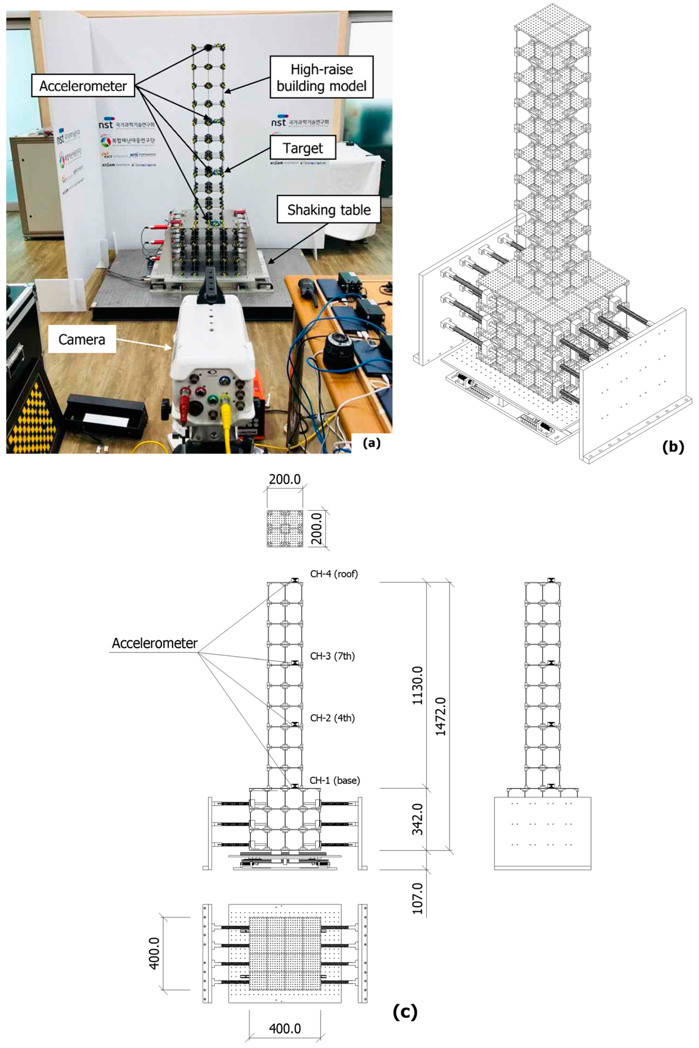
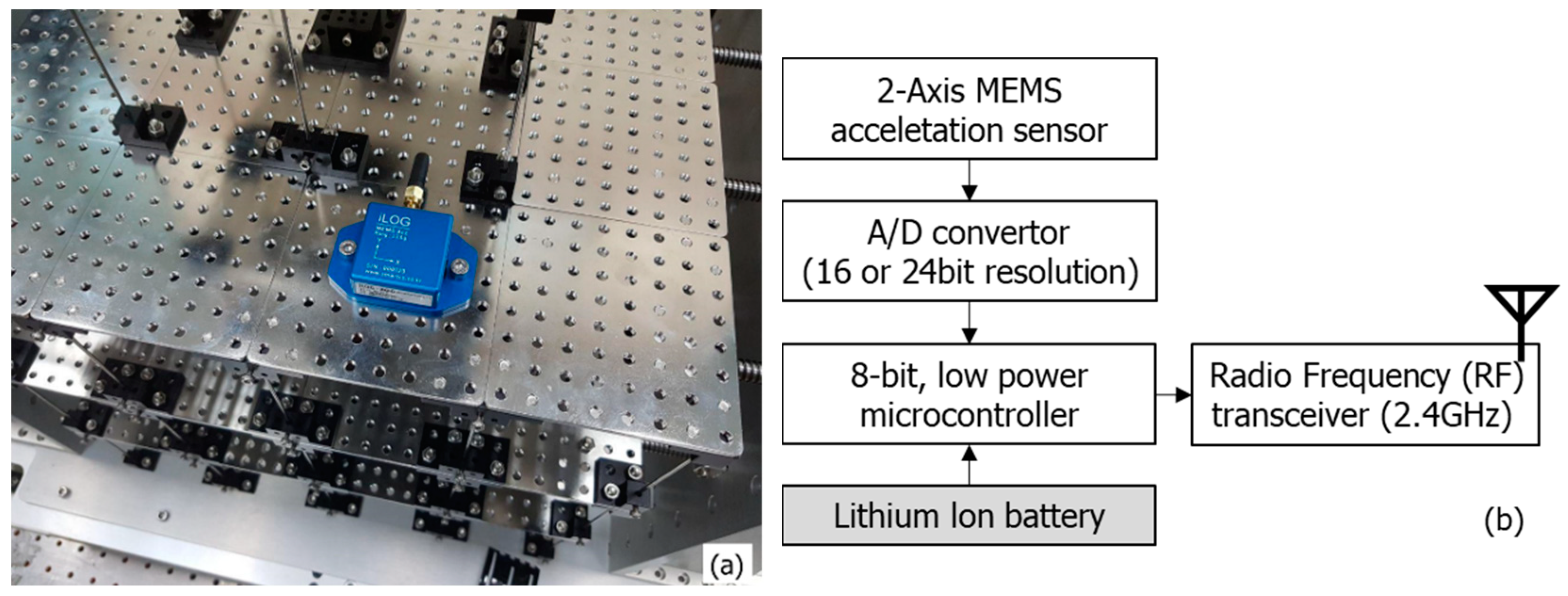
2.1. Shaking Table Test
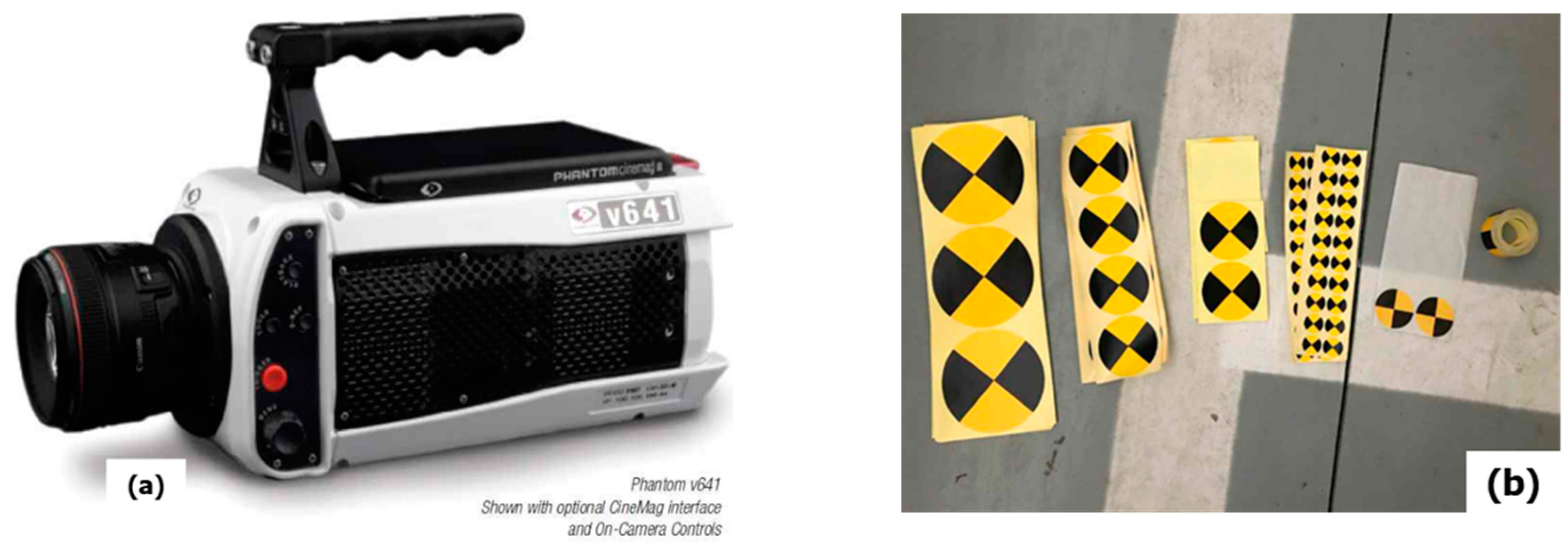
2.2. High-Speed Camera Shooting and Image Analysis
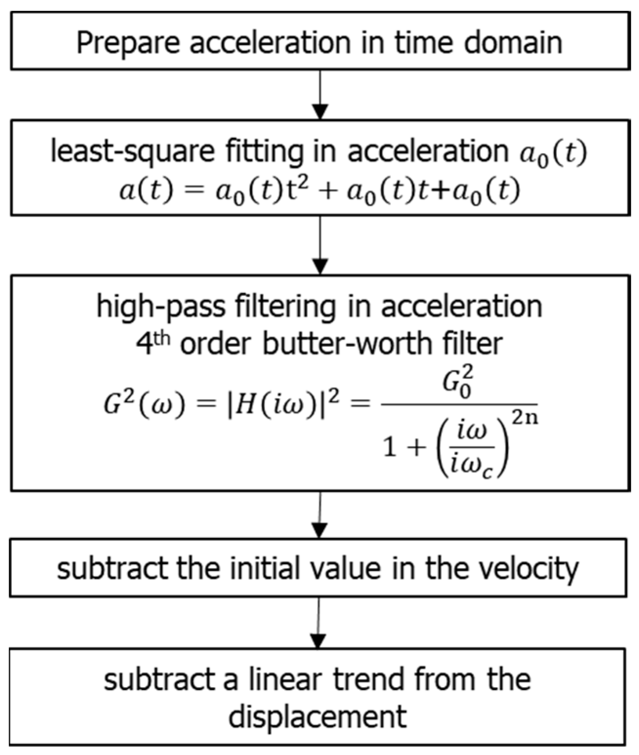
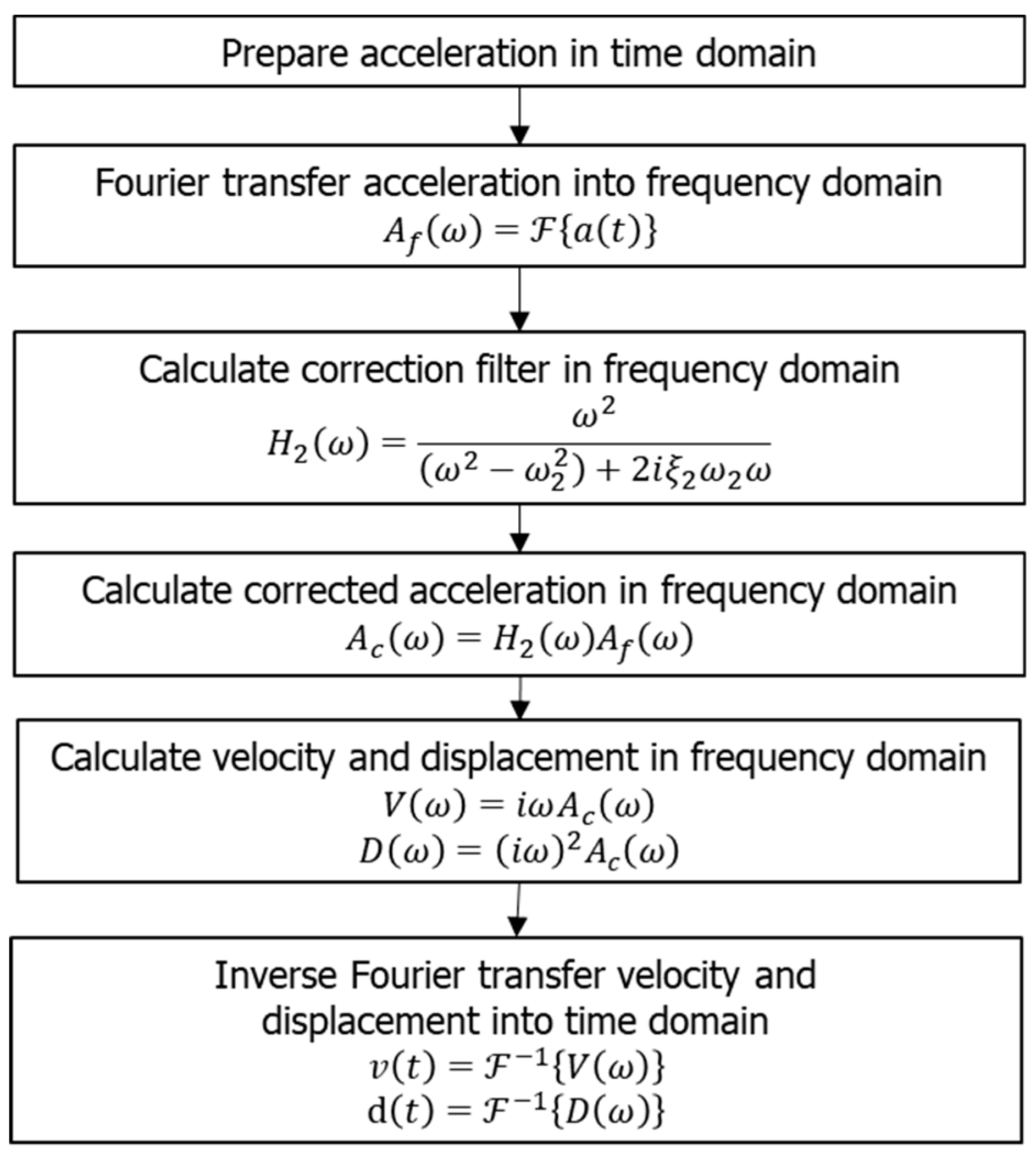
2.3. AVD Conversion Method
3. Shaking Table Test
3.1. Test Conditions
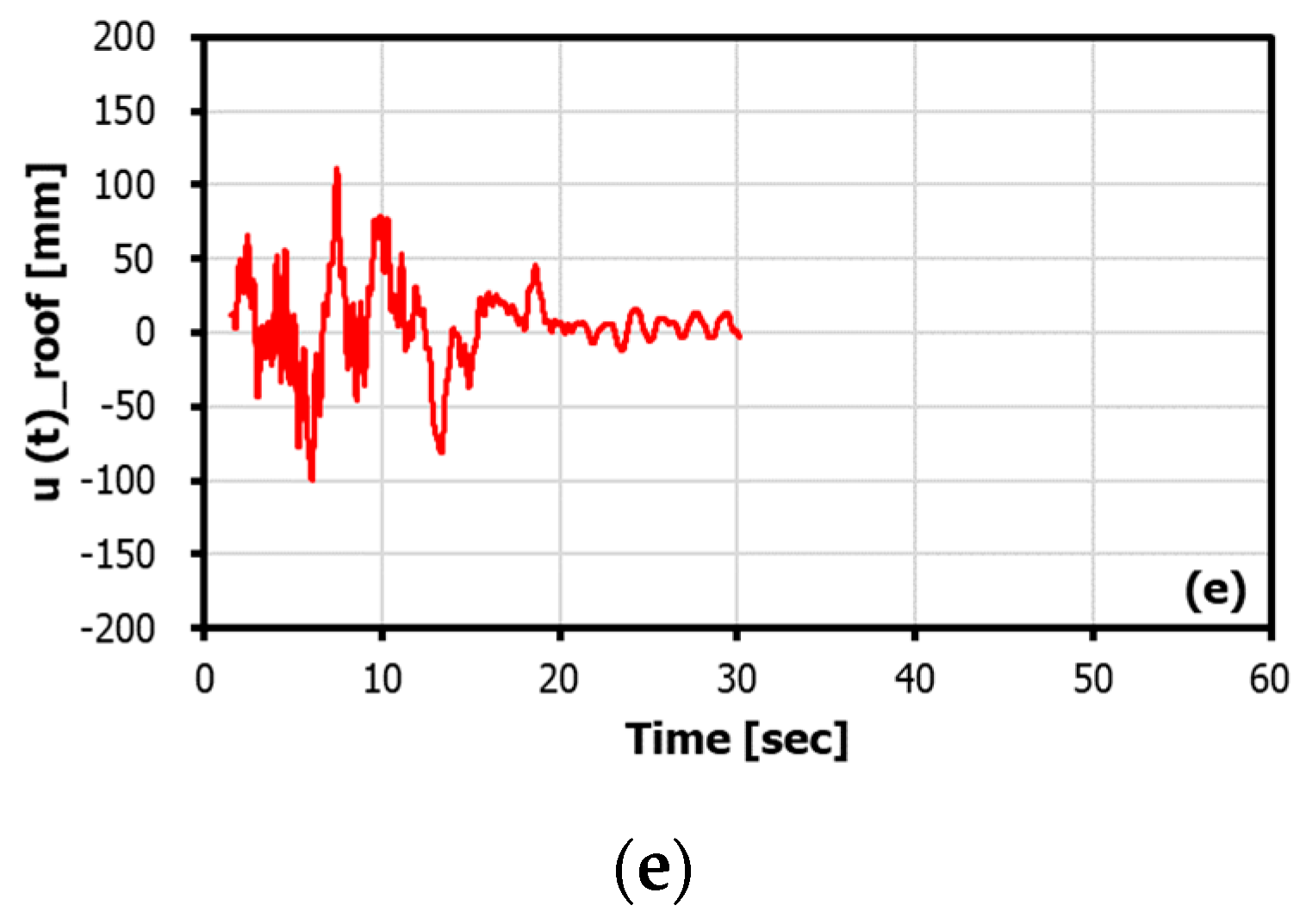
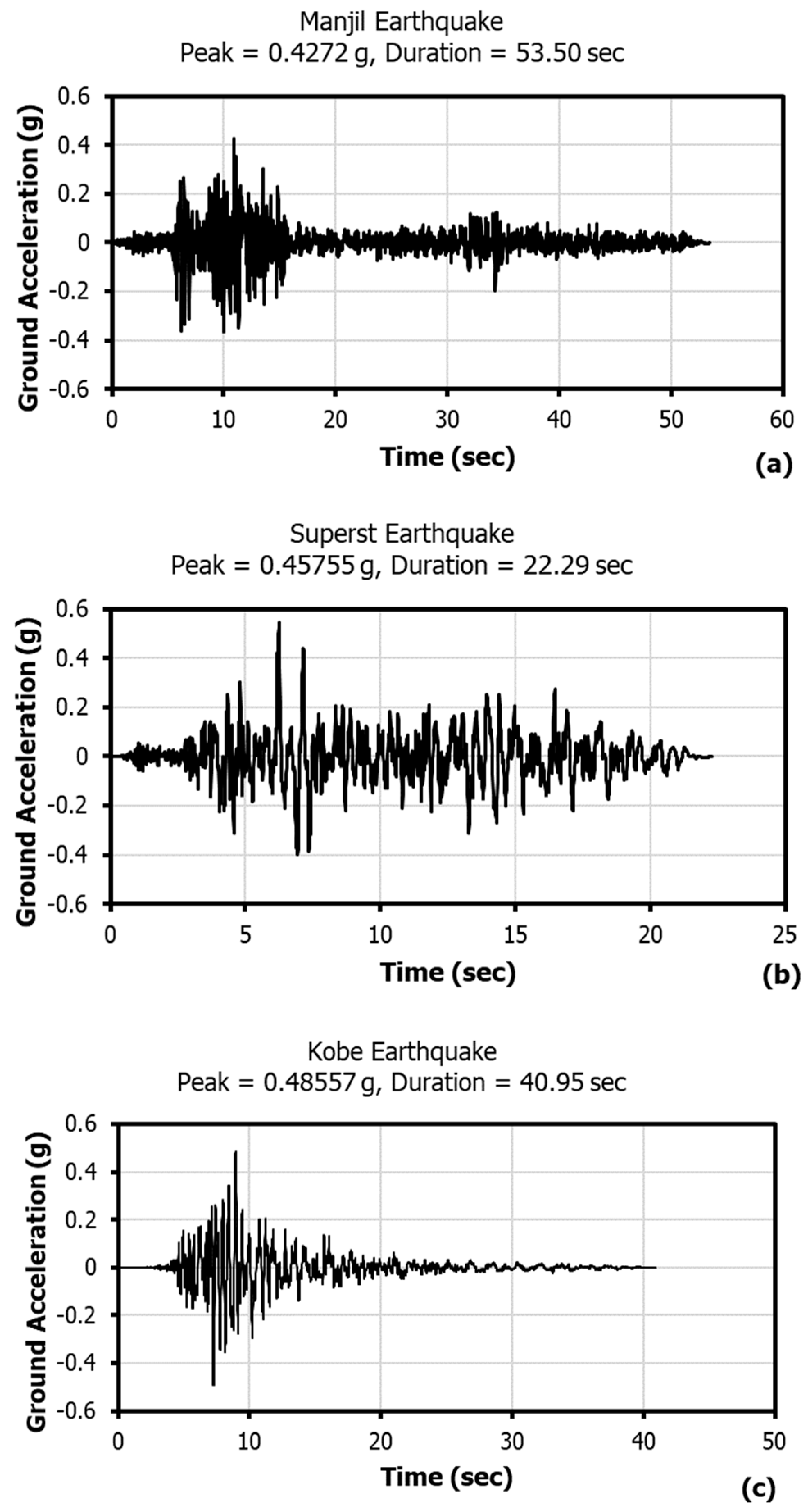
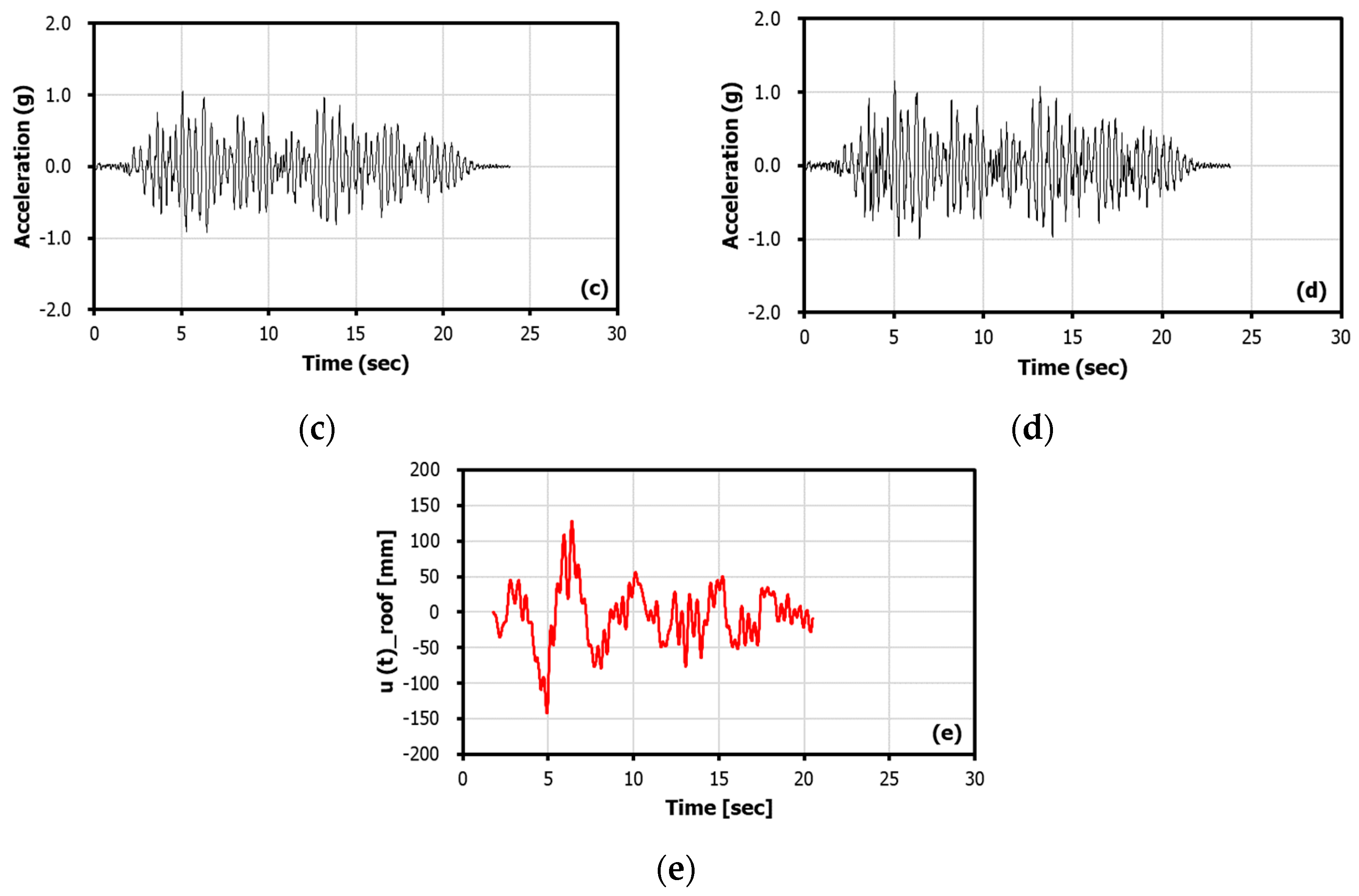
3.2. Experimental Response with Application of Strong Motion
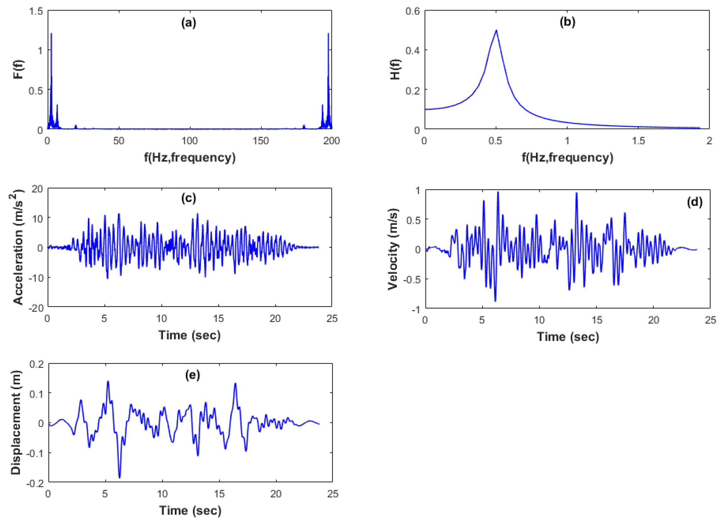
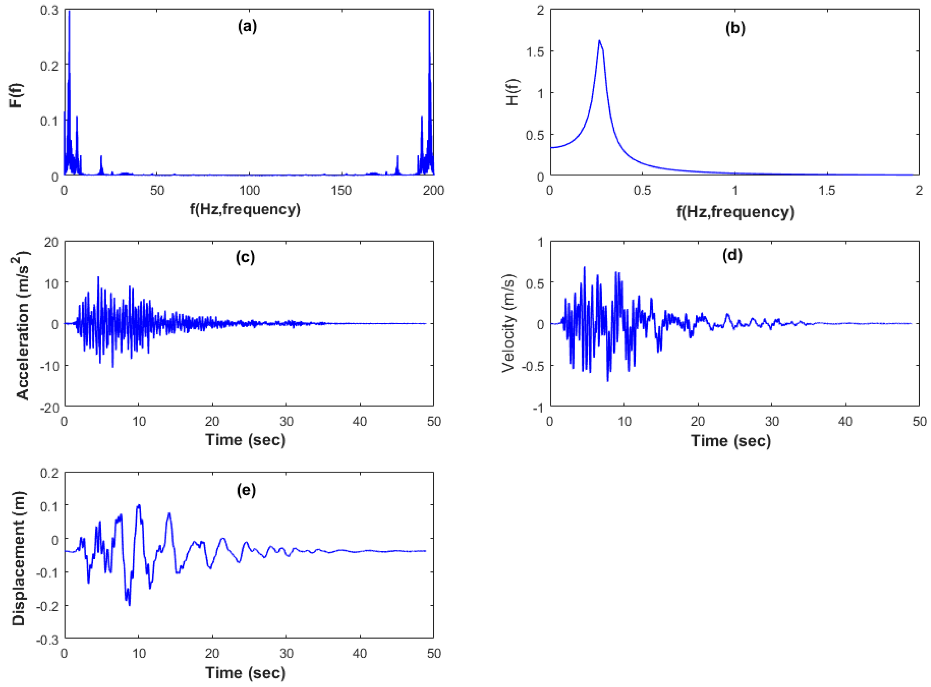
3.3. Conversion Process of Each Method
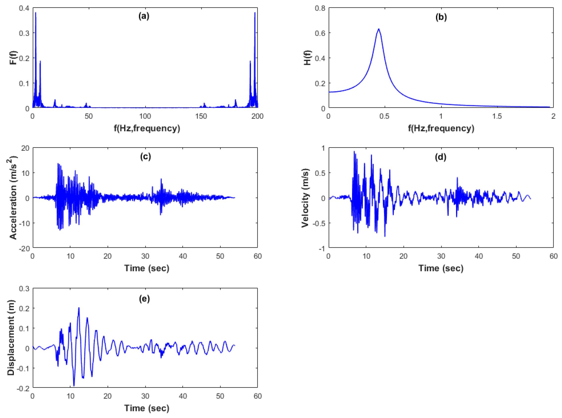
3.3.1. Method 1
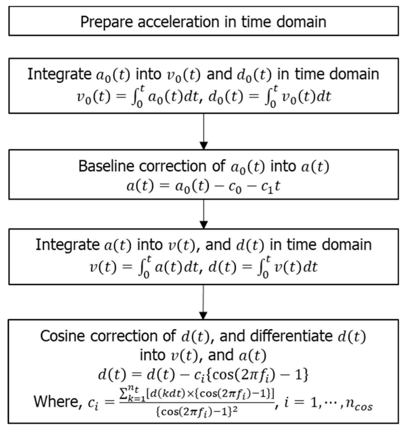
3.3.2. Method 2
3.3.3. Method 3
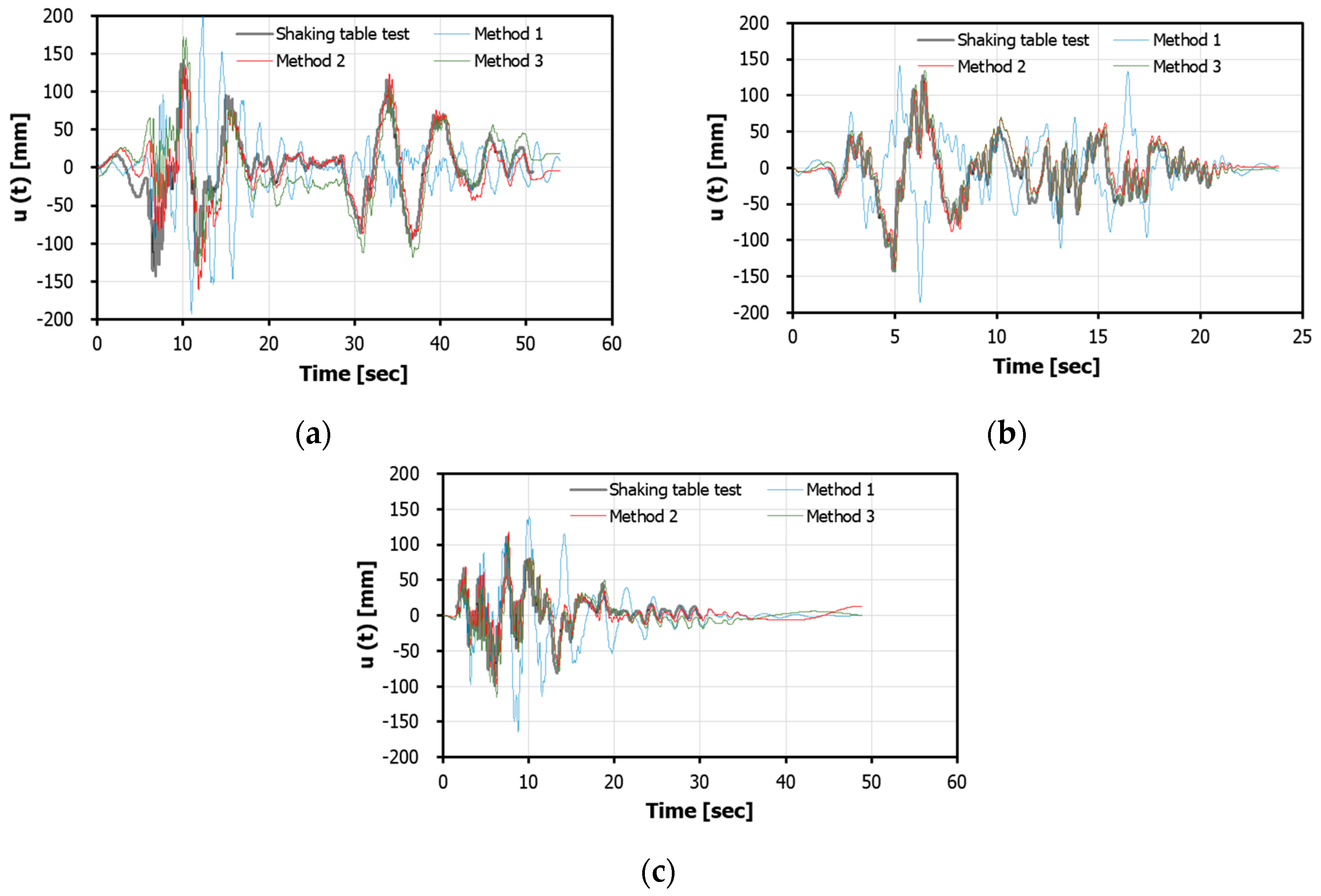
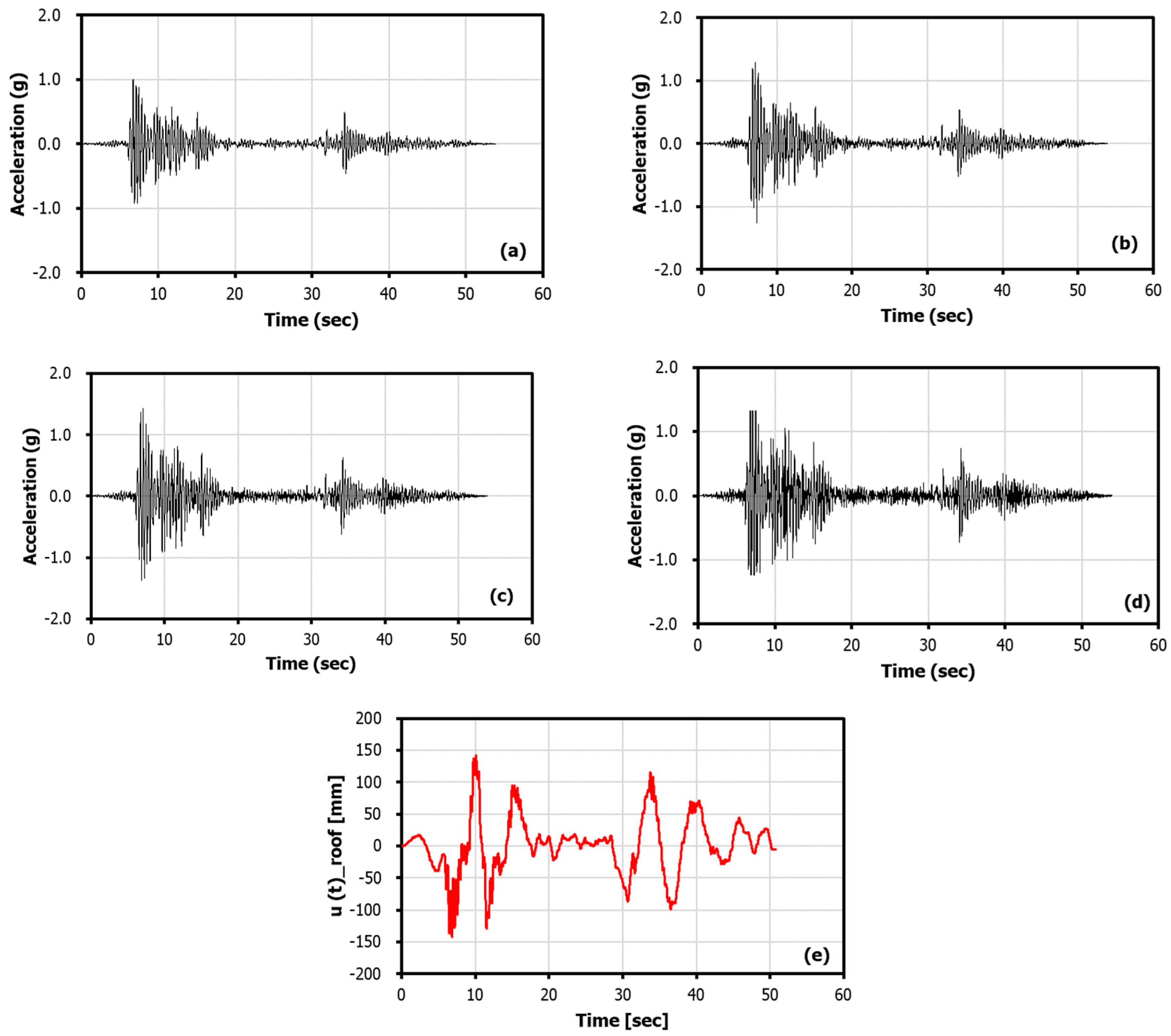
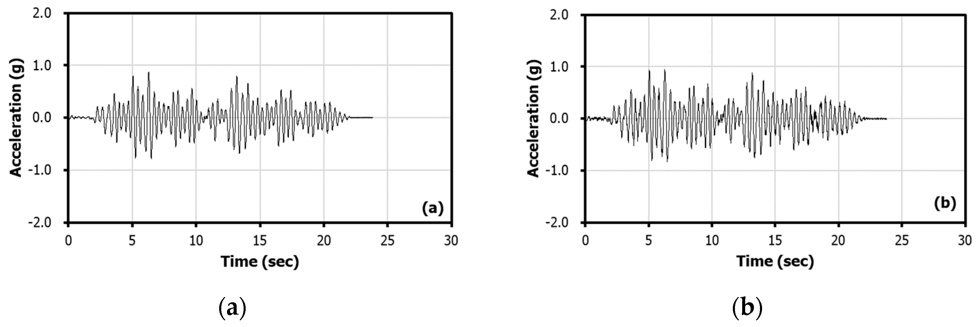
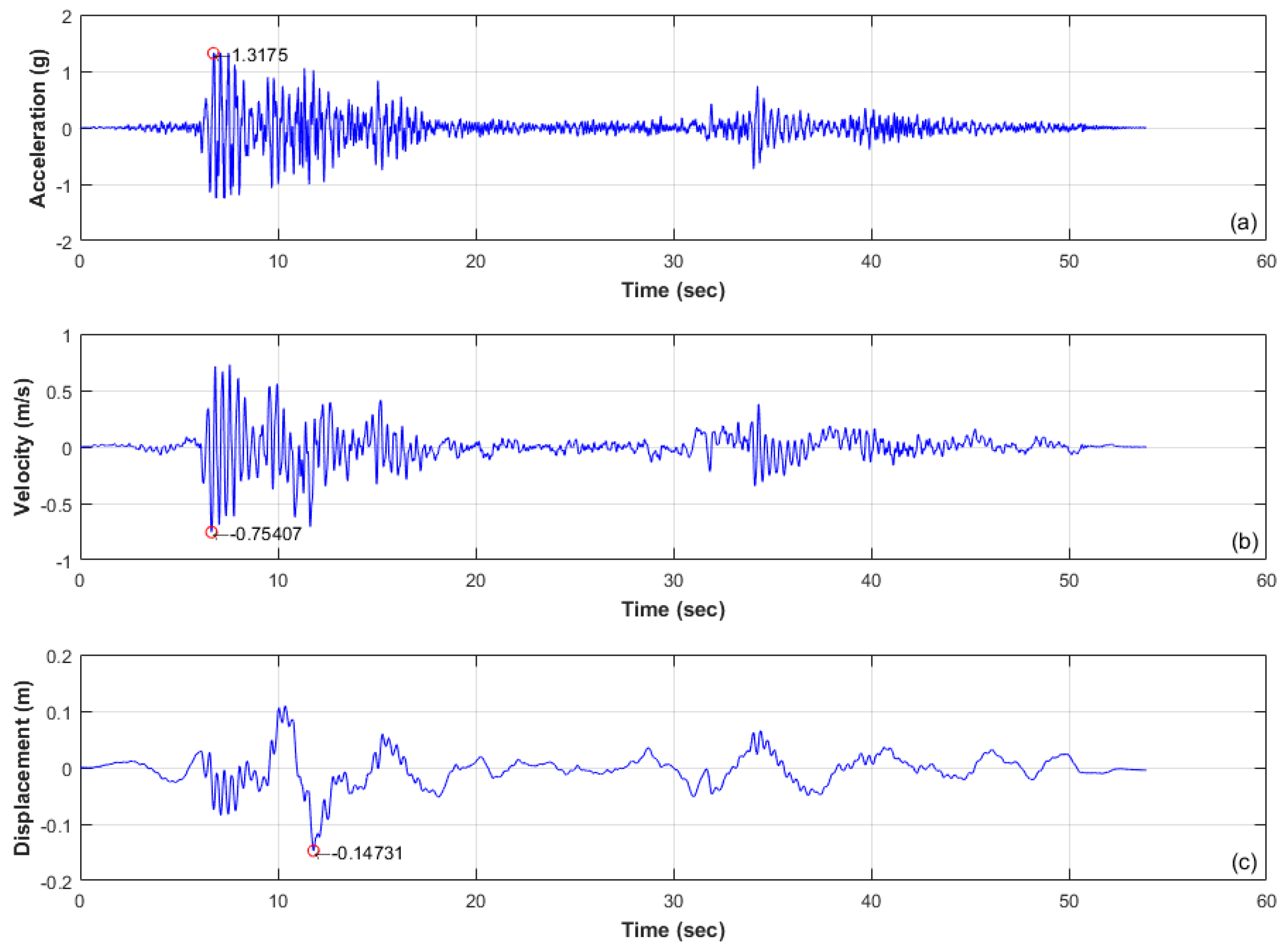
3.4. Comparison of Acceleration Data Converted to Velocity and Displacement
4. Conclusions
- First step: A technique is required to establish a fixed point, so that the integration of acceleration data will not be subject to accumulated errors.
- Second step: Methods for eliminating baseline drift are also taken into consideration, including baseline correction filters and least-square fitting. These could be referred to as a first filter.
- Third step: After these 2 steps, the noise contained in the real data needs to be eliminated. This step is the most important step. There are many potential second filters, including discrete Fourier transformation (Method 1), the cosine correction filter (Method 2), and the Butterworth filter (Method 3).
Author Contributions
Funding
Acknowledgments
Conflicts of Interest
References
- Darragh, B.; Silva, W.; Gregor, N. Strong motion record processing for the PEER center. In Proceedings of the COSMOS Invited Workshop on Strong-Motion Record Processing, Richmond, CA, USA, 26–27 May 2004; pp. 26–27. [Google Scholar]
- Mollova, G. Effects of digital filtering in data processing of seismic acceleration records. Eurasip J. Adv. Signal Process. 2007, 2007, 029502. [Google Scholar] [CrossRef]
- Ambraseys, N.; Smit, P.; Douglas, J.; Margaris, B.; Sigbjörnsson, R.; Olafsson, S.; Suhadolc, P.; Costa, G. Internet site for European strong-motion data. Boll. Geofis. Teor. Appl. 2004, 45, 113–129. [Google Scholar]
- Jones, J.; Kalkan, E.; Stephens, C.; Ng, P. Prism, processing and review interface for strong motion data software. In Eleventh U.S. National Conference on Earthquake Engineering; Integrating Science, Engineering & Policy: Los Angeles, CA, USA, 2018. [Google Scholar]
- Jones, J.; Kalkan, E.; Stephens, C. Processing and Review Interface for Strong Motion Data (Prism) Software, Version 1.0. 0—Methodology and Automated Processing; 2331-1258; US Geological Survey: Reston, VA, USA, 2017.
- Jones, J.; Kalkan, E.; Stephens, C.; Ng, P.J.S.R.L. PRISM Software: Processing and Review Interface for Strong-Motion Data. Seismol. Res. Lett. 2017, 88, 851–866. [Google Scholar] [CrossRef]
- Luzi, L.; Puglia, R.; Russo, E.; D’Amico, M.; Felicetta, C.; Pacor, F.; Lanzano, G.; Çeken, U.; Clinton, J.; Costa, G.J.S.R.L. The engineering strong-motion database: A platform to access pan-European accelerometric data. Seismol. Res. Lett. 2016, 87, 987–997. [Google Scholar] [CrossRef]
- Luzi, L.; Puglia, R.; Russo, E.; D’Amico, M.; Lanzano, G.; Pacor, F.; Felicetta, C. Engineering Strong-Motion database: a gateway to access European strong motion data. In Proceedings of the 16th World Conference on Earthquake Engineering, Santiago, Chile, 9–13 January 2017. [Google Scholar]
- Scordilis, E.; Theodoulidis, N.; Kalogeras, I.; Margaris, B.; Klimis, N.; Stewart, J.; Boore, D.; Seyhan, E.; Savvaidis, A.; Mylonakis, G. Strong Motion Database for Crustal Earthquakes in Greece and Surrounding Area. In Proceedings of the 16th European conference on “Earthquake Engineering”, Thessaloniki, Greece, 18–21 June 2018. [Google Scholar]
- Puglia, R.; Russo, E.; Luzi, L.; D’Amico, M.; Felicetta, C.; Pacor, F.; Lanzano, G. Strong-motion processing service: A tool to access and analyse earthquakes strong-motion waveforms. Bull. Earthq. Eng. 2018, 16, 2641–2651. [Google Scholar] [CrossRef]
- Butterworth, C.J.E. Filter approximation theory. Engineer 1930, 7, 536–541. [Google Scholar]
- Van Valkenburg, M.E. Analog Filter Design; Holt, Rinehart, and Winston: New York, NY, USA, 1982. [Google Scholar]
- Tsuchihashi, T.; Yasuda, M. Rapid Diagnosis Systems Using Accelerometers in Seismic Damage of Tall Buildings. Int. J. High Rise Build. 2017, 6, 207–216. [Google Scholar] [CrossRef]
- Chiu, H.-C. Stable baseline correction of digital strong-motion data. Bull. Seismol. Soc. Am. 1997, 87, 932–944. [Google Scholar]
- Chiu, H.-C. A Compatible Baseline Correction Algorithm for Strong-Motion Data. Terr. Atmos. Ocean. Sci. 2012, 23, 171–180. [Google Scholar] [CrossRef]
- Malhotra, P.K. Response spectrum of incompatible acceleration, velocity and displacement histories. Earthq. Eng. Struct. Dyn. 2001, 30, 279–286. [Google Scholar] [CrossRef]
- Pecknold, D.; Riddell, R. Effect of initial base motion on response spectra-closure. J. Eng. Mech. Div. Asce 1979, 105, 1057–1060. [Google Scholar]
- Pecknold, D.A.; Riddell, R. Effect of initial base motion on response spectra. J. Eng. Mech. Div. 1978, 104, 485–491. [Google Scholar]
- Athanasiou, A.; Oliveto, G.; Ponzo, F.J.E.S. Baseline correction of digital accelerograms from field testing of a seismically isolated building. Earthq. Spectra 2018, 34, 915–939. [Google Scholar] [CrossRef]
- Cherry, S. Earthquake ground motions: Measurement and characteristics. In Engineering Seismology and Earthquake Engineering; Soines, N., Ed.; Springer: Berlin/Heidelberg, Germany, 1974; p. 315. [Google Scholar]
- Agnew, D.C.; Berger, J. Vertical seismic noise at very low frequencies. J. Geophys. Res. Solid Earth 1978, 83, 5420–5424. [Google Scholar] [CrossRef]
- Crombie, D.D.; Hasselmann, K.; Sell, W. High-frequency radar observations of sea waves travelling in opposition to the wind. Bound. Layer Meteorol. 1978, 13, 45–54. [Google Scholar] [CrossRef]
- Kanai, K.; Tanaka, T. On microtremor VIII. Bull. Earthq. Res. Inst. Univ. Tokyo 1961, 39, 97–114. [Google Scholar]
- Metz, A.; Wolf, M.; Achermann, P.; Scholkmann, F. A new approach for automatic removal of movement artifacts in near-infrared spectroscopy time series by means of acceleration data. Algorithms 2015, 8, 1052–1075. [Google Scholar] [CrossRef]
- Boore, D.M.; Bommer, J.J. Processing of strong-motion accelerograms: Needs, options and consequences. Soil Dyn. Earthq Eng. 2005, 25, 93–115. [Google Scholar] [CrossRef]
- Park, S.; Park, H.; Kim, J.; Adeli, H.J.M. 3D displacement measurement model for health monitoring of structures using a motion capture system. Measurement 2015, 59, 352–362. [Google Scholar] [CrossRef]
- Kasai, K.; Ito, H.; Ooki, Y.; Hikino, T.; Kajiwara, K.; Motoyui, S.; Ozaki, H.; Ishii, M. Full scale shake table tests of 5-story steel building with various dampers. In Proceedings of the 7th International Conference on Urban Earthquake Engineering (7CUEE) & 5th International Conference on Earthquake Engineering (5ICEE), Tokyo, Japan, 3–5 March 2010; pp. 11–22. [Google Scholar]
- Lu, X.; Chen, Y.; Mao, Y. Shaking table model test and numerical analysis of a supertall building with high-level transfer storey. Struct. Des. Tall Spec. Build. 2012, 21, 699–723. [Google Scholar] [CrossRef]
- Lu, X.; Zou, Y.; Lu, W.; Zhao, B. Shaking table model test on shanghai world financial center tower. Earthq. Eng. Struct. Dyn. 2007, 36, 439–457. [Google Scholar] [CrossRef]
- Lu, X.; Lu, X.; Guan, H.; Ye, L. Collapse simulation of reinforced concrete high-rise building induced by extreme earthquakes. Earthq. Eng. Struct. Dyn. 2013, 42, 705–723. [Google Scholar] [CrossRef]
- Park, J.-W.; Sim, S.-H.; Jung, H.-J. Development of a wireless displacement measurement system using acceleration responses. Sensors 2013, 13, 8377–8392. [Google Scholar] [CrossRef] [PubMed]
- Clough, R.; Penzien, J. Dynamics of Structures, 3rd ed.; Computers & Structures, Inc.: Berkeley, CA, USA, 2003. [Google Scholar]
- Kim, D. Dynamics of Structures 4th; Goomi Book: Seoul, Korea, 2017. [Google Scholar]
- Park, B.C.; Jin, Y.J.; Lim, K.H.; Seong, J.Y.; Park, K.J. Development of the Public Bulidings Emergency Integrity Assessment Technology Using Seismic Acceleration Response Signal; National Disaster Management Institute: Seoul, Korea, 2012; pp. 1–292.
- Guorui, H.; Tao, L. Review on Baseline Correction of Strong-Motion Accelerogram. Int. J. Sci. Technol. Soc. 2015, 3, 309–314. [Google Scholar] [CrossRef]
- Boore, D.M.; Stephens, C.D.; Joyner, W.B. Comments on Baseline Correction of Digital Strong-Motion Data: Examples from the 1999 Hector Mine, California, Earthquake. Bull. Seismol. Soc. Am. 2002, 92, 1543–1560. [Google Scholar] [CrossRef]
- FEMA. Quantification of Building Seismic Performance Factors, FEMA P-695; Applied Technology Council for the Federal Emergency Management Agency: Washington, DC, USA, 2009.
- Ahn, S.-K.; Jeong, H.-I.; La, W. Estimation of Damping Ratio for Floor slabs of Building Structure. In Proceedings of the Korean Society for Noise and Vibration Engineering Conference, 2009; The Korean Society for Noise and Vibration Engineering: Seoul, Korea, 2009. [Google Scholar]


| Parameter | Specifications |
|---|---|
| Sensor input channels | Internal 2 or 3 axial MEMS ACC sensor |
| Resolution | 16 bit resolution |
| Dynamic range | 62.6 dB (typical) |
| MEMS Accelerometer Requirements | |
| Range | ±1.2 g, ±2.0 g, ±3.0 g, ±5.0 g |
| Sensitivity | 1000 mV/g, 420 mV/g, 300 mV/g, 174 mV/g |
| Noise Density | 110 μg/rtHz, 250 μg/rtHz, 300 μg/rtHz, 250 μg/rtHz |
| Sampling | |
| Measurable signal bandwidth | 0 Hz to 50 Hz (custom options available to 400 Hz) |
| Sampling rate | 50 to 1200 SPS, 2400 SPS (Via iLOG-RECEIVER) |
| Operating Parameters | |
| Wireless communication range | Outdoor: 200 m (typical) Indoor: 50 m (typical) |
| Radio frequency (RF) transceiver carrier | 2.4 Ghz to 2.4835 Ghz Bluetooth V2.0 + EDR Class 1 |
| RF communication protocol | IEEE 802.15.1 |
| RF Power | Max 18 dBm |
| Power source | Internal: 3.7 V 280 mA Li-po battery |
| Power consumption | 0.5 W (Active mode) |
| Duration | 2 h (Active mode) |
| Operating temperature | −20 °C to +60 °C |
| Physical Specifications | |
| Dimensions | 64 mm × 41.5 mm × 18 mm |
| Weight | 65 g |
| Enclosure material | Aluminum |
| Environmental rating | Indoor use |
| Equipment Name | Model Name (Manufacturer) | Special Feature | Amount |
|---|---|---|---|
| High-speed camera | Phantom V641 (Vision research) | As a device capable of shooting over 1000 frames per second, it captures moments that cannot be observed by the human eye and analyzes the behavior of the structure using these records. | Two sets |
| Target | Easy-to-perceive Quadrant target & linear target in TEMA software | 5 inch 3 inch 1 inch Linear | |
| Image analysis program | TEMA (Image systems) | A program which can analyze length, speed, acceleration, angle, angular velocity, etc., through a captured image or images | 1 EA |
| Method | Filter | Technique |
|---|---|---|
| 1 | Penzien filter | DFT Frequency-domain |
| 2 | Cosine correction filter | Zero padding Baseline correction (1st order) Cosine correction filter Time-domain |
| 3 | Butter-worth filter | Least-square fitting Butter-worth filter (4th order) Frequency-domain |
© 2019 by the authors. Licensee MDPI, Basel, Switzerland. This article is an open access article distributed under the terms and conditions of the Creative Commons Attribution (CC BY) license (http://creativecommons.org/licenses/by/4.0/).
Share and Cite
Han, H.; Park, M.; Park, S.; Kim, J.; Baek, Y. Experimental Verification of Methods for Converting Acceleration Data in High-Rise Buildings into Displacement Data by Shaking Table Test. Appl. Sci. 2019, 9, 1653. https://doi.org/10.3390/app9081653
Han H, Park M, Park S, Kim J, Baek Y. Experimental Verification of Methods for Converting Acceleration Data in High-Rise Buildings into Displacement Data by Shaking Table Test. Applied Sciences. 2019; 9(8):1653. https://doi.org/10.3390/app9081653
Chicago/Turabian StyleHan, Heuisoo, Mincheol Park, Sangki Park, Juhyong Kim, and Yong Baek. 2019. "Experimental Verification of Methods for Converting Acceleration Data in High-Rise Buildings into Displacement Data by Shaking Table Test" Applied Sciences 9, no. 8: 1653. https://doi.org/10.3390/app9081653