An Improved Objective Function for Modal-Based Damage Identification Using Substructural Virtual Distortion Method


1
Department of Civil Engineering & State Key Laboratory of Coastal and Offshore Engineering, Dalian University of Technology, Dalian 116023, China
2
Key Laboratory of Structures Dynamic Behavior and Control of Ministry of Education, Harbin Institute of Technology, Harbin 150090, China
3
Department of Civil Engineering, Dalian Minzu University, Dalian 116650, China
4
Institute of Fundamental Technological Research, Polish Academy of Sciences, 02-106 Warsaw, Poland
*
Author to whom correspondence should be addressed.
Appl. Sci. 2019, 9(5), 971; https://doi.org/10.3390/app9050971
Submission received: 17 January 2019
/
Revised: 22 February 2019
/
Accepted: 2 March 2019
/
Published: 7 March 2019
(This article belongs to the Special Issue Structural Damage Detection and Health Monitoring)
Abstract
:Damage identification based on modal parameters is an important approach in structural health monitoring (SHM). Generally, traditional objective functions used for damage identification minimize the mismatch between measured modal parameters and the parameters obtained from the finite element (FE) model. However, during the optimization process, the repetitive calculation of structural modes is usually time-consuming and inefficient, especially for large-scale structures. In this paper, an improved objective function is proposed based on certain characteristics of the peaks of the frequency response function (FRF). Traditional objective functions contain terms that quantify modal shapes and/or natural frequencies. Here, it is proposed to replace them by the FRF of the FE model, which allows the repeated full modal analysis to be avoided and thus increases the computational efficiency. Moreover, the efficiency is further enhanced by employing the substructural virtual distortion method (SVDM), which allows the frequency response of the FE model of the damaged structure to be quickly computed without the costly re-analysis of the entire damaged structure. Finally, the effectiveness of the proposed method is verified using an eight-story frame structure model under several damage cases. The damage location and extent of each substructure can be identified accurately with 5% white Gaussian noise, and the optimization efficiency is greatly improved compared with the method using a traditional objective function.
1. Introduction
Structural damage identification plays an important role in SHM, which provides a reliable theoretical foundation for monitoring, early warning and safety assessment of large-scale structures [1]. In recent years, many effective methods for SHM [2,3,4,5,6,7] and structural damage identification [8,9,10,11,12,13] have been presented. However, it is still difficult to identify the extent of structural damage accurately, and one of the reasons is a limited number of measurement points in large-scale structures.
Damage identification using structural modal parameters is an important approach for SHM. The basic idea is that the damage location and extent can be determined by minimizing the difference between the damaged and undamaged state of the structure. With the rapid development of experimental modal analysis techniques, it is relatively easy to obtain accurate structural modal parameters, which further promotes the study of damage identification based on modal parameters. The structural modal parameters most often used for damage identification are: natural frequency [14,15], mode shape [16], modal curvature [17], modal strain energy [18], etc. Kim et al. [19] presented a methodology for nondestructive localization and estimation of the size of damage using few natural frequencies or mode shapes. Huynh et al. [20] performed a structural identification of a real caisson breakwater by using in situ vibration measurement and a simplified analytical model and investigated the feasibility of the wave force inference. Wang et al. [21] identified structural damage in a FE model of Hong Kong Tsing Ma Bridge using modal sensitivity analysis. Guo and Li [22] proposed an identification method based on the equivalent damage index of modal strain energy. The accurate expression of modal strain energy before and after damage was deduced, which allowed the location and extent of structural damage to be accurately identified. Kaveh and Maniat [23] proposed a damage detection method based on Magnetic Charged System Search (MCSS) and Particle Swarm Optimization (PSO) using structural frequencies and mode shapes, and illustrated it by identifying the damage in a numerical five-story shear building. Cui et al. [24] defined a novel damage detection method based on strain modes; the validity of the proposed method was verified under different damage cases. Liang et al. [25] proposed a novel frequency-based co-integration technique for damage detection of bridges. The validity and robustness were illustrated and verified through a numerical simulation and experimentally using a real cable-stayed bridge under the influence of changing environmental temperature. Kriging surrogate models provide explicit functions to represent the relationships between the inputs and outputs of a linear or nonlinear system, which is a desirable advantage for response estimation and parameter identification in structural design and model updating problems. Qin et al. [26] applied the kriging model and PSO algorithm for the dynamic model updating of bridge structures using the higher vibration modes under large-amplitude initial conditions. Gao et al. [27] proposed a simple method for crack number identification based on a kriging surrogate model. Guo et al. [28] proposed a new damage identification method by constructing the initial kriging surrogate model to represent the relationship between the dynamic response and the structural damage parameters, which can improve the efficiency of damage identification. Hou et al. [29] proposed a damage identification method that used additional virtual masses to generate a large amount of structural modal information and applied Bayesian theory to localize and quantify the damage. Damage identification based on structural modal parameters has strong robustness to noise; thus, it requires less information about the initial state of structures and less accurate information about the excitation, which makes it more feasible in practical applications. Analysis based on the assumption of random response or free response, commonly used in practical engineering, can be adopted. However, damage identification often requires a large number of iterative optimization searches which involve structural re-analysis including the repetitive assembly of the system parameter matrix and the calculation of structural modes. Obviously, it is time-consuming and inefficient in implementation to large-scale civil engineering structures.
The VDM is a method for fast structural re-analysis. Its basic idea is that the response of a damaged structure can be modeled as a linear superposition of the original response of the undamaged structure (under the same external load) and the response to certain virtual distortions that are related to the damage [30]. Therefore, if the original response under external load is known, the response of the damaged structure can be quickly computed by applying virtual distortions. It is not necessary to rebuild the structural model and analyze anew the entire structure. Świercz et al. [31] reported on an application of the VDM in frequency domain analysis, and the effectiveness of the frequency-domain identification is demonstrated in numerical examples. Zhang et al. [32] calculated the response of a damaged structure in time domain by using the VDM, and then identified the damage and a moving mass excitation of the structure. Substructural analysis methods [33,34,35,36,37,38] provide an effective way to reduce the number of considered structural parameters in damage identification of large-scale structures. Zhang and Jankowski [39] divided a structure into several substructures, and proposed a SVDM to quickly construct the FRF of the damaged structure for identification of substructural damages. Here, a new computationally-efficient objective function is developed based on the SVDM for substructural damage identification using structural modal parameters.
This paper is structured as follows: Firstly, traditional objective functions are introduced and briefly discussed; secondly, the improved objective function is proposed using certain characteristics of the peaks of the FRF. Finally, the accuracy and efficiency of the proposed method are verified by a numerical model of an eight-story frame structure.
2. A Traditional Objective Function in Damage Identification
The objective function is a vital factor for structural damage identification, as it determines the accuracy and computational efficiency of identification. A commonly used traditional objective function can be introduced as follows.
According to the structural characteristics, the structure is divided into n substructures. The damage factor of the substructures, which is to be identified, is denoted by . Here, , where is the damage factor of the i-th substructure, which represents the ratio of the stiffness of the damaged i-th substructure to its initial stiffness. The vector and the scalar are respectively the i-th mode shape and the i-th natural frequency of the FE model corresponding to the damage factor . Let be the actual damage factor of the real damaged structure. Besides, let and respectively be the i-th measured mode shape and i-th natural frequency of the real damaged structure. For the purpose of identification of the actual damage factor, natural frequencies and mode shapes are often employed, and the objective function is generally established as shown in Equations (1) and (2):
where is the number of measured structural mode shapes and is the number of measured natural frequencies, while and are respectively the numerical weights used for the mode shape and natural frequency error terms. Note that the mode shape vector may be complex, and the superscript T denotes the matrix transpose/adjoint.
During the optimization process using Equation (1), the mode shape and the natural frequency are usually computed repeatedly by solving the eigen equation of the mass and stiffness matrix of the modified FE model, which is time-consuming especially for large-scale civil engineering structures.
3. An Improved Objective Function Based on SVDM
In this paper, the traditional objective function is improved by noticing and exploiting certain characteristics of the peaks of the FRF, which itself is efficiently computed based on the SVDM in the frequency domain. As shown in Equation (1), the structural modes of the actual damaged structure and its FE model are used in the traditional objective function. If the structure is large-scale, the repetitive calculation of structural modes in the FE model of the damaged structure is time-consuming and inefficient. In view of this, it is improved by replacing the mode shape and the frequency parts of the theoretical FE model with the frequency response. So, the measured structural modes of the actual damaged structure are still taken as the basic information in the improved objective function, and the FRF in the improved part is related to the theoretical FE model only.
Firstly, the computational efficiency of the objective function is improved by exploiting the fact that the amplitude of the frequency response reaches its local maxima at the natural frequencies of the structure. Then, the SVDM is used to improve the efficiency of calculating the FRF of the FE model. Finally, the selection of some key parameters is discussed in order to ensure the accuracy of damage identification.
3.1. The Improved Objective Function
The traditional objective function is improved by using the fact that the amplitude of the frequency response reaches its local maxima at the natural frequencies. Given the vector of the damage factors, let denote the frequency response of the -th degree of freedom (DOF) under the excitation . It can be expressed as Equation (3):
where vector is the -th DOF of the i-th mode shape; are respectively the i-th mode generalized stiffness, mass and damping; and is the load position matrix of excitation . Denote the contribution of the i-th mode to the frequency response by ; the process of summation of these modal contributions to the overall frequency response is illustrated in Figure 1.
When the frequency is equal to the i-th damped frequency , i.e., (where , ), the amplitude of the frequency response reaches its local maximum value, and if the damping ratio is small, then . Therefore, when , the frequency response has two following characteristics:
- (1)
- Involving the mode shape :Consider the special case and note that , that is, at the i-th natural frequency the frequency response is dominated by the contribution of the i-th mode. Thus, Equation (3) can be approximated and expressed as Equation (4). It can be seen from Equation (4) that the structural i-th mode shape is approximately proportional to , where , i.e., . When , then , and . So if , then , and in Equation (1) can be substituted by the frequency response .
- (2)
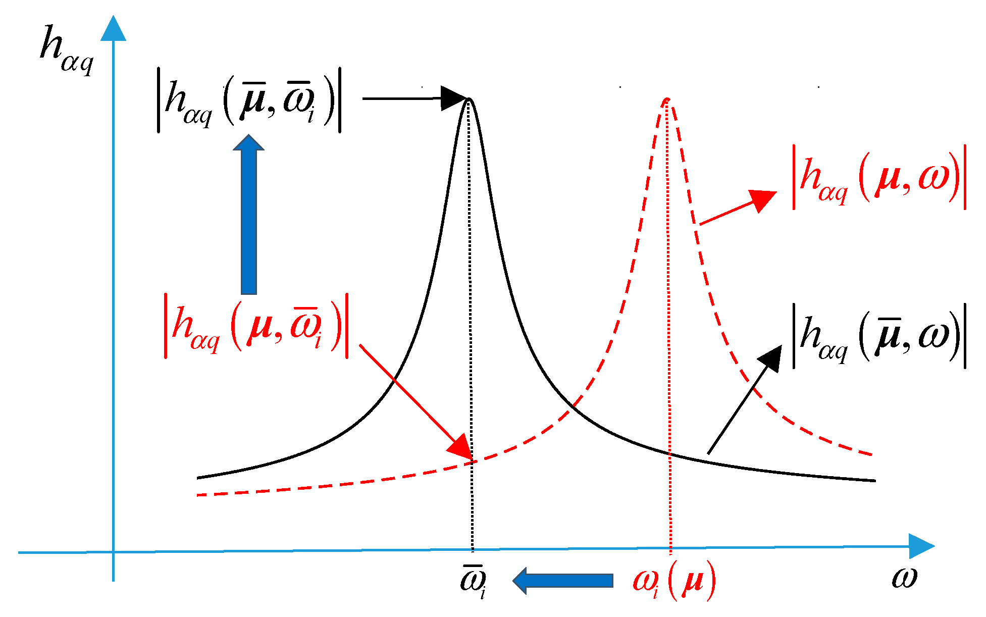
- Involving the natural frequency:It can be seen from Figure 2 that reaches its local maximum value at , and so attains the local minimum value at . Therefore, when the modeled damage factors converge to the actual damage factors, , then the modeled natural frequency converges to the measured natural frequency, , and . In the traditional objective function, the frequency error term also reaches its minimum value when . Therefore, the objective function can be modified by replacing with .
According to these two characteristics, an improved objective function of Equation (5) is proposed. It is obtained by replacing the mode shape and frequency parts of the theoretical FE model with the frequency response, as discussed above.
The frequency response in Equation (5) can be quickly computed using the SVDM, which is described in the next section.
3.2. Substructural Virtual Distortion Method (SVDM) in Frequency Domain
The SVDM [39] can be used to quickly compute the frequency response of the FE model of the damaged structure, without the numerically costly process of the re-analysis of the entire structure. During the optimization, it is applied to calculate the frequency response of the damaged structure (as defined by the modified damage factors) with a high computational efficiency.
Zhang and Jankowski [39] studied the SVDM in detail and deduced the respective formulas. The FRF of the FE model of the damaged structure is equivalently modeled as a superposition of the FRF of the undamaged structure and the frequency responses to certain virtual distortions that model the substructural damages. The frequency response can be computed as shown in Equations (6) and (7):
where is the frequency response of the undamaged structure at the sensor to the unit impulse distortion ; is the j-th actual virtual distortion coefficient of the i-th substructure of the undamaged structure to the unit impulse distortion ; and are the actual distortion coefficient and virtual distortion coefficient of the undamaged structure, respectively [39].
In Equations (6) and (7), and represent the characteristics of the original undamaged structure, and they can be computed in advance under the unit impulse excitation using the theoretical FE model. Therefore, the frequency response of the damaged structure can be computed quickly by first solving Equation (7) for and then substituting the result into Equation (6). Note that the size of Equation (7) is related to the total number of the damage factors (substructures) instead of the total number of all structural DOFs. In this way, the time-consuming structural re-analysis in the traditional approach is avoided.
During the optimization procedure for the purpose of damage identification, the main numerical effort is to calculate for given damage factors, i.e., to solve Equation (7). Therefore, the number of damage factors to be identified and the number of the considered virtual distortions have a large influence on computational efficiency. In order to reduce the number of virtual distortions, only the crucial virtual distortions are considered. They are selected by analyzing the correlation between the actual distortions and the structural frequency response [39].
3.3. Selection of Key Parameters in Improved Objective Function
The calculation of the frequency response in the improved objective function depends on the damping ratio and excitation. The weight of the frequency and mode shape terms of the theoretical FE model in the improved objective function will affect the accuracy of damage identification, and the gradient of the improved objective function will be helpful to increase the optimization efficiency. So, in order to ensure the efficiency of the improved objective function and the accuracy of damage identification results, the selection of these key parameters is very important. The selection principles of these parameters are introduced and discussed as below.
3.3.1. Selection of the Damping Ratio
The frequency response is used to replace the mode shape and natural frequency terms in the traditional objective function of Equation (1). The frequency response depends on the assumed damping ratio of the modeled structure, so that the selection of the damping ratio has a certain impact on the optimization process. When the damping ratio of the model is zero, the extreme point of is exactly in the position of . However, an obvious steep peak will occur in the curve of at the position of , which is not conducive to optimization. On the other hand, when the damping ratio is large, the curve at the extreme point will be relatively gentle, but the peak value may not be in the position of , and it might be affected by other modes. After calculating and comparing the damping ratio of each mode, it has been decided to use the typical value of 0.01.
3.3.2. Selection of Excitation
The frequency response represents the response to the excitation , so that the characteristics of are closely related to the excitation. Since the excitation is applied numerically in the FE model, it can be freely selected. In order to obtain a frequency response that contains more accurate modal information, different excitations can be applied for each natural frequency to be identified. Here, the excitation is chosen for the i-th frequency to be identified, where is the i-th mode shape of the theoretical undamaged FE model. The objective function of Equation (5) can be further improved as shown in Equation (8).
where and represent the structural frequency response obtained by the theoretical FE model under excitation .
3.3.3. Selection of the Weights of the Frequency and Mode Shape Terms
The objective function of Equation (8) includes two parts: the part related to the mode shape and the part related to the natural frequencies, which is as shown in Equation (9). The theoretical range of the mode shape part is the interval [0,1]. The minimum value of the part is zero, while the maximum value is related to the factors such as excitation, structural characteristics and damping. Therefore, the magnitude of the two parts of Equation (9) may vary greatly. In order to ensure their balanced influence on the objective function, the modal shape weight and the frequency weight should be taken reasonably. The trial estimation method is adopted to determine the weights: Firstly, one substructure is selected, indexed by j, as if only the j-th substructure was damaged, and a damage factor is assumed. Then the mode shape part and the frequency part of the objective function can be calculated by Equation (9). Denote the maximum values of and by and , respectively. Finally, the weight coefficients are calculated as , , which is to ensure that the numerical ranges of the two parts are as close as possible.
3.3.4. The Gradient of the Improved Objective Function
The gradient of the objective function might be used to increase the efficiency of optimization. In Equation (8), the first derivative of the FRF with respect to the damage factor can be obtained by differentiation of Equations (6) and (7). Then the gradient expression of the objective function is as shown in Equation (10):
where , , can be calculated by Equation (11).
For the calculation of the gradient of the objective function, it is crucial to find the first derivative of the FRF with respect to the damage factor, i.e., . The first derivative is applied to both sides of Equation (6), and Equation (12) is obtained.
The first derivative with respect to the damage factor is then applied to both sides of Equation (7), which yields Equation (13).
where ; and is Kronecker’s delta:
Equation (13) is a linear equation that can be solved to obtain the first derivative of the substructural virtual distortion with respect to the damage factor. Then, the first derivative of the FRF with respect to the damage factor can be obtained by substituting into Equation (12). In this way, the entire gradient of the objective function can be successively obtained.
3.3.5. Optimization Efficiency
When the traditional objective function is used, the computational efficiency is related to the total number of DOFs of the entire structure. For the improved objective function proposed here, the computational efficiency is related to the number of damage factors to be identified and the number of considered virtual distortions. For large-scale structures with many DOFs, the number of damage factors to be identified is far less than the number of substructural DOFs, so that the optimization efficiency using the improved objective function is relatively high.
This paper mainly focuses on the derivation of the improved objective function and on the verification of the related enhancement of the optimization efficiency. The form of the proposed objective function is independent of the algorithm used to minimize it. Therefore, many optimization methods in MATLAB and other computational software such as fmincon, patternsearch or Genetic Algorithm (GA), can be adopted for optimization. In fact, any optimization method can be used to compare the optimization efficiency using the traditional formulation and the proposed improved objective function. The fmincon optimization toolbox in MATLAB is used to find the minimum of a constrained nonlinear multivariable function in this paper.
4. Numerical Simulation
4.1. The Structural FE Model
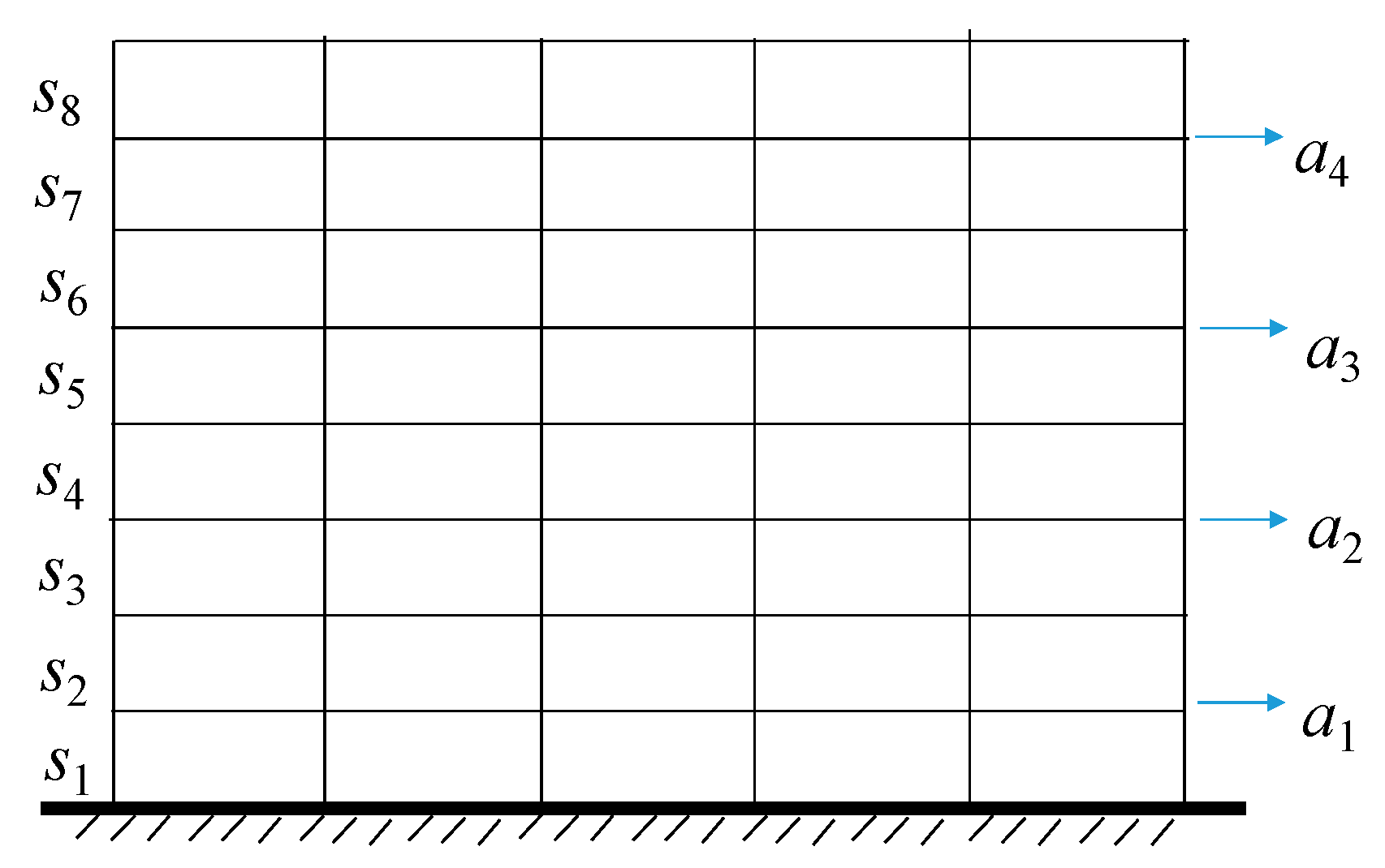
The accuracy of the proposed method is verified by a FE model of an eight-story steel frame structure, as shown in Figure 3. The structural height of each story is 3 m, with a total of five spans, and each span is 5 m. The material density is 7850 kg/m3, and the elastic modulus is 210 GPa. The cross-sectional area of the beam and column is 0.01 m2, and the section moment of inertia is 8.33 × 10⁻⁵ m4. Each beam and column of the structure is a unit, and the structural FE model has 144 DOFs in total. Rayleigh damping is adopted for the structure; the first two orders of damping ratio are both 0.01. The FE model is established using MATLAB.
As shown in Figure 3, six columns and five beams of each story are treated as a substructure, and the substructures are denoted by S1–S8 and counted from the bottom. Considering that only a small part of the structure is usually damaged, two of the eight substructures are assumed to be damaged in this paper. It is assumed that the substructures S2 and S5 are damaged with the damage factors of 0.6 and 0.7, respectively. In order to verify the validity of the proposed method, all eight damage factors are optimized for identification. If the identified damage factor of the substructure is less than 1, the damage of the substructure can be recognized; if the damage factor is equal to 1, the substructure is undamaged.
4.2. Substructure Response
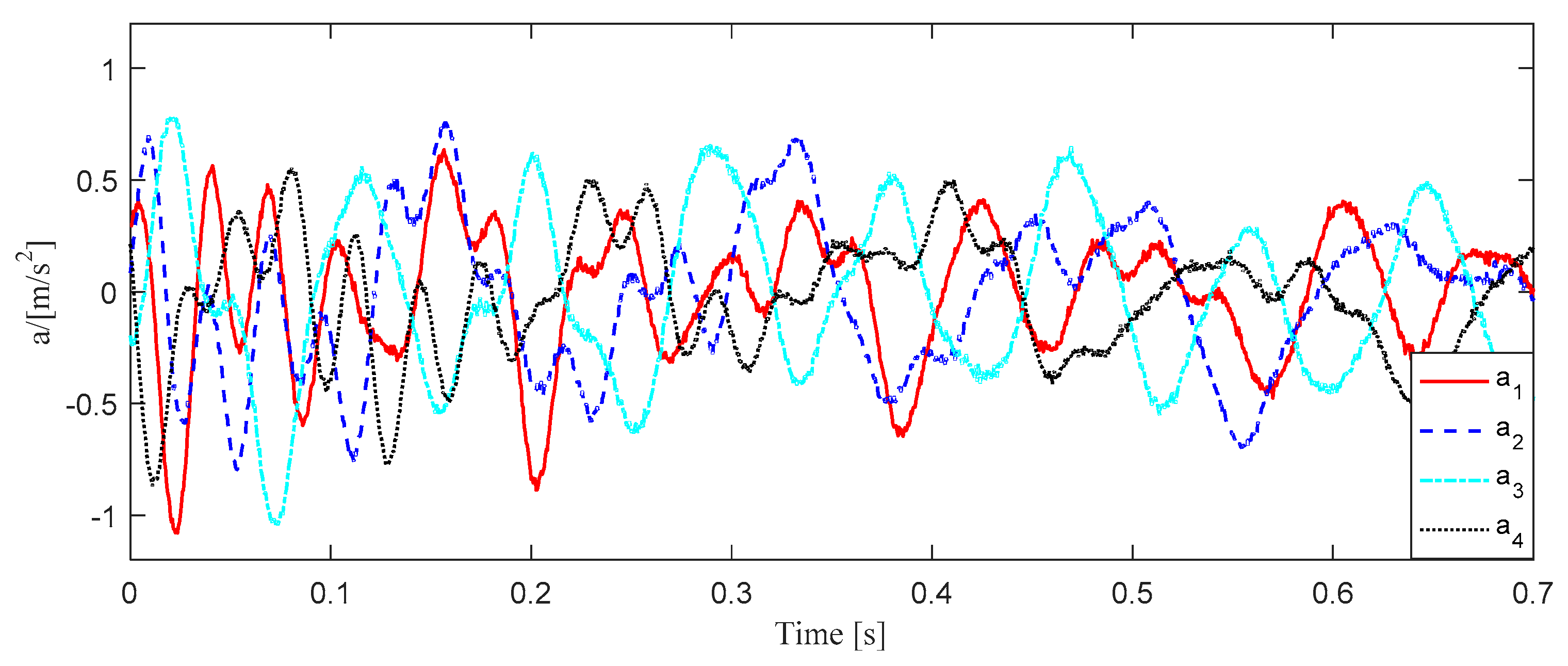
Acceleration sensors are arranged on the beams of substructures S1, S3, S5, and S7, respectively, to measure the horizontal acceleration of the structure. The sampling frequency is 200 Hz with a total sampling time of 0.7 s. Given the initial state of the randomly damaged structure, the free response of the structure is calculated by the Newmark integration method with the influence of 5% Gaussian noise. The response of sensors is shown in Figure 4.
4.3. Structural Mode Shapes and Frequencies
The first six mode shapes and frequencies of the theoretical undamaged structural model are shown in Figure 5 and Table 1 respectively. The first six modes of the damaged structure are identified by the eigen realization algorithm (ERA) using the structural free response in Figure 4. Comparing the frequency identified by the ERA of the damaged structure (column “Identified” in Table 1) with the frequency calculated by the FE model of damaged structure (“Damaged model” in Table 1), the results are very close, indicating that the recognition result is robust to noise. In fact, the error of the high-order mode shape identified is relatively larger, so the first six natural frequencies and the first three mode shapes identified are selected as the basis for damage identification in this numerical simulation. The discussion about the number of modes used can be found in Section 4.7, together with an example damage identification performed using fewer modes in order to verify the influence of the number of modes on the accuracy of damage identification results.
4.4. Selection of the Main Virtual Distortions
In the process of damage identification, the main virtual distortion of each substructure is analyzed and selected at first [39]. Using the FE model of the undamaged structure, the stiffness matrix of each substructure is assembled, and its eigenvalue decomposition is carried out. Then the positive eigenvalues, i.e., the number of virtual distortions are shown in Table 2, which is 261 virtual distortions in total. If all virtual distortions are used, a 261 × 261 linear system of equations should be calculated to determine one virtual distortion when solving Equation (7). In order to reduce the computational cost, the correlation between the virtual distortions of each substructure and the distortion of the undamaged structure is analyzed. Finally, the correlations are sorted from large to small and cumulatively summed, and those virtual distortions are retained and further considered in computations, for which the accumulated correlation is below 99%. The main virtual distortions for the first six natural frequencies identified are shown in Table 2.
The number of selected virtual distortions is about 20% of the total number under each frequency, which effectively reduces the computational complexity of solving the linear Equation (7). It has an even more significant advantage in the application to large complex structures.
4.5. Fast Calculation of Structural Frequency Response
Firstly, the FRF of the undamaged structure is calculated according to the theoretical FE model. And the FRF of the first six frequencies of the damaged structure corresponding to the position of four measuring points is calculated respectively, where the amplitude of excitation used here is related to each mode shape of the undamaged structural model as explained in Section 3.3.2. Then, the virtual distortion of the associated substructure can be calculated by Equation (7). Finally, the FRF of the damaged structure can be obtained by Equation (6). The calculation process of of the damaged structure corresponding to the 1st natural frequency is taken as an example to describe the above process introduced.
Given the damage factor , the 1st mode shape of the theoretical undamaged model is applied as a pulse excitation to the undamaged structure, and the frequency responses in Equations (6) and (7) can be calculated. Then, the virtual distortion of the substructure can be obtained by solving Equation (7), where the number of main virtual distortions is 48, i.e., the dimensions of the linear equations are 48 × 48. Finally, the FRF of the damaged structure with damage factor is quickly calculated by Equation (6).
When the real damage factor is given, the amplitudes obtained by SVDM at the four measuring points of the damaged structure are ; the amplitudes obtained by the structural modes at the four measuring points of the damaged FE model are . The results obtained by the two methods are very close, which shows the accuracy of the structural frequency response constructed by SVDM.
4.6. Damage Identification Based on the Proposed Method
The basic damage scenario described above is that the substructures S2 and S5 are damaged with the damage factors 0.6 and 0.7. The respective damage identification results are presented as damage case 1. Additionally, in order to verify the applicability of the proposed method, damage identification under further multiple damage cases is carried out and discussed in the following.
4.6.1. Damage Case 1
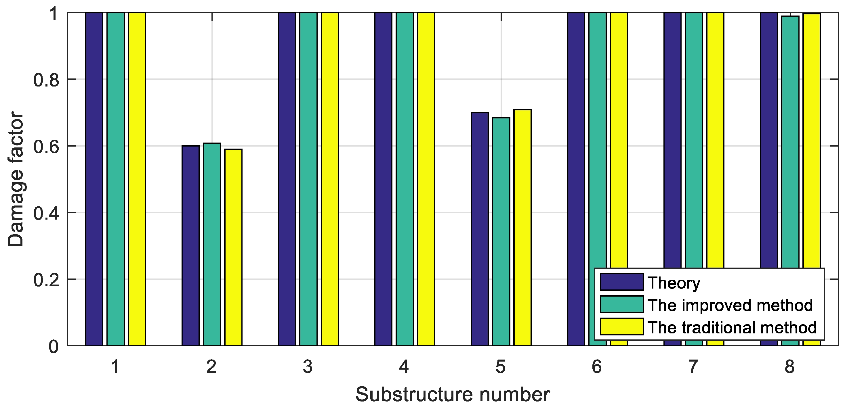
In the optimization process, the initial value of the damage factor (usually , i.e., the undamaged state) is first selected. After calculating the value range of the objective function of mode shape and frequency respectively, the weight coefficients of mode shape and frequency in optimization are estimated: . Then, the damage factor is updated iteratively using the fmincon optimization toolbox in MATLAB until the objective function reaches its minimum value. The gradient of the objective function, as derived in Section 3.3.4, is included for faster or more reliable computations. The identification results of damage factors are shown in Figure 6 and Table 3. It can be seen from Table 3 that the results identified using the improved and traditional objective function are both close to the theoretical values, and the error is less than 0.03, which meets the requirements of damage identification. The improved objective function proposed contains the measured modes of actual damaged structures and the FRF constructed by the theoretical FE model using the SVDM. The damage identification method based on the frequencies and mode shapes has been validated in numerical and experimental investigation and the references are given in the introduction. The SVDM utilized in the improved method has also been verified by experimental research in Reference [39]. In the simulation, the accuracy of the improved method is proved to be consistent with the traditional method by the theoretical research, so the effectiveness of the improved method is verified and confirmed.
Moreover, the computational efficiency is discussed. In the numerical simulation, there are 144 DOFs of the FE model. When the traditional objective function is adopted, all DOFs should be calculated to obtain the structural modes, so the computational cost is of the order of O(1443). However, the number of damage factors to be identified is eight, and the number of main virtual distortions is about 50. So the computational cost based on the improved objective function is of the order of O(6 × 503), which shows that the proposed method using an improved objective function is more efficient. In practical calculation, the time of optimization is about 0.83 s by using the improved objective function, while by using the traditional objective function the time of optimization is about 2.73 s. As a result, the computational efficiency is increased approximately three times using the method proposed in this numerical simulation.
4.6.2. Damage Case 2
In damage case 1, two large damages are considered, and the results are relatively accurate. In damage case 2, multiple smaller damages are considered, and the damage identification results are shown in Table 4. It can be seen from Table 4 that the results identified using the improved and traditional objective function are very close, which verifies the accuracy of the proposed method. Besides, they are both close to the theoretical values and the error is less than 0.03, which meets the requirements of damage identification. Therefore, the accuracy and validity of the proposed method are verified also in the case of multiple smaller damages.
4.6.3. Damage Case 3
In damage case 3, a single smaller damage is considered. The damage identification results are shown in Table 5. It can be seen from Table 5 that the results identified using the improved and traditional objective function are very close, which verifies the accuracy of the proposed method. Besides, they are both close to the theoretical values and the error is less than 0.03, which meets the requirements of damage identification. Therefore, the accuracy and validity of the proposed method are verified also in the case of a single smaller damage.
4.6.4. Damage Case 4
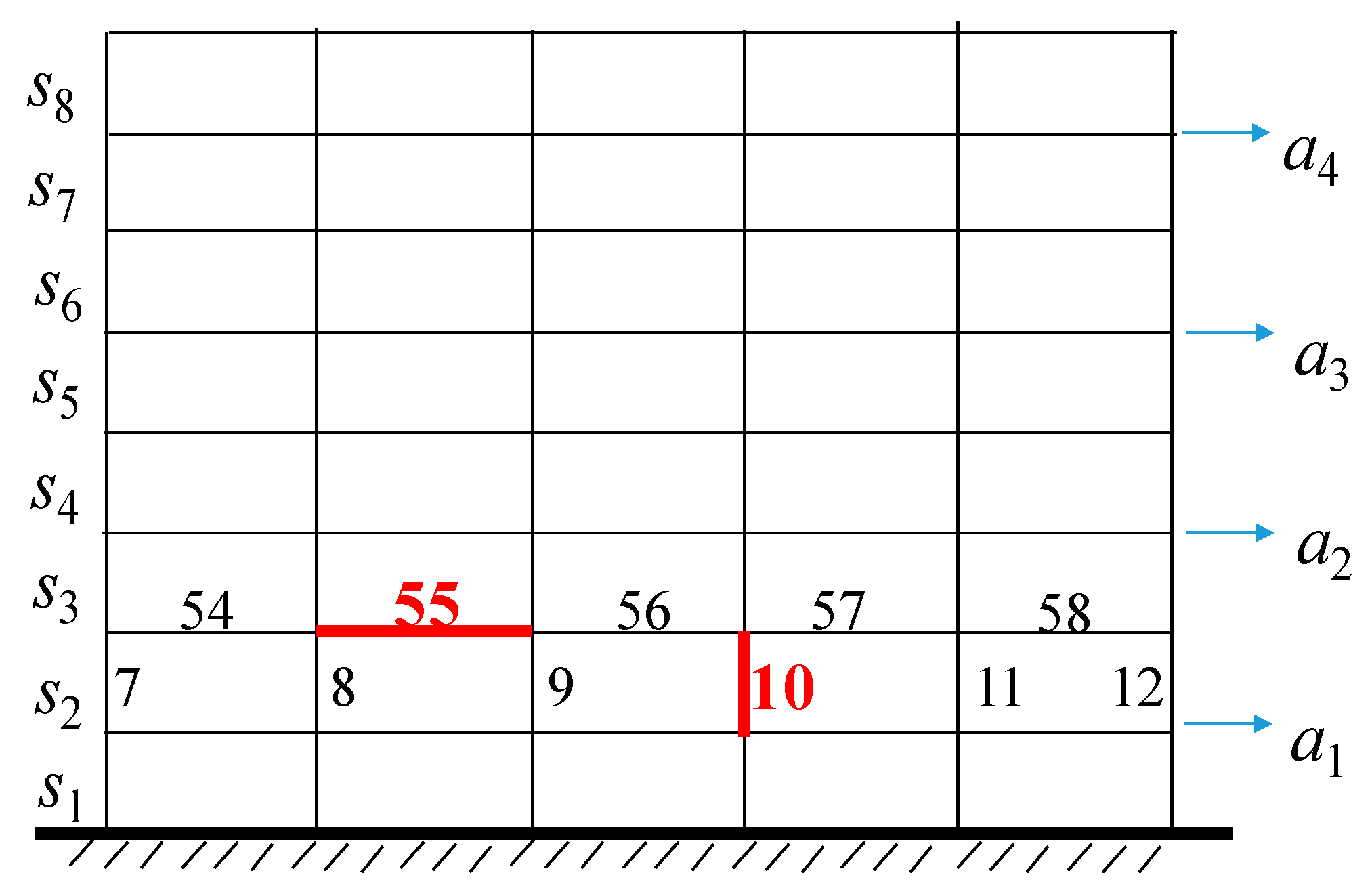
In damage case 4, the damage of a single beam or column is studied. The beams and columns in the model are numbered for ease of illustration. For columns, they are numbered from left to right and then from bottom to top. A total of 48 columns are numbered 1–48. Then the beams are consecutively numbered in accordance with the same rule. There are 40 beams numbered 49–88.
The damage of a single beam or column is studied under four separate damage cases, which are shown in Table 6: The 10th column with a damage factor of 0.5 and 0.8; and the 55th beam with a damage factor of 0.5 and 0.8. The 10th column and the 55th beam belong to the 2nd substructure, as shown in Figure 7. Under the above four damage cases, the numerical simulation is carried out and the damage of eight substructures is identified. The damage factors of other substructures are close to the theoretical value of 1, so only the results of the second substructure are listed in Table 6.
As shown in Table 6, when the damage factor of the 10th column is 0.5, it can be detected that the 2nd substructure has been damaged. However, it is difficult to detect the structural damage when the damage factor is smaller than 0.8. Compared with columns, the contribution of beams to structural lateral stiffness is smaller, so the damage is more difficult to detect under the same damage factor.
When the damage factor of the 10th column is 0.5, it can be detected that the 2nd substructure has been damaged. In order to further identify damage, each of the beams and columns is treated as a separate substructure. Therefore, there are 11 substructures and 11 damage factors to be identified in the second floor. The damage identification results are shown in Table 7. From Table 7, it can be roughly judged that a column has been damaged, but it is almost impossible to identify which column has been damaged. It is because the identification used the structural frequency and mode shape, which conveys global information about the structure and are insensitive to local damage. If local damage is to be identified, a method suitable for local damage identification should be used. Such a method has been proposed by the author and it can be found in Reference [29] that is referenced in the introduction.
When the eleven substructures of the second floor are to be identified using the first three mode shapes and first six natural frequencies, the time of optimization is about 0.43 s using the improved objective function, while it is about 20.96 s using the traditional objective function. The number of the damage factors (optimization parameters) is increased by three, which is from 8 to 11. When using the traditional objective function, the total time of optimization is accordingly increased to a significant degree. However, when using the improved objective function, the column or beam substructure is much simpler than the previous floor substructure, so the number of the selected virtual distortions is reduced by the SVDM from about 50 to about 12, and the time is reduced from 0.83 s to 0.43 s. This illustrates the high efficiency of the proposed method.
4.7. The Discussion about the Number of Modes Used
In this paper, the first six frequencies and first three mode shapes are adopted to identify the damage. The influence of the number of the considered modes on the damage identification results has been verified by performing identification based on fewer natural frequencies and mode shapes. The maximum differences between the identified damage factor and the theoretical value using different numbers of modes and the improved and traditional method are shown in Table 8 and Table 9, respectively.
It can be seen from Table 8 and Table 9 that the identification errors obviously increase when the number of the considered modes decreases. Especially, if only the first mode shape was used, there would be an obvious misjudgment, which indicates the information is insufficient.
In practice, modal information is obtained from measurements always with a certain error. The error of higher mode shapes and frequencies is larger, so the first six frequencies and the first three mode shapes are selected in this paper. In order to ensure the accuracy of damage identification, there must be enough modal information. From the numerical simulation results in Table 8 and Table 9, one can infer that the selection of the first six frequencies and the first three mode shapes is sufficient, which indicates that the selection in this paper is reasonable.
5. Conclusions
In order to avoid repeated calculation of structural modes and to improve the optimization efficiency, an improved objective function for damage identification based on the SVDM is proposed. A numerical model of an eight-story frame structure is used to verify the effectiveness of the proposed method. The main conclusions are as follows:
- Considering the characteristic that the amplitude of the frequency response attains a local maximum at the position of structural natural frequencies, an improved objective function is developed which avoids the repeated calculation of structural modes in the optimization procedure and improves the computational efficiency.
- Utilizing the fast structural re-analysis approach of the SVDM, frequency response in the improved objective function can be computed quickly, and the gradient expression of the objective function can be derived which further improves the optimization efficiency.
- The optimization efficiency using the traditional objective function is related to the number of DOFs of the entire structure, while the optimization efficiency based on the improved objective function is related to the number of damage factors to be identified and the number of selected virtual distortions.
Author Contributions
Conceptualization, J.H., Q.Z. and Ł.J.; methodology, J.H. and Q.Z.; software, S.W. and J.H.; validation, S.W. and J.H.; data curation, S.W.; writing—original draft preparation, S.W.; writing—review and editing, S.W. and J.H., Q.Z. and Ł.J.; supervision, J.H.
Funding
This research was funded by National Key Research and Development Program of China (2018YFC0705604), National Natural Science Foundation of China (NSFC) (51878118), Liaoning Provincial Natural Science Foundation of China (20180551205), Key Laboratory of Structures Dynamic Behavior and Control (Ministry of Education) in Harbin Institute of Technology of China (HITCE201707) and the project DEC- 2017/25/B/ST8/01800 of the National Science Centre, Poland.
Conflicts of Interest
The authors declare no conflict of interest.
References
- Annamdas, V.G.M.; Bhalla, S.; Soh, C.K. Applications of structural health monitoring technology in Asia. Struct. Health Monit. 2017, 16, 324–346. [Google Scholar] [CrossRef]
- Zhou, L.R.; Yan, G.R.; Wang, L.; Ou, J.P. Review of benchmark studies and guidelines for structural health monitoring. Adv. Struct. Eng. 2013, 16, 1187–1206. [Google Scholar] [CrossRef]
- Xie, L.Y.; Zhou, Z.W.; Zhao, L.; Wan, C.F.; Tang, H.S.; Xue, S.T. Parameter identification for structural health monitoring with extended Kalman filter considering integration and noise effect. Appl. Sci. 2018, 8, 2480. [Google Scholar] [CrossRef]
- Hu, W.H.; Tang, D.H.; Teng, J.; Said, S.; Rohrmann, R.G. Structural health monitoring of a prestressed concrete bridge based on statistical pattern recognition of continuous dynamic measurements over 14 years. Sensors 2018, 18, 4117. [Google Scholar] [CrossRef] [PubMed]
- Jiang, T.Y.; Zhang, Y.W.; Wang, L.; Zhang, L.; Song, G.B. Monitoring fatigue damage of modular bridge expansion joints using piezoceramic transducers. Sensors 2018, 18, 3973. [Google Scholar] [CrossRef] [PubMed]
- Shen, S.; Jiang, S.F. Distributed deformation monitoring for a single-cell box girder based on distributed long-gage fiber bragg grating sensors. Sensors 2018, 18, 2597. [Google Scholar] [CrossRef] [PubMed]
- Na, W.S.; Seo, D.W.; Kim, B.C.; Park, K.T. Effects of applying different resonance amplitude on the performance of the impedance-based health monitoring technique subjected to damage. Sensors 2018, 18, 2267. [Google Scholar] [CrossRef] [PubMed]
- Fan, W.; Qiao, P.Z. Vibration-based damage identification methods: A review and comparative study. Struct. Health Monit. 2011, 10, 83–111. [Google Scholar] [CrossRef]
- Xu, K.; Deng, Q.S.; Cai, L.J.; Ho, S.C.; Song, G.B. Damage detection of a concrete column subject to blast loads using embedded piezoceramic transducers. Sensors 2018, 18, 1377. [Google Scholar] [CrossRef] [PubMed]
- Zhao, Y.; Noori, M.; Altabey, W.A.; Ghiasi, R.; Wu, Z.S. Deep learning-based damage, load and support identification for a composite pipeline by extracting modal macro strains from dynamic excitations. Appl. Sci. 2018, 8, 2564. [Google Scholar] [CrossRef]
- Moreno-Gomez, A.; Amezquita-Sanchez, J.P.; Valtierra-Rodriguez, M.; Perez-Ramirez, C.A.; Dominguez-Gonzalez, A.; Chavez-Alegria, O. Emd-Shannon entropy-based methodology to detect incipient damages in a truss structure. Appl. Sci. 2018, 8, 2068. [Google Scholar] [CrossRef]
- Kordestani, H.; Xiang, Y.Q.; Ye, X.W.; Jia, Y.K. Application of the random decrement technique in damage detection under moving load. Appl. Sci. 2018, 8, 753. [Google Scholar] [CrossRef]
- Peng, J.; Hu, S.; Zhang, J.; Cai, C.S.; Li, L.Y. Influence of cracks on chloride diffusivity in concrete: A five-phase mesoscale model approach. Constr. Build. Mater. 2019, 197, 587–596. [Google Scholar] [CrossRef]
- Hearn, G.; Testa, R.B. Modal analysis for damage detection in structures. J. Struct. Eng. 1991, 117, 3042–3063. [Google Scholar] [CrossRef]
- Dilena, M.; Morassi, A. The use of antiresonances for crack detection in beams. J. Sound Vib. 2004, 276, 195–214. [Google Scholar] [CrossRef]
- Shi, Z.Y.; Law, S.S.; Zhang, L.M. Damage localization by directly using incomplete mode shapes. J. Eng. Mech. 2000, 126, 656–660. [Google Scholar] [CrossRef]
- Pandey, A.K.; Biswas, M.; Samman, M.M. Damage detection from changes in curvature mode shapes. J. Sound Vib. 1991, 145, 321–332. [Google Scholar] [CrossRef]
- Shi, Z.Y.; Law, S.S.; Zhang, L.M. Structural damage localization from modal strain energy change. J. Sound Vib. 1998, 218, 825–844. [Google Scholar] [CrossRef]
- Kim, J.T.; Ryu, Y.S.; Cho, H.M.; Stubbs, N. Damage identification in beam-type structures: Frequency-based method vs mode-shape-based method. Eng. Struct. 2003, 25, 57–67. [Google Scholar] [CrossRef]
- Huynh, T.C.; Lee, S.Y.; Dang, N.L.; Kim, J.T. Vibration-based structural identification of caisson-foundation system via in situ measurement and simplified model. Struct. Control Health Monit. 2019, 26, e2315. [Google Scholar] [CrossRef]
- Wang, J.Y.; Ko, J.M.; Ni, Y.Q. Modal sensitivity analysis of Tsing Ma Bridge for structural damage detection. Proc. SPIE Int. Soc. Opt. Eng. 2000, 3995, 300–311. [Google Scholar]
- Guo, H.Y.; Li, Z.L. Structural multi-damage identification based on modal strain energy equivalence index method. Int. J. Struct. Stab. Dyn. 2014, 14, 1450028. [Google Scholar] [CrossRef]
- Kaveh, A.; Maniat, M. Damage detection based on MCSS and PSO using modal data. Smart Struct. Syst. 2015, 15, 1253–1270. [Google Scholar] [CrossRef]
- Cui, H.Y.; Xu, X.; Peng, W.Q.; Zhou, Z.H.; Hong, M. A damage detection method based on strain modes for structures under ambient excitation. Measurement 2018, 125, 438–446. [Google Scholar] [CrossRef]
- Liang, Y.B.; Li, D.S.; Song, G.B.; Feng, Q. Frequency Co-integration-based damage detection for bridges under the influence of environmental temperature variation. Measurement 2018, 125, 163–175. [Google Scholar] [CrossRef]
- Qin, S.Q.; Zhang, Y.Z.; Zhou, Y.L.; Kang, J.T. Dynamic model updating for bridge structures using the Kriging model and PSO algorithm ensemble with higher vibration modes. Sensors 2018, 18, 1879. [Google Scholar] [CrossRef] [PubMed]
- Gao, H.Y.; Guo, X.L.; Hu, X.F. Crack identification based on Kriging surrogate model. Struct. Eng. Mech. 2012, 41, 25–41. [Google Scholar] [CrossRef]
- Guo, J.L.; Ma, L.Y.; Li, Y.J. A new structural damage identification method based on Kriging surrogate model. China Mech. Eng. 2016, 27, 1203–1207. [Google Scholar]
- Hou, J.L.; An, Y.H.; Wang, S.J.; Wang, Z.Z.; Jankowski, Ł.; Ou, J.P. Structural damage localization and quantification based on additional virtual masses and Bayesian theory. J. Eng. Mech. 2018, 144, 04018097. [Google Scholar] [CrossRef]
- Kołakowski, P.; Wikło, M.; Holnicki-Szulc, J. The virtual distortion method-a versatile reanalysis tool for structures and systems. Struct. Multidiscip. Optim. 2008, 36, 217–234. [Google Scholar] [CrossRef]
- Świercz, A.; Kołakowski, P.; Holnicki-Szulc, J. Damage identification in skeletal structures using the virtual distortion method in frequency domain. Mech. Syst. Signal Process. 2008, 22, 1826–1839. [Google Scholar] [CrossRef] [Green Version]
- Zhang, Q.X.; Jankowski, Ł.; Duan, Z.D. Simultaneous identification of moving masses and structural damage. Struct. Multidiscip. Optim. 2010, 42, 907–922. [Google Scholar] [CrossRef] [Green Version]
- Xing, Z.H.; Mita, A. A substructure approach to local damage detection of shear structure. Struct. Control Health Monit. 2012, 19, 309–318. [Google Scholar] [CrossRef]
- Li, J.; Law, S.S.; Ding, Y. Substructure damage identification based on response reconstruction in frequency domain and model updating. Eng. Struct. 2012, 41, 270–284. [Google Scholar] [CrossRef]
- Hou, J.L.; Jankowski, Ł.; Ou, J.P. Experimental study of the substructure isolation method for local health monitoring. Struct. Control Health Monit. 2012, 19, 491–510. [Google Scholar] [CrossRef]
- Zhu, H.P.; Mao, L.; Weng, S. Calculation of dynamic response sensitivity to substructural damage identification under moving load. Adv. Struct. Eng. 2013, 16, 1621–1632. [Google Scholar] [CrossRef]
- Li, J.; Hao, H. Substructure damage identification based on wavelet-domain response reconstruction. Struct. Health Monit. 2014, 13, 389–405. [Google Scholar] [CrossRef]
- Hou, J.L.; Jankowski, Ł.; Ou, J.P. Frequency-domain substructure isolation for local damage identification. Adv. Struct. Eng. 2015, 18, 137–153. [Google Scholar] [CrossRef]
- Zhang, Q.X.; Jankowski, Ł. Damage identification using structural modes based on substructure virtual distortion method. Adv. Struct. Eng. 2017, 20, 257–271. [Google Scholar] [CrossRef]
Figure 1.
Summation of modal contributions into the frequency response.
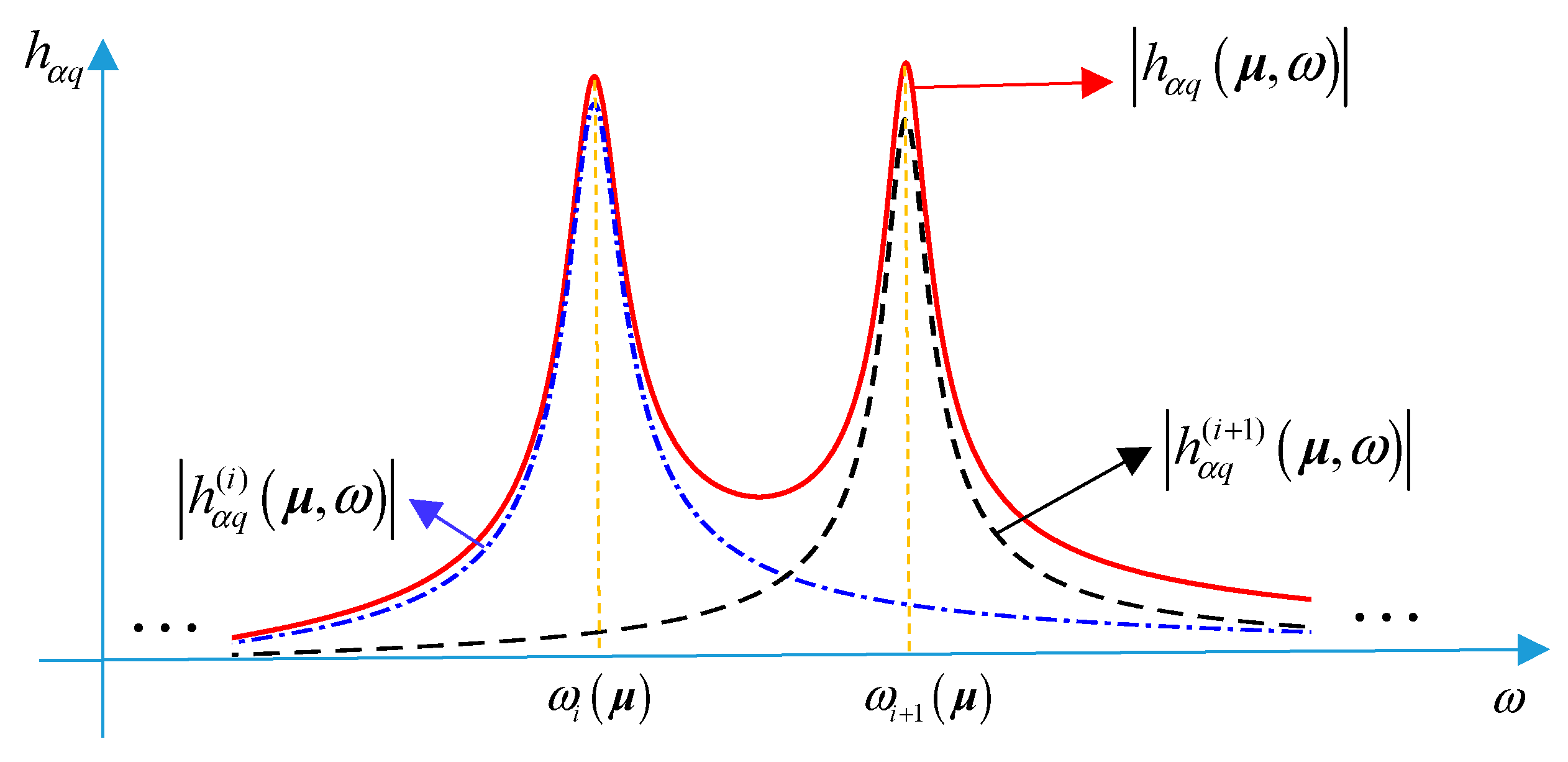
Figure 2.
The frequency response of the damaged structure.

Figure 3.
An eight-story steel frame structure model.

Figure 4.
The simulated structural response of sensors

Figure 5.
The first six mode shapes of the theoretical undamaged model.
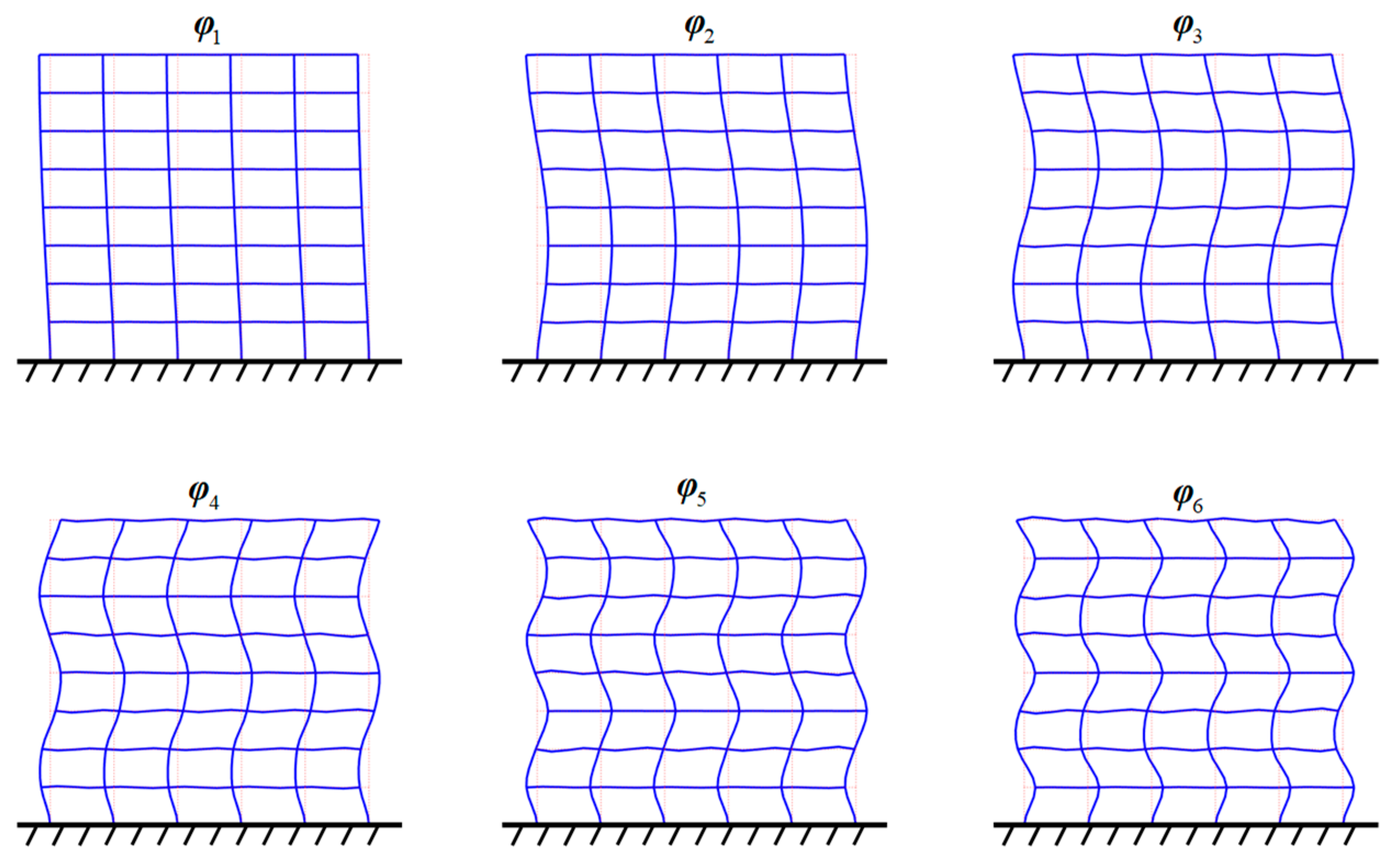
Figure 6.
The identified damage extent.

Figure 7.
The location of 10th column and the 55th beam.

Table 1.
The first six frequencies of structure in different cases (Hz).
| Order | Identified | Damaged Model | Undamaged Model |
|---|---|---|---|
| 1 | 1.972 | 1.961 | 2.133 |
| 2 | 6.141 | 6.142 | 6.568 |
| 3 | 11.254 | 11.257 | 11.472 |
| 4 | 16.091 | 16.095 | 16.963 |
| 5 | 22.007 | 22.006 | 23.052 |
| 6 | 27.330 | 27.339 | 29.484 |
Table 2.
The number of main virtual distortions corresponding to the first six frequencies of each substructure.
Table 2.
The number of main virtual distortions corresponding to the first six frequencies of each substructure.
| Number | All | ω1 | ω2 | ω3 | ω4 | ω5 | ω6 |
|---|---|---|---|---|---|---|---|
| 1 | 18 | 2 | 1 | 0 | 2 | 3 | 3 |
| 2 | 35 | 8 | 8 | 7 | 3 | 6 | 7 |
| 3 | 34 | 7 | 10 | 5 | 8 | 7 | 3 |
| 4 | 35 | 6 | 7 | 7 | 7 | 6 | 7 |
| 5 | 34 | 6 | 7 | 8 | 6 | 8 | 7 |
| 6 | 35 | 5 | 6 | 5 | 7 | 7 | 3 |
| 7 | 34 | 8 | 9 | 4 | 9 | 10 | 17 |
| 8 | 36 | 6 | 5 | 6 | 7 | 7 | 7 |
| Total | 261 | 48 | 53 | 42 | 49 | 54 | 54 |
Table 3.
Comparison of damage identification results using the improved objective function and traditional objective function.
Table 3.
Comparison of damage identification results using the improved objective function and traditional objective function.
| No | Theory | The Improved Method | The Traditional Method |
|---|---|---|---|
| 1 | 1.0000 | 0.9999 | 0.9996 |
| 2 | 0.6000 | 0.6084 | 0.5897 |
| 3 | 1.0000 | 0.9999 | 1.0000 |
| 4 | 1.0000 | 0.9998 | 0.9997 |
| 5 | 0.7000 | 0.6846 | 0.7087 |
| 6 | 1.0000 | 0.9998 | 1.0000 |
| 7 | 1.0000 | 0.9997 | 1.0000 |
| 8 | 1.0000 | 0.9896 | 0.9963 |
Table 4.
Damage identification results with multiple smaller damages.
| No | Theory | The Improved Method | The Traditional Method |
|---|---|---|---|
| 1 | 1.0000 | 0.9999 | 1.0000 |
| 2 | 0.9000 | 0.8836 | 0.8926 |
| 3 | 1.0000 | 0.9767 | 0.9933 |
| 4 | 0.9000 | 0.9042 | 0.8897 |
| 5 | 0.9400 | 0.9376 | 0.9339 |
| 6 | 1.0000 | 0.9999 | 0.9952 |
| 7 | 0.9600 | 0.9754 | 0.9752 |
| 8 | 1.0000 | 1.0000 | 0.9998 |
Table 5.
Damage identification results with a single smaller damage.
| No | Theory | The Improved Method | The Traditional Method |
|---|---|---|---|
| 1 | 1.0000 | 1.0000 | 1.0000 |
| 2 | 1.0000 | 0.9999 | 1.0000 |
| 3 | 1.0000 | 1.0000 | 1.0000 |
| 4 | 1.0000 | 1.0000 | 1.0000 |
| 5 | 1.0000 | 0.9998 | 1.0000 |
| 6 | 1.0000 | 1.0000 | 1.0000 |
| 7 | 0.9600 | 0.9633 | 0.9653 |
| 8 | 1.0000 | 0.9911 | 0.9900 |
Table 6.
Damage identification results of 2nd substructure with single column/beam damage.
| Damage Case | 10th Column with Damage Factor 0.5 | 10th Column with Damage Factor 0.8 | 55th Beam with Damage Factor 0.5 | 55th Beam with Damage Factor 0.8 |
|---|---|---|---|---|
| The improved method | 0.9205 | 0.9802 | 0.9642 | 0.9908 |
| The traditional method | 0.9246 | 0.9824 | 0.9538 | 0.9875 |
Table 7.
Damage identification results with 11 damage factors of 2nd floor.
| No | Theory | The Improved Method | The Traditional Method | |
|---|---|---|---|---|
| Column | 7 | 1.0000 | 0.7586 | 0.9992 |
| 8 | 1.0000 | 0.7669 | 0.9988 | |
| 9 | 1.0000 | 0.8834 | 0.9980 | |
| 10 | 0.5000 | 0.9319 | 0.9964 | |
| 11 | 1.0000 | 0.9388 | 0.8254 | |
| 12 | 1.0000 | 0.9564 | 0.5761 | |
| Beam | 54 | 1.0000 | 0.9909 | 0.9982 |
| 55 | 1.0000 | 0.9931 | 0.9999 | |
| 56 | 1.0000 | 0.9960 | 0.9998 | |
| 57 | 1.0000 | 0.9967 | 0.9998 | |
| 58 | 1.0000 | 0.9970 | 0.9999 |
Table 8.
Maximum difference between the identified damage factor and the theoretical value in the improved method using different modes.
Table 8.
Maximum difference between the identified damage factor and the theoretical value in the improved method using different modes.
| The First Three Mode Shapes Used | The First Two Mode Shapes Used | The First Mode Shape Used | |
|---|---|---|---|
| The First Six Frequencies Used | 0.0154 | 0.0184 | 0.0365 |
| The First Three Frequencies Used | 0.0320 | 0.0383 | 0.2147 |
Table 9.
Maximum difference between the identified damage factor and the theoretical value in the traditional method using different modes.
Table 9.
Maximum difference between the identified damage factor and the theoretical value in the traditional method using different modes.
| The First Three Mode Shapes Used | The First Two Mode Shapes Used | The First Mode Shape Used | |
|---|---|---|---|
| The First Six Frequencies Used | 0.0103 | 0.0162 | 0.0421 |
| The First Three Frequencies Used | 0.0172 | 0.0206 | 0.1755 |
© 2019 by the authors. Licensee MDPI, Basel, Switzerland. This article is an open access article distributed under the terms and conditions of the Creative Commons Attribution (CC BY) license (http://creativecommons.org/licenses/by/4.0/).
Share and Cite
MDPI and ACS Style
Hou, J.; Wang, S.; Zhang, Q.; Jankowski, Ł. An Improved Objective Function for Modal-Based Damage Identification Using Substructural Virtual Distortion Method. Appl. Sci. 2019, 9, 971. https://doi.org/10.3390/app9050971
AMA Style
Hou J, Wang S, Zhang Q, Jankowski Ł. An Improved Objective Function for Modal-Based Damage Identification Using Substructural Virtual Distortion Method. Applied Sciences. 2019; 9(5):971. https://doi.org/10.3390/app9050971
Chicago/Turabian StyleHou, Jilin, Sijie Wang, Qingxia Zhang, and Łukasz Jankowski. 2019. "An Improved Objective Function for Modal-Based Damage Identification Using Substructural Virtual Distortion Method" Applied Sciences 9, no. 5: 971. https://doi.org/10.3390/app9050971
Note that from the first issue of 2016, this journal uses article numbers instead of page numbers. See further details here.