False Positive RFID Detection Using Classification Models

Abstract

Radio frequency identification (RFID) is an automated identification technology that can be utilized to monitor product movements within a supply chain in real-time. However, one problem that occurs during RFID data capturing is false positives (i.e., tags that are accidentally detected by the reader but not of interest to the business process). This paper investigates using machine learning algorithms to filter false positives. Raw RFID data were collected based on various tagged product movements, and statistical features were extracted from the received signal strength derived from the raw RFID data. Abnormal RFID data or outliers may arise in real cases. Therefore, we utilized outlier detection models to remove outlier data. The experiment results showed that machine learning-based models successfully classified RFID readings with high accuracy, and integrating outlier detection with machine learning models improved classification accuracy. We demonstrated the proposed classification model could be applied to real-time monitoring, ensuring false positives were filtered and hence not stored in the database. The proposed model is expected to improve warehouse management systems by monitoring delivered products to other supply chain partners.

1. Introduction

The Industry 4.0 concept opens opportunities to digitize industrial machines, processes, and assets; providing new insights and efficiently countering various current challenges [1]. Radio frequency identification (RFID) is a key Industry 4.0 enabling technology, and has been widely used throughout manufacturing and supply chains. RFID transfers data between readers and movable tagged objects and has been applied to many diverse areas, including tracking and managing assets in healthcare [2,3,4], reducing misplaced inventory throughout supply chains [5], measuring soil erosion [6], and improving just-in-time operation for automotive logistics [7]. The technology has also provided significant advantages for bee monitoring [8], tracking ship pipes [9], customer purchase behavior analysis [10], inventory management [11], indoor robot patrol [12], etc.

For warehouse management systems (WMSs), RFID can monitor tagged products moving through a gate and subsequently loaded for delivery to other supply chain partners. However, RFID cannot distinguish tagged products that move through the gate or those that enter the reading range accidentally. Tags within reader range but not moved through the gate are called false positive, whereas tagged products moved through the gate and loaded are called true positive readings. These accidental reads occur when the range of the antenna might be extended by metallic objects. Consequently, tags assumed to be clearly out of range can be unexpectedly read by the reader. In addition, false positives can also be due to the tags that are located within the nominal read range but are read accidentally. Since WMSs should correctly calculate the total amount of tagged products loaded, detecting and filtering false positives is critical to ensure the correct delivered product records are retained.

Received signal strength (RSS) is the relative quality of a received signal for a device, which is related to the distance between the tags and antenna for RFID, and has been previously utilized for indoor localization systems (ILSs) [13,14,15,16], indoor mapping and navigation in retail stores [17], indoor tracking system for elderly [18], and gesture recognition [19]. Previous studies confirm RSS approaches to be suitable to detect false positives [20,21,22], where static and moved tags were classified as false positive and true positive readings, respectively. Machine learning models have also been utilized to successfully detect false positives using RSS based features as inputs. However, some retail store-based studies showed that tag movement close to the gate and through the gate were classified as false positive and true positive readings, respectively [23,24]. Therefore, false positive classification must consider other tag movement types, such as tag movement close to the gate, as well as static tags for WMSs.

Collected data commonly includes outliers, due to environmental interference and imperfect sensing, and various outlier detection methods have been proposed to detect and remove them. The local outlier factor (LOF) has been applied for several application areas to detect outliers in data streams [25], fault detection in medical [26] and process monitoring [27,28], and activity recognition [29]. Interquartile range (IQR) has shown significant outlier detection capability for residential building energy usage [30], groundwater data [31], and health care insurance fraud [32]. LOF and IQR have both been implemented to predict electricity consumption, providing good performance detecting true outliers [33]. Thus, outlier detection helps improve classification model performance.

The present study investigated machine learning model performance to detect false positives based on tag RSS. To represent complex warehouse situation, we considered false positives for not only static but moving tags close to the gate. Incorporating outlier detection models within the machine learning algorithms significantly improved false positive prediction performance. We also demonstrated that the proposed classification model could be integrated into real-time monitoring systems (RTMSs), ensuring false positives were filtered and hence not stored in the database.

The remainder of this paper is organized as follows. Section 2 discusses related works on false positive detection, machine learning, and outlier detection models. Section 3 presents the collected dataset and feature selection, and Section 4 presents the proposed classification and outlier detection models. Section 5 provides and discusses the results and Section 6 summarizes and concludes the paper.

2. Related Work

2.1. False Positive Detection

RFID technology can be utilized for WMSs since it can detect any object with an attached tag located within the reading range. Although RFID readers can be installed at the exit gate to record products loaded onto trucks to be moved to other supply chain partners, the reader cannot distinguish between tags that move through the gate and those that accidentally appear in the reading range, but were not subsequently loaded. Several methods have been proposed to detect RFID false positives, including sliding window, extra hardware, RSS, phase, and doppler-based methods.

Sliding windows methods rely on tag occurrence and timestamp. Bai et al. (2006) proposed a sliding window approach to remove noise (false positives) and duplicates from continuous high-volume RFID data streams [34]. The proposed model considered fixed sized windows that moved with time (i.e., sliding windows) and a threshold. The model scanned all windows and removed RFID tags where the occurrence was below the defined threshold. However, this approach requires the window size and threshold to be accurately defined prior to analysis for optimal results. Jeffery et al. (2006) determined optimal window size using Statistical sMoothing for Unreliable RFid data (SMURF), an adaptive smoothing filter, to clean false positives [35]. SMURF determines optimal window size automatically based on the underlying data stream characteristics. Their results showed that SMURF techniques could adjust window size and outperformed all static window schemes. Massawe et al. (2012) proposed a window sub-range transition detection (WSTD) adaptive sliding window approach, which used binomial sampling to calculate the appropriate window size [36]. Their results show that the WSTD scheme outperformed SMURF. In addition, the tag occurrence and timestamp can be utilized for indoor RFID-tracking system. Offline cleaning technique (grid-based filtering and sampling-based model) for addressing missing detections [37] and probabilistic framework for cleaning trajectories [38] have been presented in RFID-tracked moving objects. The results showed that the proposed model outperformed other models and provided remarkable cleaning efficacy for different scenarios. Finally, Baba et al. (2016) proposed a learning-based approach to solve the false negatives (miss-reads) and false positives (cross readings) problems [39]. The hidden Markov model was built to be used as a building block for the cleaning process of time-series raw RFID data. The experimental results have showed the efficiency and effectiveness of the proposed model compared to other models.

Extra hardware methods rely on additional hardware (e.g., reader(s) and/or antenna(s)). Tu and Piramuthu (2011) proposed decision support models utilizing extra readers and tags to determine false positives [40]. If both readers recognized the majority of the reads, then the tagged object was considered to be present, whereas false positives were confirmed if the tag was not read by any readers. If only one reader detected the tagged object, then several decision rules were triggered to finally decide whether the tagged object was present or not. Their results showed that the proposed decision support model successfully improved false positive detection. Keller et al. (2012) showed that adding additional antennas improved false positive RFID tag detection [41]. The study proposed several portal antenna setups, including standard, satellite, and transition portals. Standard portals utilized a single reader with four different antennas, whereas satellite and transition portals used an additional RFID reader with four more antennas. Although the same number of readers and antennas were defined between satellite and transition portals, the antenna setup differed significantly. Combined with the classification algorithm, adding more readers and antennas provided higher RFID classification accuracy for satellite and transition portals compared to the standard portal. However, this approach requires installing additional reader(s) and antenna(s), hence significantly increasing hardware costs.

Another popular method to detect false positive RFID is by analyzing tag RSS. Several previous studies have considered RSS information for WMSs. Keller et al. (2010) investigated static and moved tags characteristics from low level reader data, including RSS [20]. They investigated the optimal threshold derived from the required information gain to separate static (false positive) and moved (true positive) tags. A classifier was developed based on the single RSS feature, with accuracy performance as high as 95.69%. Similar studies have utilized multiple feature classifiers to detect false positives. Keller et al. (2015) considered RSS, SinceStart, and Antenna information [21]. RSS attributes provide the distance between tag and antenna, while SinceStart considers the timeframes between the beginning of gathering cycle and time the tag was read. Antenna information attributes reveal the information of antenna that read tags during gathering cycle. They employed single (decision stump) and multiple feature classifiers (i.e., logistic regression (LR), multilayer perceptron (MLP), and decision tree (DT)) to distinguish between static and moved tags. In addition, the study also proposed a rule-based classifier to improve classification accuracy. Ma et al. (2018) recently considered false positive detection based on RSS [22]. They utilized several machine learning algorithms (DT, support vector machines (SVMs), and LR) to classify RFID readings, using features related to RSS and phase shift. The SVM based approach outperformed all other models, providing the highest accuracy (up to 95.5%).

The phase and doppler are the other methods that can be utilized to identify the moving tags. Phase shift is generated when the wave travels from the reader antenna to the tag antenna given distance, while the doppler is retrieved when there is a relative motion between reader and a tag. Buffi and Nepa (2014) utilized classification model to differentiate between the moving tags on the conveyor and static tags [42]. The phase variation history from moving and static tags are gathered and finally the peak position of tags at reference time can be retrieved. The K-means is utilized as a classifier with input features such as matching function peak and actual speed of the tags. The result showed that the proposed model successfully discriminates moving and static tags with an overall accuracy greater than 96%. Furthermore, the improved model has been presented by considering nomad tags (randomly moving tags) and static tags as false positive readings [43]. The peak position and cross-correlation coefficient are used as input features. The rule-based model has been introduced and by employing a wide beam reader antenna it showed high accuracy, as much as 99.9%. Finally, the doppler-based method is utilized for item sorting and indoor localization system (ILS). Xu et al. (2018) proposed a sorting algorithm for moving tags on the conveyor belt [44]. The proposed study utilized RSSI, phase, and doppler frequency of moving tags. The result showed that by integrating the RSSI and the doppler method together, the proposed model performs better in the actual conveyor belt. Tesch et al. (2015) proposed RFID indoor localization based on the doppler effect to determine the position of the reader antenna [45]. Two scenarios are considered for moving tags, slow speed and fast speed tags. The slow speed tags generate small variation, while fast speed generates larger variation in doppler frequency. The result showed that the proposed model generated a low mean absolute error (MAE) as compared to other models.

Previous studies [20,21,22] classified static tags as false positives, with moved tags being considered true positive readings. Static tags occurred when the tags were located within the configured read range, whereas moved tags are tags that were moved through the reader gate. However, several previous retail store domain studies have shown that certain moved tags (e.g., tag movement close to the gate) were considered as false positives [23,24]. Hauser et al. (2015) investigated classification models to detect false-positive RFID readings in retail stores to help prevent shop theft [23]. The proposed study utilized machine learning models to distinguish between tag movement through the gate (true positive) and close to the gate (false positive). RSS based attributes were extracted as features for the considered classification models: DT, LR, random forest (RF), artificial neural network (ANN), and SVM. Another study revealed that integrating machine learning models with RFID could enable automated checkout systems, particularly for fashion retailing [24].

Therefore, the present study investigated machine learning model performance to detect false positives based on tag RSS, considering false positive for static tags and also tags moved close to the gate, whereas true positive tags were only those moved through the gate. Thus, this better represents complex real situations than previous studies. We also show that incorporating outlier detection models significantly improves false positive prediction accuracy.

2.2. Machine Learning and Outlier Detection Models

Previous studies have successfully applied ANN, LR, SVMs, DT, RF, and XGBoost machine learning models to detect false positives with high classification accuracy using features extracted from tag RSSs [21,22,23,24].

Outlier detection methods have also been introduced to further improve classification performance for several applications. Yao et al. (2018) utilized LOF to detect outliers in data streams [25]. The proposed model combined LOF and composite nearest neighborhood (CNN) models and was tested on three datasets, provided superior outlier detection compared to other models. Yang et al. (2015) proposed dynamic LOF (D-LOF) for fault detection in a medical sensor network [26]. They utilized LOF to detect outliers and then used fuzzy linear regression for prediction. The proposed model exhibited significantly higher detection accuracy compared to other models. Lee et al. (2011) proposed process monitoring by integrating independent component analysis and LOF [27]. The proposed model exhibited improved accuracy to detect process monitoring faults compared to other models, and was expected to reduce accident risk while simultaneously increasing processing efficiency. Song et al. (2014) proposed combining multiple subspace principal component analysis and LOF for multimode process monitoring [28]. Experimental results showed that incorporating LOF reduced missed detections and the proposed method outperformed other considered methods. Zhao et al. (2018) proposed human activity recognition by combining k-means, LOF, and multivariate gaussian distribution models [29]. LOF was used to remove outliers with low relative density from each cluster. The proposed model exhibited enhance recognition performance compared to previous studies.

Interquartile range is another statistical approach that can be utilized for outlier detection. Do and Cetin (2018) evaluated outlier detection methods for predicting energy usage of residential buildings, and showed that employing IQR to detect and remove outliers provided significant model performance improvement in most cases [30]. Jeong et al. (2017) compared three sigma, IQR, and median absolute deviation (MAD) outlier identification methods for groundwater state [31]. IQR outlier identification performance was significantly superior to the other two methods. Van Capelleveen et al. (2016) compared outlier detection methods to detect fraudulent patterns in the healthcare system, and showed that IQR outlier detection was useful to reveal fraudulent providers [32]. Sun et al. (2017) combined IQR and LOF to improve prediction accuracy for public building electricity consumption [33]. The proposed method utilized support vector regression classification model with IQR, LOF, and PCOut outlier detection. IQR and LOF methods provided excellent true outlier detection, consequently improving predicted electricity consumption accuracy (i.e., decreasing root mean square error).

Thus, many previous studies have established that IQR and LOF can improve classification accuracy across various data fields. Therefore, the present study combined IQR and LOF with machine learning models to improve false positive RFID detection.

3. Dataset and Feature Extraction

Figure 1 shows the structure employed to detect false positives using machine learning models. Data was collected for different tag movements and tag RSSs was recorded. Statistical features were then extracted for each tag, and outlier detection applied. After cleaning the data (i.e., removing the identified outliers), several machine learning algorithms were applied and compared.

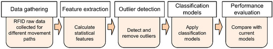
Figure 1. Radio frequency identification (RFID) readings based on classification models.

Several pallet movement scenarios were identified to investigate false positives. Figure 2a shows static and movement RFID tag examples that feasibly occur in actual warehouses. The RFID reader and antenna were installed in the warehouse exit gate before products were loaded in the vehicle. The main system purpose is to accurately record only those tags moved through the gate and subsequently loaded in the vehicle. However, the RFID reader could potentially read moved or static tags, where the moved tags could pass through the gate or close to the gate.

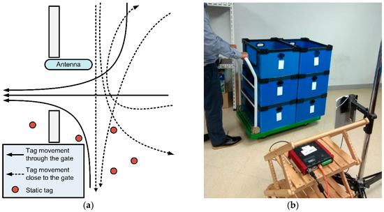
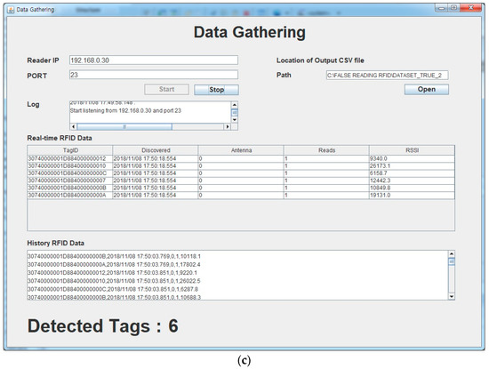
Figure 2. Data gathering: (a) Possible tag movements and static tag locations, (b) example tag movement through the gate, and (c) data gathering program to record tag RSS, etc.

This study considered true positive and false positive RFID readings. True positive readings were defined as the tags read when the pallets were moved through the gate and loaded onto the vehicle; whereas false positives were where pallets were moved close to the gate and the tags were read, but were not loaded onto the vehicle, or pallets were stationary within the reading range of the RFID reader. These accidental reads occur when the tags are located within the nominal read range or the range can be extended accidentally by metal objects within the field [21]. The purpose of the proposed classification model was to identify false positive tags based on extracted RSS information.

Figure 2b shows a typical case where tagged products are moved through the gate. The tags read by the RFID reader through the antenna, and the tag data is forwarded to the client computer through wired connection. We developed the data gathering program to receive and present tag information as well as RSS data in real-time, as shown in Figure 2c. It took approximately 5 s to move the trolley through the gate, and the real-time tags and corresponding RSS details were presented on the screen (Figure 2c) and recorded during this gathering session.

We used 86 × 54 × 1.8 mm card type passive RFID tags for this trial, with the tags attached to the boxes and the trolley moved through the gate at different paths and speeds. The ultra high frequency (UHF) passive RFID tag model was 9662 with frequency 860–960 MHz. The IC type was Alien H3 while protocol was EPC Class1 Gen2 (ISO 18000-6C). The tag was packed with PVC material into a card-type passive tag. In addition, single reader ALR-9900+ from Alien Technology and linear antenna ALR-9610-AL with 5.90 dbi Gain were utilized in this experiment. The operating frequency of the reader was 902–928 MHz and supported EPC Class1 Gen2 (18000-6C). The ALR-9900+ is an enterprise reader, allowing users to monitor or read multiple tags as well as gather RSS data simultaneously at large distances. The Alien reader provides inventory command, a full-featured system for discerning the IDs of multiple tags in the field at the same time. In order to achieve good inventory performance, the reader can dynamically adjust the Q parameter to cause more or fewer tags to respond at any given time. The reader provides several modulation modes available with the Gen2 protocol, such as FM0, M4 (Miller 4), and the default RF mode value is 25M4 [46,47]. To simplify the experiment process, we used default parameters provided by the reader. The reader provided a standard development kit incorporating several languages (Java, Net, Ruby), which allowed relatively simple integration into the developed data gathering program.

During the gathering session, different tags movement paths and speeds through the gate were implemented and performed, and the reading data labelled as true positive. Various other tag movements close to the gate were also conducted and labelled as false positive, and random static tags were placed within the configured read range and also labelled as false positive. In total, 1624 unique data readings were collected, with 1130 false positives and the remainder true positive. Each reading consisted of tag id, date and time, and RSS value. The minimum, maximum, and average number of tags read during a data gathering session where 17, 240, and 69.23, respectively.

Figure 3 shows RSS readings for a typical data gathering session. The ALR-9900+ reader does not provide the unit of measure for the RSSI; therefore, we have presented signal quality (%) as secondary y-axis. First, we investigated the minimum as well as maximum values of RSSI during our experiment, they were 432 and 37,131, respectively. Based on this information, the real value of RSSI was then converted into signal quality (%). The maximum RSS for tags moved through the gate was larger than for static tags (Figure 3a). RSS increased when tags passed through the gate, achieving maximum when the tags were closest to the antenna. In contrast, static tags had relatively constant RSS, since the distance between the antenna and static tag was fixed. This particular case shows a static tag located relatively distant from the reader, hence RSS was low. Figure 3b shows RSS histograms for typical static tags and those moved through the gate. Static tags tended to have small variance, whereas tags moved through the gate tag tended to exhibit heavy-tailed distribution.

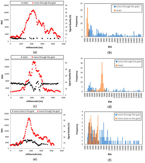
Figure 3. Typical tag RSS and corresponding histogram: (a,b) Relatively distant static and through the gate, (c,d) relatively close static and through the gate, and (e,f) close to the gate and through the gate.

Figure 3c shows the case for a static tag located a relatively close distance to the RFID reader. The static tag generated a non-constant RSS, being relatively stable but reducing when other products being moved through the gate blocked the antenna signal (the worker as well as the boxes). Once the worker and boxes complete passing the gate, the static tag RSS became stable again. Consequently, closer static tags tended to generate histograms with higher variance and maximum RSS values compared to more distant tags (Figure 3b), as shown in Figure 3d. However, closer static tags still tended to have lower variance and light-tailed distributions compared with tags moved through the gate.

Figure 3e shows a typical RSS distribution for a tag moved close to the gate, which is quite similar to that for tags moved through the gate. For both tags, RSS increased as they moved closer to the antenna, then decreased as the distance increased. However, maximum RSS for tags moved close to the gate was lower than for tags moved through the gate, since the antenna did not directly face the tags moved close to the gate. Figure 3f compares typical histograms for tags moved close to and through the gate. Although the histograms are similar, tags moved through the gate tag exhibited higher variance and more heavy-tailed distributions compared to tags moved close to the gate.

Since RSS depends on the distance between the antenna and tag, closer tags generated larger RSS. Therefore, RSS attributes provide important data to classify RFID readings, and have been utilized in previous studies to identify RFID readings with high performance accuracy [20,21,22]. Table 1 shows the nine relevant statistical features extracted from RSS to help distinguish between true and false positives.

Table 1. Attributes extracted from RSS.

Feature	Description
Min	Minimum signal strength during a gathering session
Max	Maximum signal strength during a gathering session
Mean	Average signal strength during a gathering session
Var	RSS variance during a gathering session
Std	RSS standard deviation during a gathering session
Skewness	Distribution asymmetry
Kurtosis	Indicates if the data distribution is heavy- or light-tailed, relative to normal
Diff	Difference between highest and lowest signal strength during a gathering session
Count	Total number of reads for the tag during a gathering session.

During data gathering, the worker loaded several boxes with attached tags on the trolley and performed different RFID readings (i.e., true and false positives) (Figure 2b). To generate a complex dataset, the worker followed different speeds and paths. The data gathering program (Figure 2c), received RSS for each tag through the gathering session, and the raw data was stored as a CSV file. For true positive readings, the worker performed multiple gathering sessions, moving the tags through the gate, and RSS values for static tags located within read range were also collected to generate false positives. Different movement paths and speeds were also performed for tags moved close to the gate.

Table 2 showed the detail execution parameters for gathering the true positive readings (tag movements through the gate), such as number of boxes/tags and the speed and movement pattern of trolley. During gathering session, different numbers of boxes were loaded on the trolley and different numbers of movements through the gate were conducted. In addition, different speeds and paths of the trolleys moving through the gate were considered for data gathering. Based on Table 2, most of the experiments were performed with four tagged boxes on the trolley, with the speed between 0.5–0.99 m/s, and moves straight ahead. In our experiment, the distance between start point (when the tag is first read) and end point (last occurrence of tag) was approximately 4 m.

Table 2. Execution parameters for gathering the true positive readings.

Parameter	Value	Frequency
Number of boxes/tags	1	17
	2	15
	3	12
	4	53
	5	11
	6	24
Speed of trolley (m/s)	<0.50	84
	0.50–0.99	216
	1.00–1.50	155
	1.51–2.00	34
	>2.00	5
Movement pattern	Straight ahead	410
	Diagonal line	84

Figure 4 shows that the raw RFID data, recorded for each gathering session, consisted of the electronic product code (i.e., the tag ID), date and time, antenna information, read time, and RSS. Each raw RFID dataset was then divided based on the tag ID, statistical features to represent data characteristics, and class attributes, labelled as either true positive (1) or false positive (0).

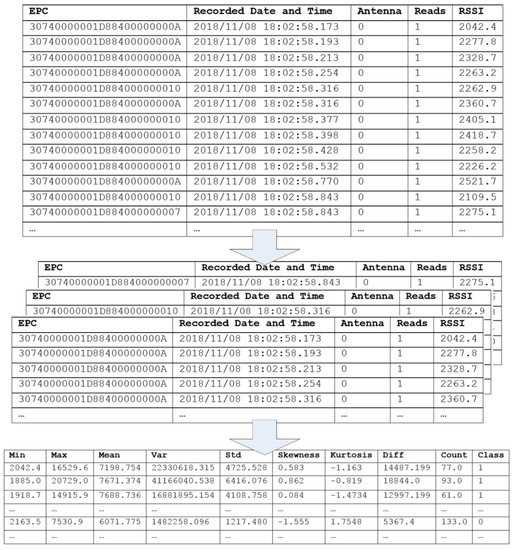
Figure 4. Example of raw RFID data transformation.

Table 3 compares classification accuracy for individual features based on decision stumps (decision trees with single input features). Although each feature can identify true and false positives, none of the features achieved accuracy >90% individually. Thus, a single predictor could not achieve a satisfactory result. However, we expect that combining multiple predictors using machine learning models would significantly improve the prediction performance.

Table 3. Prediction accuracy using individual features.

Predictor	Accuracy
Min	85.591%
Max	89.532%
Mean	69.581%
Var	89.532%
Std	89.532%
Skewness	75.185%
Kurtosis	70.566%
Diff	89.594%
Count	75.431%

4. Classification and Outlier Detection Models

This section describes the process of removing outliers and the machine learning models to classify RFID readings. We used IQR and LOF to identify and, hence, remove outlier data, and then applied several machine learning algorithms: Naïve Bayes (NB), MLP, SVM, DT, and RF.

4.1. Interquartile Range

Outlier detection identifies sample data with different behavior from expected. Most outlier detection methods are based on statistical approaches, acquiring a fitted model from the dataset and identifying outliers as data points in low-probability regions. The IQR approach divides the data set into lower (Q1), median (Q2), and upper (Q3) quartiles, and defines IQR = Q3 − Q1. Data points with values Q1 − (OF × IQR) or Q3 + (OF × IQR) (where OF is the outlier factor) are considered to be outliers [48]. Thus, the total number of outliers depends on the OF parameter. Low OF will generate larger number of outliers, and vice versa. Table 4 shows IQR outlier detection applied to the dataset for two indicative OF values. Assuming normal distributions, the region between the low and high thresholds for OF = 1.5 (i.e., between Q1 − 1.5 × IQR and Q3 + 1.5 × IQR) contained 99.3% of the data points. Therefore, we selected OF = 1.5, retaining 1358 data points (from 1624) for classification.

Table 4. Optimal interquartile range outlier detection.

Original Dataset	Outlier Factor	Outlier Data Points	Acceptable Data Points
1624	1.5	266	1358
	3	135	1489

4.2. Local Outlier Factor

The LOF detection method calculates the local density deviation for a given data point with respect to its neighbors to indicate the degree a data point is an outlier [48,49]. The LOF score for acceptable data is expected to be close to 1, and increases for outliers. The algorithm first calculates the relative density, o, for the dataset, D, and the distance $dis{t}_k\left(o\right)$ between o and another object, p $\in$ D, such that

• There are at least k objects $o^{\prime }$ $\in$ D–{o} such that dist(o, $o^{\prime }$) $\le$ dist(o, $p$), and
• There are at most k − 1 objects $o^{″}\in$ D–{o} such that dist(o, $o^{″}$) < dist(o, $p$).

The k-distance neighborhood of o contains all objects where distance to o < $dis{t}_k\left(o\right),$

$$N_k\left(o\right)=\left\{o^{\prime }|o^{\prime }\in D,dist\left(o,o^{\prime }\right)\le dis{t}_k\left(o\right)\right\}$$

(1)

where $N_k\left(o\right)$ may contain more than k objects. The reachability distance from $o^{\prime }$ to o is

$$reachdis{t}_k\left(o\leftarrow o^{\prime }\right)=max\left\{dis{t}_k\left(o\right),dist\left(o,o^{\prime }\right)\right\}$$

(2)

and the local reachability density, lrd, of an object, o, is

$$lr{d}_k\left(o\right)=\frac{\Vert N_k\left(o\right)\Vert }{{{\displaystyle \sum }}_{o^{\prime }\in N_k\left(o\right)}reachdis{t}_k\left(o^{\prime }\leftarrow o\right)}$$

(3)

Thus, LOF for o is the average of the lrd ratio for the object and k-nearest neighbors,

$$LO{F}_k\left(o\right)=\frac{{{\displaystyle \sum }}_{o^{\prime }\in N_k\left(o\right)}\frac{lr{d}_k\left(o^{\prime }\right)}{lr{d}_k\left(o\right)}}{\Vert N_k\left(o\right)\Vert }$$

(4)

Thus, we could calculate $LO{F}_k$ for all objects in the dataset. The approach takes the single parameter MinPts, the number of nearest neighbors defining the local neighborhood for an object. Previous study provided the guideline on picking the value of MinPts between MinPtsLB (lower bound) and MinPtsUB (upper bound) range [49]. In their experiment, mostly they utilized range value of MinPts between 10 and 50, which appeared to work well in general. We ran the experiment by using MinPtsLB and MinPtsUB as 10 and 40, respectively. The LOF score minimum, maximum, average, and standard deviation = 0.975, 5.064, 1.27, and 0.401, respectively.

A suitable LOF score threshold is required to classify a given data point as outlier or not. Breunig et al. (2000) showed that LOF ≈ 1 should not be considered an outlier [48], and since the LOF distribution was approximately normal (see Figure 5a), 99.7% of the data points fell within $\mu \pm 3\sigma$ (where σ and μ are standard deviation and mean, respectively). Therefore, we set the LOF threshold = $\mu +3\sigma$ = 2.473, as shown in Figure 5a. Table 5 shows the number of outliers identified, and Figure 5b shows where these outlier data occurred in terms of the RSS features defined above.

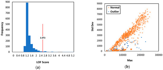
Figure 5. Collected dataset: (a) Local outlier factor (LOF) score, and (b) identified outliers in terms of defined RSS parameters.

Table 5. Optimal local outlier factor (LOF) outlier detection.

Original Dataset	LOF Threshold	Outlier Data Points	Acceptable Data Points
1624	2.473	38	1586

4.3. Naïve Bayes

Naïve Bayes is a statistical classifier that calculates the probability of a given data point belonging to a particular class [48]. Let D be a training dataset and their class. Suppose there are m classes, $C_1$, $C_2$, …, $C_m$. Given a tuple, X, the classifier will predict that X belongs to class $C_i$ with the highest posterior probability, conditioned on X, i.e.,

$$P(C_i|X)>P(C_j|X)\mathrm{for}1\le j\le m,j\ne i$$

(5)

Therefore, we maximize $P(C_i|X)$,

$$P\left(C_i|X\right)=\frac{P\left(X|C_i\right)P\left(C_i\right)}{P\left(X\right)}$$

(6)

The NB classifier performance is comparable with decision tree and can provide high accuracy and speed when applied to large datasets.

4.4. Multilayer Perceptron

The MLP model comprises an ANN with one input layer, one or more hidden layers, and one output layer. The backpropagation algorithm is utilized to train the MLP [48,50]. Figure 6 shows an example MLP, where each layer is composed of several units, corresponding to measured attributes for each training tuple.

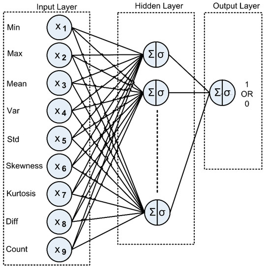
Figure 6. Multilayer perceptron model for RFID classification.

The Min, Max, Mean, Var, Std, Skewness, Kurtosis, Diff, and Count extracted from the RFID reading dataset (see Table 1) were presented as training data to the input layer, passed across the hidden layer, and then to the output layer. Net input was calculated by multiplying each input and its corresponding weight, and then summed. Each unit in the hidden layer took net input and then applied an activation function. Backpropagation compared the prediction result with the target class value, and modified the weights for each training tuple to minimize mean squared error between prediction and target values. This process was iterated multiple times to produce optimal weights, providing optimal predictions for the test data.

4.5. Support Vector Machine

The SVM classifies training data by nonlinearly mapping the original data into high dimensional feature space and finding the linear optimal hyperplane to separate instances each class from the others [48,51]. For the case of separating training vectors belonging to two linearly separable classes,

$$\left(x_i,y_i\right),x_i\in R^n,y_i\in \left\{+1,-1\right\}, i=1,\dots ,n,$$

(7)

where $x_i$ is a real valued n-dimensional input vector and $y_i$ is the class label associated with the training vector. The separating hyperplane is determined by an orthogonal vector $w$ and bias b that identify points that satisfy

$$w·x+b=0$$

(8)

Thus, the classification mechanism for SVM can be expressed as [52,53]

$$ma{x}_{\mathsf{\alpha }}\left[{\displaystyle \sum }_{i=1}^n{\mathsf{\alpha }}_i-\frac{1}{2}{\displaystyle \sum }_{i,j=1}^n{\mathsf{\alpha }}_i{\mathsf{\alpha }}_j{y}_i{y}_{j}K\left(x_i,x_j\right)\right]$$

(9)

with constraints

$${\displaystyle \sum }_{i=1}^n{\mathsf{\alpha }}_i{y}_j=0,\hspace{1em}0\le {\mathsf{\alpha }}_i\le C, i=1,2,\dots .,n$$

(10)

where $\mathsf{\alpha }$ is the parameter vector for the classifier hyperplane, K is a kernel function to measure the distance between $x_i$ and $x_j$, and C is a penalty parameter to control the number of misclassifications. This study used the polynomial kernel function,

$$k\left(x_i,x_j\right)={\left(x_i·x_j+1\right)}^q,q=1,2,\dots ,n.$$

(11)

4.6. Decision Tree

The DT classifier is a tree-like model that illustrates all possible decision alternatives and corresponding outcomes. We used the C4.5 algorithm developed by Ross Quinlan to generate the decision tree [48]. For each tree node, C4.5 selected the attribute that best discriminated the tuples according to class. Let D be the training dataset, then the C4.5 algorithm is shown in Algorithm 1.

Algorithm 1			: C4.5(D)
Input			: dataset D
Output			: Tree
Create node N
Find the best attribute $a_{best}$ that best differentiates instances in D
Label node N with $a_{best}$
for each outcome j of N
	let $D_j$ be the set of data tuples in D that satisfy outcome j
	if$D_j$ is empty then
		attach a leaf labeled with the majority class in D to node N
	else attach the node returned by C4.5 ($D_j$) to node N
end for
returnN

4.7. Random Forest

The RF classifier consists of a collection or ensemble of simple tree predictors, and uses the bagging or random space method [54]. Randomization is introduced by bootstrap sampling the original data and at the node level when growing the tree. RF chooses a random subset of factors at every node and uses them as contenders to locate the best split for each node. Algorithm 2 shows RF generation for each tree.

Algorithm 2		: Random forest
Input		: dataset D, ensemble size T, subspace dimension d
Output		: average prediction from tree models
fort = 1 to T do
	Build a bootstrap sample $D_t$ from D
	Select d features randomly and reduce dimensionality of $D_t$ accordingly
	Train a tree model $M_t$ on $D_t$
	Split on the best feature in d
	Let $M_t$ grow without pruning
end

4.8. Performance Metric

The various classification models to predict RFID reading type are detailed above, and in each case the output class is labelled as 1 (true positive) (i.e., tag moved through the gate), or 0 (false positive) (i.e., tag was static or moved close to the gate). Table 6 shows the confusion matrix, a useful tool to analyze classifier performance. True positive (TP) and true negative (TN) represent tags that are correctly classified, whereas false positive (FP) and false negative (FN) represent tags incorrectly classified.

Table 6. Classifier confusion matrix.

Actual Class	Predicted as “1”	Predicted as “0”
1	TP	FN
0	FP	TN

We employed 10-fold cross-validation for all classification models when generating the models, and the IQR and LOF outlier detection as well as the classification models were implemented in Weka V3.8.0 [55]. Table 7 shows the classification model performance metrics, based on the average value for all cross-validations.

Table 7. Classifier model performance metrics.

Metric	Formula
Precision	$\frac{\mathrm{TP}}{\left(\mathrm{TP}+\mathrm{FP}\right)}$
Recall	$\frac{\mathrm{TP}}{\left(\mathrm{TP}+\mathrm{FN}\right)}$
F-1 score	$\frac{2\times \left(\mathrm{Precision}\times \mathrm{Recall}\right)}{\left(\mathrm{Precision}+\mathrm{Recall}\right)}$
Accuracy	$\frac{\left(\mathrm{TP}+\mathrm{TN}\right)}{\left(\mathrm{TP}+\mathrm{TN}+\mathrm{FP}+\mathrm{FN}\right)}$

5. Results and Discussion

The machine learning models classify RFID readings and can be utilized to improve warehouse management. This section evaluates the classification models and describes how to integrate them into a real-time monitoring system.

5.1. Classification Model Performance

Table 8 compares various model performances, including outlier detection impacts. The machine learning models, such as support vector machine (SVM), multilayer perceptron (MLP), Naïve Bayes (NB), decision tree (DT), and random forest (RF) are utilized to detect false positive readings. The result showed that for conventional models, RF outperformed all other models in terms of precision, recall, F1 score, and accuracy (97.078%, 96.199% 96.623%, and 97.167%, respectively).

Table 8. Classification model performances.

Classifier Model	Recall	F-1 Score	Precision	Accuracy
NB	89.578	89.308	89.054	90.887
MLP	94.934	95.373	95.845	96.121
SVM	90.69	90.69	90.69	92.118
DT	95.035	94.856	94.683	95.628
RF	96.199	96.623	97.078	97.167
NB + IQR	88.559	86.456	84.774	91.016
MLP + IQR	93.476	93.852	94.24	96.171
SVM + IQR	88.056	87.518	87.01	92.047
DT + IQR	93.179	94.448	95.864	96.613
RF + IQR	95.443	95.968	96.517	97.496
NB + LOF	90.661	90.106	89.606	91.677
MLP + LOF	94.923	95.463	96.051	96.28
SVM + LOF	91.501	91.242	90.995	92.686
DT + LOF	96.158	95.642	95.167	96.343
RF + LOF	96.648	96.942	97.249	97.478

Previous studies comparing machine learning algorithms to predict RFID using RSS showed that high classification accuracy could be achieved [21,22], with SVM providing superior accuracy up to 95.5% [22]. However, the present study considered static tags as well as tags moving close to the gate tag as false positive readings, whereas previous studies only considered static tags. Therefore, this study is expected to better represent the complex real situation.

We also investigated the effect of combining outlier detection (IQR or LOF) and the classification model on accuracy, as shown in Table 8 and Figure 7. The classification model accuracy increased when applying interquartile range (IQR) except for SVM, with the overall average increase = 0.28%; whereas applying local outlier factor (LOF) increased the accuracy for all models, with the overall average increase = 0.51%. Our result showed that by integrating either IQR or LOF with RF provided the same and highest accuracy for our dataset = 97.5%. Integrating outlier detection (IQR or LOF) with the classification model improved classification accuracy in our dataset. Previous studies also showed that by integrating IQR or LOF with the prediction model, it improved the accuracy [29,33]. However, this presented model (RF with IQR or LOF) needs to be performed on different types of datasets, as it might not produce the highest accuracy compared to other models.

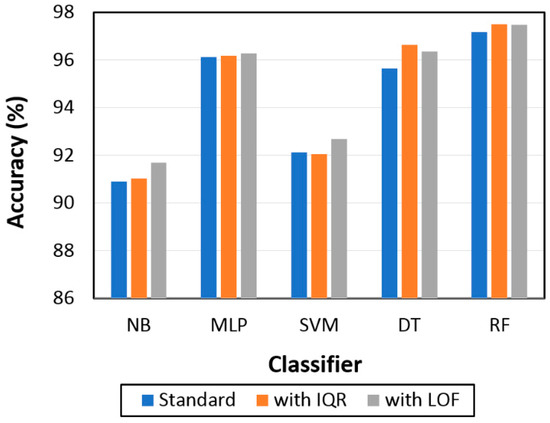
Figure 7. Outlier detection impact on classification model accuracy.

The experimental results indicate that false positive RFID readings can be detected by machine learning with high accuracy. If tags that are static or moved close to the gate are incorrectly classified, the warehouse assumes the relevant products have been loaded. Therefore, incomplete products will be sent. In contrast, when tags moved through the gate are incorrectly classified as static or moved close to the gate, the warehouse will send excess product. Thus, combining outlier detection with suitable classification models will significantly improve the accuracy of WMS monitoring of delivered products to supply chain partners.

5.2. Management Implications

This section describes possible real implementation of false positive detection based on machine learning. Figure 8a shows prototype real-time monitoring system architecture to filter false positives, ensuring only products actually moved through the gate are sent to the representational state transfer application programming interface (REST API), for presentation in web dashboard(s) and/or database storage. We used the MongoDB V3.4.9 database since it can efficiently store continuously-generated sensor/RFID data from manufacturing [56,57,58], healthcare [59], and supply chain [60]. The real-time monitoring system used java programming language V1.8.0 to receive tag information from the readers, filter false positives using trained RF, and send products moved through the gate information to the server via REST API. We used RF since it exhibited significantly superior prediction performance, as detailed in Section 5.

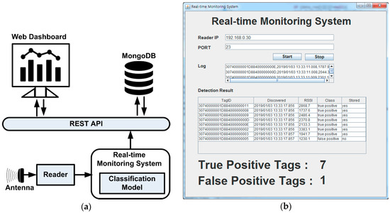
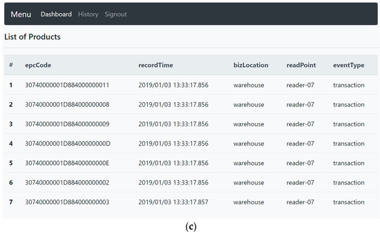
Figure 8. Prototype of real-time monitoring system: (a) System architecture, (b) client program to filter false positives, and (c) web dashboard presents the delivered products.

The REST API used Node.js V8.4.0, Express.js V4.13.4, Bootstrap V4.1.3, and Socket.io V2.1.1. Node.js as the webservers, with Express.js and Bootstrap or data visualization. Socket.io was also used to handle and present product information in real-time. Figure 8b shows the prototype real-time monitoring system receiving tags information from reader and filtering false positives. We assumed the time required to move through the gate before loading was 5 s. Therefore, RSS was gathered for 5 s from when the tag was first read. The collected RSS data was then converted into statistical features (see Section 3) and the trained RF model (see Section 5) applied to detect the tag as true or false positive. False positive tags were filtered and not stored in the server-side database.

Once the tag data was sent to the REST API, product information was presented to the web dashboard and stored into the MongoDB, as shown in Figure 8c. Menu history was available to the user to check historical product data, and the web dashboard enabled managers to monitor product delivered to supply chain partners.

6. Conclusions and Future Work

Detecting and filtering false positives will improve WMS monitoring accuracy for product delivery to supply chain partners. This study used machine learning to predict false positives based on tag RSS. Different tag movement paths and speeds were considered, and statistical features were extracted from tag RSSs. Outlier detection methods were implemented to filter outliers from the collected dataset, and machine learning models were applied to detect static tags and movement close to the gate as false positives. Experimental results showed that integrating outlier detection with machine learning improved classification accuracy. The most accurate classification (97.5%) was achieved by combining LOF or IQR with RF, and was significantly superior to the other combinations and models considered.

We demonstrated the proposed classification model integrated into a prototype real-time monitoring system, comprising a client program to receive tag information from the reader and a REST API to store the information in the cloud. The client program also filtered false positives to ensure only correct product details (i.e., true positive tag readings), and were forwarded to the REST API and stored in the database. Thus, managers could monitor products delivered to supply chain partners in real-time using the prototype web-based monitoring system.

Future study should consider different parameters as addition to RSSI, such as phase and doppler, as well as utilizing multiple readers or antennas. The datasets that better represent complex real situations, such as by considering different tag orientations and tag movement directions, need to be gathered in the near future. Furthermore, extending the comparison with other classification models, as well as applying machine learning models to identify other problems that occur during RFID readings, such as false negative readings or miss-reads, could be presented in the near future.

References

- Yang, S.; MR, A.; Kaminski, J.; Pepin, H. Opportunities for Industry 4.0 to Support Remanufacturing. Appl. Sci. 2018, 8, 1177. [Google Scholar] [CrossRef]
- Álvarez López, Y.; Franssen, J.; Álvarez Narciandi, G.; Pagnozzi, J.; González-Pinto Arrillaga, I.; Las-Heras Andrés, F. RFID Technology for Management and Tracking: E-Health Applications. Sensors 2018, 18, 2663. [Google Scholar] [CrossRef]
- Pérez, M.M.; González, G.V.; Dafonte, C. The Development of an RFID Solution to Facilitate the Traceability of Patient and Pharmaceutical Data. Sensors 2017, 17, 2247. [Google Scholar] [CrossRef] [PubMed]
- Martínez Pérez, M.; Dafonte, C.; Gómez, Á. Traceability in Patient Healthcare through the Integration of RFID Technology in an ICU in a Hospital. Sensors 2018, 18, 1627. [Google Scholar] [CrossRef] [PubMed]
- Zhu, L.; Lee, C. Risk Analysis of a Two-Level Supply Chain Subject to Misplaced Inventory. Appl. Sci. 2017, 7, 676. [Google Scholar] [CrossRef]
- Parsons, A.; Cooper, J.; Onda, Y.; Sakai, N. Application of RFID to Soil-Erosion Research. Appl. Sci. 2018, 8, 2511. [Google Scholar] [CrossRef]
- Kang, Y.-S.; Kim, H.; Lee, Y.-H. Implementation of an RFID-Based Sequencing-Error-Proofing System for Automotive Manufacturing Logistics. Appl. Sci. 2018, 8, 109. [Google Scholar] [CrossRef]
- de Souza, P.; Marendy, P.; Barbosa, K.; Budi, S.; Hirsch, P.; Nikolic, N.; Gunthorpe, T.; Pessin, G.; Davie, A. Low-Cost Electronic Tagging System for Bee Monitoring. Sensors 2018, 18, 2124. [Google Scholar] [CrossRef]
- Fernández-Caramés, T.M.; Fraga-Lamas, P.; Suárez-Albela, M.; Díaz-Bouza, M.A. A Fog Computing Based Cyber-Physical System for the Automation of Pipe-Related Tasks in the Industry 4.0 Shipyard. Sensors 2018, 18, 1961. [Google Scholar] [CrossRef]
- Syaekhoni, M.A.; Alfian, G.; Kwon, Y.S. Customer Purchasing Behavior Analysis as Alternatives for Supporting In-Store Green Marketing Decision-Making. Sustainability 2017, 9, 2008. [Google Scholar] [CrossRef]
- Bunker, R.; Elsherbeni, A. A Modular Integrated RFID System for Inventory Control Applications. Electronics 2017, 6, 9. [Google Scholar] [CrossRef]
- Shih, C.-H.; Juang, J.-G. Moving Object Tracking and Its Application to an Indoor Dual-Robot Patrol. Appl. Sci. 2016, 6, 349. [Google Scholar] [CrossRef]
- Ma, L.; Liu, M.; Wang, H.; Yang, Y.; Wang, N.; Zhang, Y. WallSense: Device-Free Indoor Localization Using Wall-Mounted UHF RFID Tags. Sensors 2019, 19, 68. [Google Scholar] [CrossRef] [PubMed]
- Liu, F.; Zhong, D. GSOS-ELM: An RFID-Based Indoor Localization System Using GSO Method and Semi-Supervised Online Sequential ELM. Sensors 2018, 18, 1995. [Google Scholar] [CrossRef] [PubMed]
- Wang, C.; Shi, Z.; Wu, F. Intelligent RFID Indoor Localization System Using a Gaussian Filtering Based Extreme Learning Machine. Symmetry 2017, 9, 30. [Google Scholar] [CrossRef]
- Seco, F.; Jiménez, A.R. Smartphone-Based Cooperative Indoor Localization with RFID Technology. Sensors 2018, 18, 266. [Google Scholar] [CrossRef]
- Shen, B.; Zheng, Q.; Li, X.; Xu, L. A Framework for Mining Actionable Navigation Patterns from In-Store RFID Datasets via Indoor Mapping. Sensors 2015, 15, 5344–5375. [Google Scholar] [CrossRef]
- Hsu, C.-C.; Chen, J.-H. A Novel Sensor-Assisted RFID-Based Indoor Tracking System for the Elderly Living Alone. Sensors 2011, 11, 10094–10113. [Google Scholar] [CrossRef]
- Jayatilaka, A.; Ranasinghe, D.C. Real-time fluid intake gesture recognition based on batteryless UHF RFID technology. Pervasive Mob. Comput. 2017, 34, 146–156. [Google Scholar] [CrossRef]
- Keller, T.; Thiesse, F.; Kungl, J.; Fleisch, E. Using low-level reader data to detect false-positive RFID tag reads. In Proceedings of the 2010 Internet of Things (IOT), Tokyo, Japan, 29 November–1 December 2010; pp. 1–8. [Google Scholar]
- Keller, T.; Thiesse, F.; Fleisch, E. Classification models for RFID-based real-time detection of process events in the supply chain: An empirical study. Acm Trans. Manag. Inf. Syst. (TMIS) 2015, 5, 25. [Google Scholar] [CrossRef]
- Ma, H.; Wang, Y.; Wang, K. Automatic detection of false positive RFID readings using machine learning algorithms. Expert Syst. Appl. 2018, 91, 442–451. [Google Scholar] [CrossRef]
- Hauser, M.; Zügner, D.; Flath, C.M.; Thiesse, F. Pushing the limits of RFID: Empowering RFID-based Electronic Article Surveillance with Data Analytics Techniques. In Proceedings of the 2015 Thirty Sixth International Conference on Information Systems, Fort Worth, TX, USA, 13–16 December 2015. [Google Scholar]
- Hauser, M.; Günther, S.A.; Flath, C.M.; Thiesse, F. Towards Digital Transformation in Fashion Retailing: A Design-Oriented IS Research Study of Automated Checkout Systems. Bus. Inf. Syst. Eng. 2018. [Google Scholar] [CrossRef]
- Yao, H.; Fu, X.; Yang, Y.; Postolache, O. An Incremental Local Outlier Detection Method in the Data Stream. Appl. Sci. 2018, 8, 1248. [Google Scholar] [CrossRef]
- Yang, Y.; Liu, Q.; Gao, Z.; Qiu, X.; Meng, L. Data Fault Detection in Medical Sensor Networks. Sensors 2015, 15, 6066–6090. [Google Scholar] [CrossRef] [PubMed]
- Lee, J.; Kang, B.; Kang, S.H. Integrating independent component analysis and local outlier factor for plant-wide process monitoring. J. Process Control 2011, 21, 1011–1021. [Google Scholar] [CrossRef]
- Song, B.; Shi, H.; Ma, Y.; Wang, J. Multisubspace principal component analysis with local outlier factor for multimode process monitoring. Ind. Eng. Chem. Res. 2014, 53, 16453–16464. [Google Scholar] [CrossRef]
- Zhao, S.; Li, W.; Cao, J. A User-Adaptive Algorithm for Activity Recognition Based on K-Means Clustering, Local Outlier Factor, and Multivariate Gaussian Distribution. Sensors 2018, 18, 1850. [Google Scholar] [CrossRef] [PubMed]
- Do, H.; Cetin, K.S. Evaluation of the causes and impact of outliers on residential building energy use prediction using inverse modeling. Build. Environ. 2018, 138, 194–206. [Google Scholar] [CrossRef]
- Jeong, J.; Park, E.; Han, W.S.; Kim, K.; Choung, S.; Chung, I.M. Identifying outliers of non-Gaussian groundwater state data based on ensemble estimation for long-term trends. J. Hydrol. 2017, 548, 135–144. [Google Scholar] [CrossRef]
- van Capelleveen, G.; Poel, M.; Mueller, R.M.; Thornton, D.; van Hillegersberg, J. Outlier detection in healthcare fraud: A case study in the Medicaid dental domain. Int. J. Account. Inf. Syst. 2016, 21, 18–31. [Google Scholar] [CrossRef]
- Sun, S.; Li, G.; Chen, H.; Guo, Y.; Wang, J.; Huang, Q.; Hu, W. Optimization of support vector regression model based on outlier detection methods for predicting electricity consumption of a public building WSHP system. Energy Build. 2017, 151, 35–44. [Google Scholar] [CrossRef]
- Bai, Y.; Wang, F.; Liu, P. Efficiently Filtering RFID Data Streams. In Proceedings of the 1st International Very Large Data Base Workshop on Clean Databases (CleanDB), Seoul, Korea, 11 September 2006; pp. 50–57. [Google Scholar]
- Jeffery, S.R.; Garofalakis, M.; Franklin, M.J. Adaptive cleaning for RFID data streams. In Proceedings of the 32nd international conference on very large data bases (VLDB), Seoul, Korea, 12–15 September 2006; pp. 163–174. [Google Scholar]
- Massawe, L.V.; Kinyua, J.D.M.; Vermaak, H. Reducing False Negative Reads in RFID Data Streams Using an Adaptive Sliding-Window Approach. Sensors 2012, 12, 4187–4212. [Google Scholar] [CrossRef] [PubMed]
- Fazzinga, B.; Flesca, S.; Furfaro, F.; Parisi, F. Offline cleaning of RFID trajectory data. In Proceedings of the 26th International Conference on Scientific and Statistical Database Management—SSDBM’14, Aalborg, Denmark, 30 June–2 July 2014; pp. 1–12. [Google Scholar]
- Fazzinga, B.; Flesca, S.; Furfaro, F.; Parisi, F. Exploiting Integrity Constraints for Cleaning Trajectories of RFID-Monitored Objects. ACM Trans. Database Syst. 2016, 41, 1–52. [Google Scholar] [CrossRef]
- Baba, A.I.; Jaeger, M.; Lu, H.; Pedersen, T.B.; Ku, W.-S.; Xie, X. Learning-Based Cleansing for Indoor RFID Data. In Proceedings of the 2016 International Conference on Management of Data—SIGMOD’16, San Francisco, CA, USA, 26 June–1 July 2016; pp. 925–936. [Google Scholar]
- Tu, Y.J.; Piramuthu, S. A decision-support model for filtering RFID read data in supply chains. IEEE Trans. Syst. Man Cybern. Part C (Appl. Rev.) 2011, 41, 268–273. [Google Scholar] [CrossRef]
- Keller, T.; Thiesse, F.; Ilic, A.; Fleisch, E. Decreasing false-positive RFID tag reads by improved portal antenna setups. In Proceedings of the 2012 3rd IEEE International Conference on the Internet of Things, Wuxi, China, 24–26 October 2012; pp. 99–106. [Google Scholar]
- Buffi, A.; Nepa, P. A phase-based technique for discriminating tagged items moving through a UHF-RFID gate. In Proceedings of the 2014 IEEE RFID Technology and Applications Conference (RFID-TA), Tampere, Finland, 8–9 September 2014; pp. 155–158. [Google Scholar]
- Buffi, A.; Nepa, P. The SARFID Technique for Discriminating Tagged Items Moving Through a UHF-RFID Gate. IEEE Sens. J. 2017, 17, 2863–2870. [Google Scholar] [CrossRef]
- Xu, J.; Yang, L.; Liu, Q.; Hu, J.; Song, T. A sorting algorithm for RFID tags moving on a conveyor belt. In Proceedings of the 2018 IEEE International Conference on RFID (RFID), Orlando, FL, USA, 10–12 April 2018; pp. 1–7. [Google Scholar]
- Tesch, D.A.; Berz, E.L.; Hessel, F.P. RFID indoor localization based on Doppler effect. In Proceedings of the Sixteenth International Symposium on Quality Electronic Design, Santa Clara, CA, USA, 2–4 March 2015; pp. 556–560. [Google Scholar]
- ALR-9900+ Enterprise RFID Reader. Available online: http://www.alientechnology.com/wp-content/uploads/Alien-Technology-ALR-9900-Enterprise-RFID-Reader.pdf (accessed on 3 March 2019).
- Reader Interface Guide ALR-F800, ALR-9900+, ALR-9680, ALR-9650. Available online: ftp://ftp.alientechnology.com/pub/readers/docs/8101938-000_V_Guide,%20Reader%20Interface.pdf (accessed on 3 March 2019).
- Han, J.; Kamber, M.; Pei, J. Data Mining: Concepts and Techniques, 3rd ed.; Morgan Kaufmann Publishers: Burlington, MA, USA, 2011. [Google Scholar]
- Breunig, M.M.; Kriegel, H.P.; Ng, R.T.; Sander, J. LOF: Identifying density-based local outliers. In Proceedings of the 2000 ACM SIGMOD international conference on Management of data, Dallas, TX, USA, 15–18 May 2000; pp. 93–104. [Google Scholar]
- Rumelhart, D.E.; Hinton, G.E.; Williams, R.J. Learning representations by back-propagating errors. Nature 1986, 323, 533–536. [Google Scholar] [CrossRef]
- Cortes, C.; Vapnik, V. Support-vector networks. Mach. Learn. 1995, 20, 273–297. [Google Scholar] [CrossRef]
- Akay, M.F. Support vector machines combined with feature selection for breast cancer diagnosis. Expert Syst. Appl. 2009, 36, 3240–3247. [Google Scholar] [CrossRef]
- Zheng, B.; Yoon, S.W.; Lam, S.S. Breast cancer diagnosis based on feature extraction using a hybrid of K-means and support vector machine algorithms. Expert Syst. Appl. 2014, 41, 1476–1482. [Google Scholar] [CrossRef]
- Breiman, L. Random Forests. Mach. Learn. 2001, 45, 5–32. [Google Scholar] [CrossRef]
- Weka 3: Data Mining Software in Java. Available online: https://www.cs.waikato.ac.nz/ml/weka/ (accessed on 1 November 2018).
- Syafrudin, M.; Fitriyani, N.L.; Li, D.; Alfian, G.; Rhee, J.; Kang, Y.-S. An Open Source-Based Real-Time Data Processing Architecture Framework for Manufacturing Sustainability. Sustainability 2017, 9, 2139. [Google Scholar] [CrossRef]
- Syafrudin, M.; Alfian, G.; Fitriyani, N.L.; Rhee, J. Performance Analysis of IoT-Based Sensor, Big Data Processing, and Machine Learning Model for Real-Time Monitoring System in Automotive Manufacturing. Sensors 2018, 18, 2946. [Google Scholar] [CrossRef] [PubMed]
- Syafrudin, M.; Fitriyani, N.L.; Alfian, G.; Rhee, J. An Affordable Fast Early Warning System for Edge Computing in Assembly Line. Appl. Sci. 2019, 9, 84. [Google Scholar] [CrossRef]
- Alfian, G.; Syafrudin, M.; Ijaz, M.F.; Syaekhoni, M.A.; Fitriyani, N.L.; Rhee, J. A Personalized Healthcare Monitoring System for Diabetic Patients by Utilizing BLE-Based Sensors and Real-Time Data Processing. Sensors 2018, 18, 2183. [Google Scholar] [CrossRef]
- Alfian, G.; Syafrudin, M.; Rhee, J. Real-Time Monitoring System Using Smartphone-Based Sensors and NoSQL Database for Perishable Supply Chain. Sustainability 2017, 9, 2073. [Google Scholar] [CrossRef]
© 2019 by the authors. Licensee MDPI, Basel, Switzerland. This article is an open access article distributed under the terms and conditions of the Creative Commons Attribution (CC BY) license (http://creativecommons.org/licenses/by/4.0/).