Article

Analyzing the Impact of Variability and Uncertainty on Power System Flexibility

Department of Electrical and Electronic Engineering, Joongbu University, 305 Dongheon-ro, Deogyang-gu, Goyang-si, Gyeonggi-do 10279, Korea
Appl. Sci. 2019, 9(3), 561; https://doi.org/10.3390/app9030561
Submission received: 8 January 2019 / Revised: 29 January 2019 / Accepted: 6 February 2019 / Published: 8 February 2019

Abstract

:

Featured Application

This study presents a method for separating the variability and uncertainty in a power system, and determining which is more influential in terms of flexibility, based on the flexibility index, named the ramping capability shortage probability (RSP). A process of scenario generation and sensitivity analysis is also proposed, and applied to a modified IEEE-RTS-96. The proposed method can evaluate the individual effect of variability and uncertainty and effectively provide the system operator with information that will enable more efficient operation and planning of a power system.

Abstract

This study investigates the impact of variability and uncertainty on the flexibility of a power system. The variability and uncertainty make it harder to maintain the balance between load and generation. However, most existing studies on flexibility evaluation have not distinguished between the effects of variability and uncertainty. The countermeasures to address variability and uncertainty differ; thus, applying strategies individually tailored to variability and uncertainty is helpful for more efficient operation and planning of a power system. The first contribution of this study is in separating the variability and uncertainty, and determining which is more influential in terms of flexibility in specific system situations. A flexibility index, named the ramping capability shortage probability (RSP), is used to quantify the extent to which the variability and uncertainty affect the flexibility. The second contribution is to generate various scenarios for variability and uncertainty based on a modified IEEE-RTS-96, to evaluate the flexibility. The penetration level of renewable energy resources is kept the same in each scenario. The results of a sensitivity analysis show that variability is more effective than uncertainty for high and medium net loads.

1. Introduction

In South Korea, wind and photovoltaic (PV) power systems of approximately 41.6 GW installed capacity are planned for construction by 2030, based on the 3020 penetration plan for renewable energy resources. The term “3020” indicates that the ratio of electricity generation by renewable energy resources to total electricity generation should reach a target of 20% by 2030 [1]. Under this plan, the installed capacity of renewable energy resources in Korea in 2030 would be about five times higher than in 2018, and a large proportion of the newly installed renewable energy resources would be wind and PV power systems.
Setting aside the practicality of the plan, large-scale integration of renewable energy resources into power systems may cause flexibility problems [2,3], where flexibility is defined as the ability to respond to changes in net load, i.e., the load subtracted from the power outputs of renewable energy resources. The National Renewable Energy Laboratory (NREL) and the North American Electric Reliability Corporation (NERC) have investigated the flexibility problem in light of the expectation that the penetration of renewable energy resources is likely to increase significantly [4,5]. System operators and planners have begun to encounter this problem, and maintenance of flexibility requires urgent attention.
The flexibility problem has arisen because the outputs of the renewable energy resources, such as wind and PV power systems, are variable and unpredictable [6,7,8]. High penetration of wind and PV power systems increases the variability and uncertainty of the net load, and exacerbates the flexibility problem in power systems. Variability does not involve uncertainty, i.e., no risk is included in calculations of variability [9,10]. If the generation capacity is sufficient to satisfy the forecast net load, the variability of this load can be covered by the scheduled outputs of generating units. However, uncertainties such as the unexpected failure of a generating unit or load forecast errors are inevitable, and these can lead to unsatisfied variability. Reserve capacity is thus usually required for uncertainty-contained situations, and system operators address this possibility by securing an adequate level of reserve capacity [11,12,13,14]. To sum up, the scheduled output and reserve capacity are used as countermeasures for variability and uncertainty, respectively [15]. Tailored responses to variability and uncertainty may be possible by separating the variability and uncertainty [16].
Existing studies on the flexibility problem can be categorized into two types: those that discuss the application of flexible resources, such as energy storage systems, and demand-side resources (DSRs) to mitigate the variability and uncertainty [3,17,18,19,20]; and those that investigate operational methods such as the unit commitment (UC) and power flow to effectively respond to increased variability and uncertainty [21,22,23,24,25,26,27,28]. In the latter category, the effects of variability and uncertainty are restricted using ramp-up/down constraints (collectively known as ramp constraints) in stochastic and deterministic UC formulations [21,22,23,24,25,26]. However, ramp constraints merely guarantee a feasible solution; adequate or optimal flexibility and the trade-off between the available amount of flexible resources and the operating cost are not taken into account. More importantly, the extent to which the variability and uncertainty affect the flexibility has not been explicitly distinguished in those frameworks; existing research [26] has only attempted to quantify the individual effect of variability and uncertainty on flexibility using a proposed index called AACEE, which estimates the power imbalance caused by the variability and uncertainty. However, generator failure was not considered, although this is a major source of uncertainty.
Therefore, in this study, an index called the ramping capability shortage probability (RSP) is used to quantify the individual effect of variability and uncertainty on flexibility. The RSP is able to consider not only the trade-off between the available amount of flexible resources and the operating cost, but also the major uncertainties including generator failure [29]. Based on the RSP, this study presents a method for separating the variability and uncertainty, and determining which is more influential in terms of flexibility. Various scenarios for variability and uncertainty based on a modified IEEE-RTS-96 are generated. In these scenarios, the net load variation and net load forecast error are used as parameters to represent the variability and uncertainty, respectively. The results of sensitivity analysis show that the variability (uncertainty) is more effective than the uncertainty (variability) for high and medium (low) net loads.
The remainder of this paper is organized as follows. Section 2 introduces the RSP flexibility index, which is capable of quantifying flexibility according to variability and uncertainty. Section 3 explains scenario generation to compare the effect of variability and uncertainty on flexibility. In Section 4, a case study for a modified IEEE-RTS-96 is discussed. Conclusions and future work are discussed in Section 5.

2. Flexibility Index: Ramping Capability Shortage Probability

The extent to which variability and uncertainty affect flexibility can be quantified using the RSP flexibility index, which can assist power system operators in managing the flexibility problem. RSP is described in detail in the following section.

2.1. System Ramping Capability (SRC), Ramping Capability Requirement (RCR)

First, the ramping capability (RC) of a generating unit is defined as the generation power that the unit can increase/decrease in a given period of time. The RC can be thought of as the system’s ability to response to increased variability and uncertainty. The flexibility depends on the amount of RC secured. The total RC of all generating units in the system is denoted as the system RC (SRC), given by
S R C t = i I A i , t Δ t O i , t Δ t min ( P max , i P i , t Δ t ,    r r i Δ t ) .
The SRCt indicates the extent to which the system can supply the RC during the interval Δt. The larger the SRC secured, the greater the flexibility; however, uncertainty in the system may lower RC availability. In Equation (1), Ai,t-Δt is a random variable denoting whether the unit fails from t∆t to t.; its value may vary with the failure rate of the generating unit. Further information on the Ai,t-Δt calculation can be found in [30]. Parameters such as Oi,t-Δt and Pi,t-Δt are determined by the generation schedule.
The RC requirement (RCR) can be represented as
R C R t = N L F E t + F N L t i I A i , t Δ t O i , t Δ t P i , t Δ t ,
where
N L F E t   = L F E t V G F E t
F N L t   = F L t F V G t .
RCRt is the total RC required to respond to unexpected load variations and failures of loaded generating units from t∆t to t. The forecast errors NLFEt, LFEt, and VGFEt are random variables.

2.2. Ramping Capability Shortage Probability

If RCRt is larger than SRCt, then load shedding is enforced; this situation is denoted as RC shortage. The probability that an RC shortage will happen at time t is defined as the RC shortage probability (RSPt), is expressed by
R S P t =      e E t P r o b ( e ) [ c C t Δ t P r o b c [ F N L t + N L F E t > i I A i , t Δ t O i , t Δ t { P i , t Δ t + min ( P m a x , i P i , t Δ t , r r i Δ t ) } ] ]
The RSPt is applied to the worst case, i.e., when calculating the RSPt of the targeted time, uncertainty cases are considered that occur just before the targeted time and thus cannot be resolved by post-recovery actions. This consideration is helpful in reducing the computational burden in large power systems. The variability relates to FNLt, Ot-Δt, and Pt-Δt. Any change in FNLt itself indicates an increase/decrease in variability, and also changes Ot-Δt and Pi, t-Δt. Uncertainty is associated with Ct-Δt, Et, At-Δt, and NLFEt, and Ct-Δt and Et represent the set of possible cases for Ai,t-Δt and NLFEt, respectively.
An example for Ct-Δt is as follows: two online generating units are considered for 2 h. Each unit has two states, i.e., 0 (failure) or 1 (online). Considering the possible cases of two units, C1 is a set of four elements; i.e., {(0,0), (0,1), (1,0), (1,1)}. The probability of each element can be obtained based on a Markov-chain–based capacity state model; for further information, please refer to [30]. An example for Et is as follows: the forecast net loads (i.e., FNLt) are assumed to be 10 MW. If NLFEt follows a triangular distribution as shown in Figure 1, Et becomes {(−0.5 MW), (0 MW), (0.5 MW)} by multiplying 10 MW and 5%, and the elements have a probability of 0.25, 0.5, and 0.25, respectively. Therefore, any changes in the parameters relating to the variability and uncertainty can be reflected in the RSPt calculation.
Complementarity is considered an influential factor with respect to the variability of the system [31]. Its effect is reflected in NLFEt, VGFEt, Oi,t-Δt, and Pi,t-Δt. If the aggregated forecast output of renewable energy resources change with the effects of complementarity, the value of FVGt varies, and accordingly the value of VGFEt, leading to changes in Oi,t-Δt, and Pi,t-Δt.

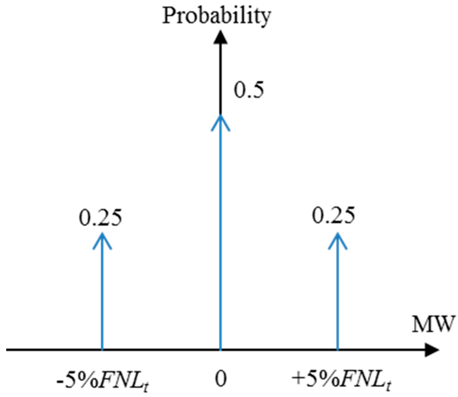
3. Scenarios for Variability and Uncertainty

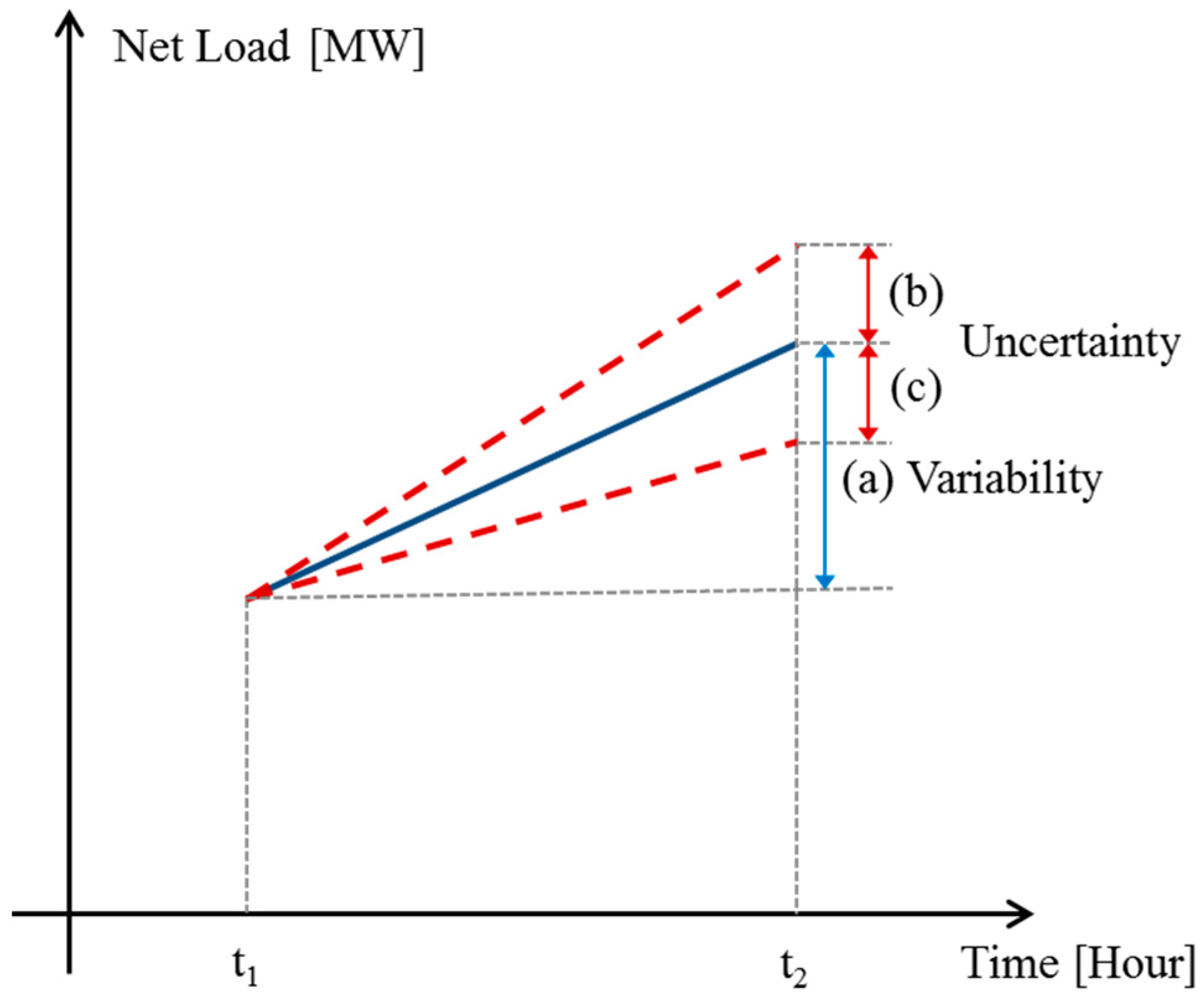
3.1. Variability and Uncertainty and Their Relevance

Variability commonly refers to how dispersed or spread out the data values are. In statistics, there are metrics for describing variability in a dataset: range, interquartile range, variance and standard deviation. The range is a measure of spread: it represents the difference between the highest and lowest values in a dataset. The interquartile range is a measure of where the “middle fifty” is in a dataset, that is, a measure of where the majority of the values lie. The variance is the mean square of the differences from the mean, and the standard deviation is the square root of the variance. These indices enable comparison of data in terms of variability. In power systems, a typical variability is the load variability, which has been represented using the standard deviation.
Uncertainty exists when the measured value differs from the forecast value; uncertainty has been widely represented by the error, which is defined as the measured value minus the forecast value. The net load forecast error and the unexpected failure of generating units are major uncertainties in power systems. Based on a probabilistic approach, these uncertainties have been considered as random variables. The net load forecast error has been modelled as a normal random variable, which follows a normal probability distribution. Without uncertainty, there is no risk related to flexibility; only variability exists. The variation in the forecast net load can be perfectly covered by the scheduled outputs of generating units, and the RC is thus not required. However, in reality, uncertainty always exists and causes risk situations in which RC is required.
It should be noted that uncertainty and variability are linked through the RC. The variation of the forecast net load may alter the operating conditions of generating units; some units may not be involved in the operation. This means that the RC of the system changes with variability; this, of course, changes the system’s ability to respond to risk.

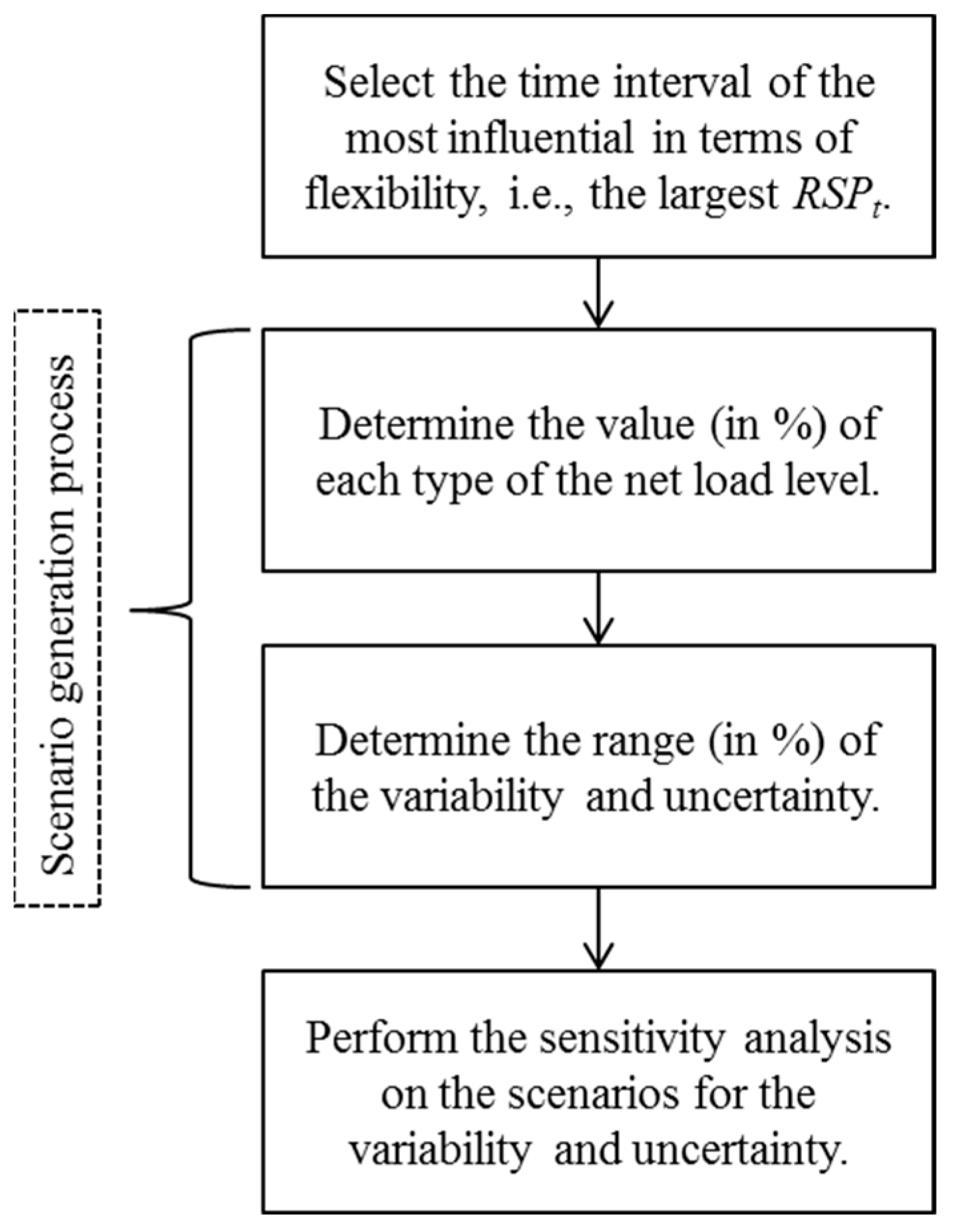
3.2. Scenario Generation and Sensitivity Analysis
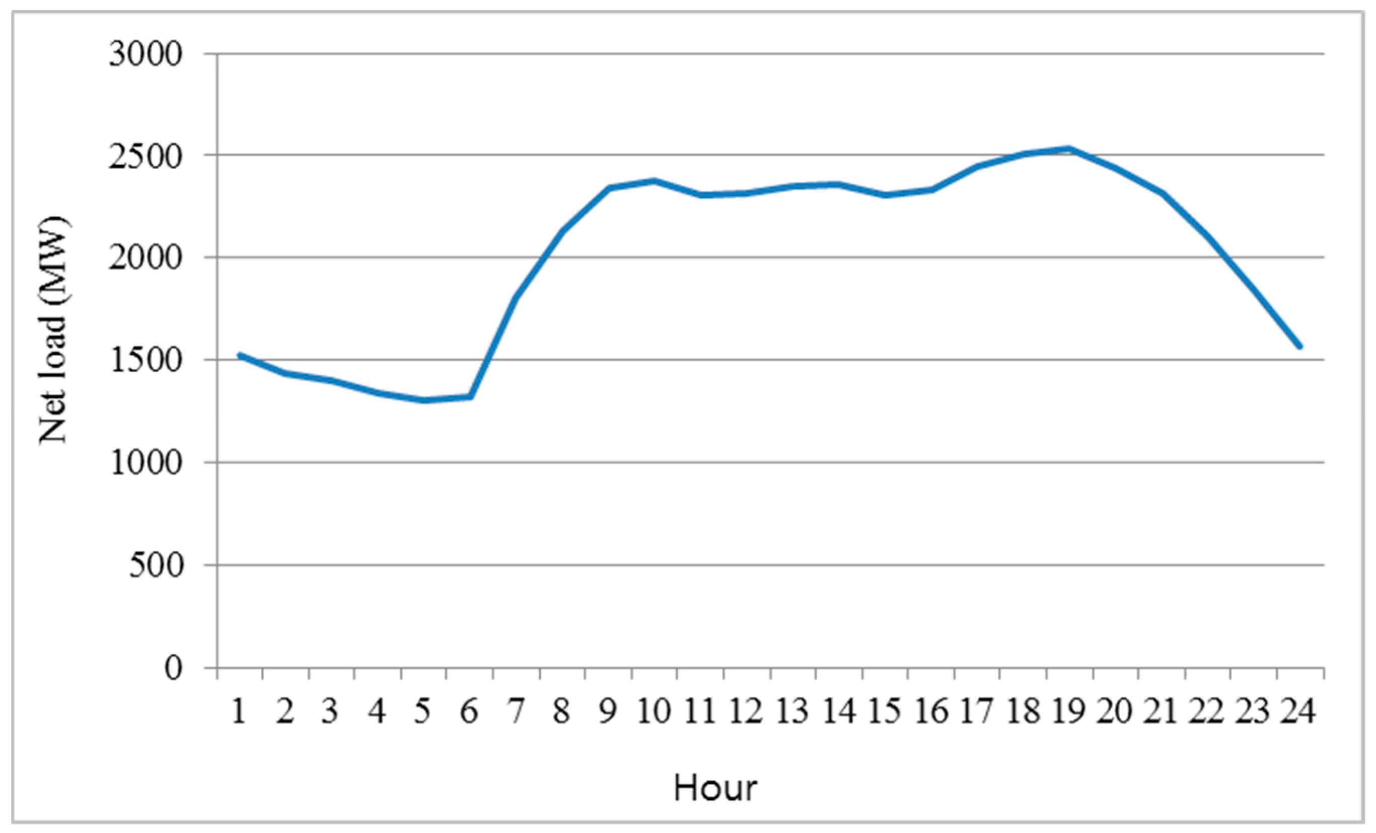
A scenario-based approach is applied in this study. To clarify the impacts of variability and uncertainty, the following are considered. First, the net load variation appears in every time interval. As every time interval is complex, this complicates the analysis of the results. Thus, to enhance the analyzability and clarity, the most influential time interval, in terms of flexibility, is selected and the net load variation for the time interval is varied. RSPt is used as the selection criterion, i.e., the time interval of the largest RSPt is chosen.
Figure 2 represents the forecast net load variation and measured net load variation for the selected time interval. A blue straight line and two red dotted lines for the selected time interval (between t1 and t2) indicate the forecast net load variation and measured net load variation, respectively. (a) means variability, and (b) and (c) imply uncertainty. Differently with the forecast net load variation, the measured net load variation includes uncertainty.
The variability and uncertainty both vary with net load at time t1 and t2. When adjusting the variability, it is assumed that the net load at time t2 is changed, while the net load at time t1 is fixed. This assumption is useful in clarifying scenario generation, and comparing the result of the uncertainty with that of the variability.
The uncertainty is represented by some percentage (indicating the standard deviation expressed as a percentage) of the net load at time t2. A change in the variability is accompanied by a change in the uncertainty, because both parameters are dependent on the net load at time t2. Therefore, to keep the uncertainty unchanged with the variability, the same value of the uncertainty of the base case is applied to all scenarios for the variability; the “base case” refers to the information of the given system.
The scenarios for the increased variability and uncertainty are listed in Table 1. For reference, “increased variability” instead of variability is used for scenario generation; it is represented as an increment based on the variability of the base case, and its value is calculated as some percentage of the net load. The increased variability of the base case is thus equal to zero.
The effects of increased variability and uncertainty on flexibility change with the net load because the reserve capacity of generating units may vary with the net load. The net load is thus classified into three types: high, medium, and low. Among these types, the medium net load corresponds to the base case of the net load (i.e., 100%), and is represented in S3 and S4. The high (low) type is larger (smaller) than 100%, given by S1 and S2 (S5 and S6). Each type depends on the system conditions, e.g., low net load can occur due to use of DSRs in the time period considered. Empirical trials were used to determine the value of each type of net load.
For every net load, two kinds of scenarios for variability and uncertainty are considered: one (the other) is when the variability (uncertainty) is fixed and the uncertainty (variability) is changed. The value of the increased variability is 0% for the fixed case, i.e., S2, S4, and S6. The value of the uncertainty (i.e., the net load forecast error) is set as a particular percentage for the fixed case: i.e., S1, S3, and S5.
For the system conditions, complementarity affects the variability of the system, e.g., if the outputs of two wind power systems with the same capacity are perfectly negatively correlated, i.e., the output of one system increases (decreases) while that of another system decreases (increases) at the same rate, the added variability becomes zero. On the other hand, if they are perfectly positively correlated, the added variability is doubled. The complementarity changes the variability, and thereby the flexibility. Related works were performed in [7]. The correlation between outputs of renewable energy resources may affect the complementarity. In this study, the penetration levels of renewable energy resources in each region are kept the same for every scenario; thus, the complementarity effect was fixed throughout the scenarios.
The increased variability and uncertainty were varied within a given range, which may also differ according to the system conditions. Through the sensitivity analysis, the effects of variability and uncertainty on flexibility can be compared, and the most influential factor determined. The process of scenario generation is summarized in Figure 3.

4. Case Study

4.1. Base Case Information

The main objective is to examine the impacts of variability and uncertainty on flexibility. The test system was a modified IEEE-RTS-96. The generation system consists of 26 generating units, and its installed capacity is 3105 MW. Basic information on the failure and repair rates of generating units is provided in Table A1 (Appendix A). Wind power plants of 1250 MW were added to the system; for reference, their capacity value (based on the effective load carrying capability) was computed as 79.88 MW [32]. Figure 4 shows the profile of the forecast net load, with the 2531 MW peak load occurring at hour 19. The hourly UC was solved using dynamic programming [33]. The hourly reserve capacity was calculated on the assumption that all generating units are in a spinning state; this assumption was used to evaluate the maximum flexibility of the system. The value of RSPt was computed through programming in MATLAB (R2012b version) [34]. This simulation was performed on a PC with 16 GB RAM and 3.7 GHz CPU. As shown in Figure 5, VGFEt and NLFEt were assumed to follow a normal distribution, with a standard deviation of 5% of the forecast value.
The hourly RSPt values are shown in Figure 6. The maximum value of 2.0982 × 10 4 occurs at hour 19, because the high net load lowers the available reserve capacity at that time, even though larger values of net load variation occur in other time intervals. The selected time interval was therefore 18–19 h. The values of the net load at 18 and 19 h of the base case were 2507 MW and 2531 MW, respectively. As shown in Table 2, the high (low) net loads were set at 110% and 120% (80% and 90%) of the net loads at hours 18 and 19, respectively. The range of increased variability and uncertainty was varied from 0% to 20%, with a step size of 1%. For reference, 20% of the increased variability is calculated as 506 MW, i.e., multiplying 2531 MW by 30%. As discussed previously, the uncertainty of the base case was set at 5% of the net load; this value indicates the standard deviation of the net load forecast error, and was computed as 127 MW, i.e., multiplying 2531 MW by 5%.

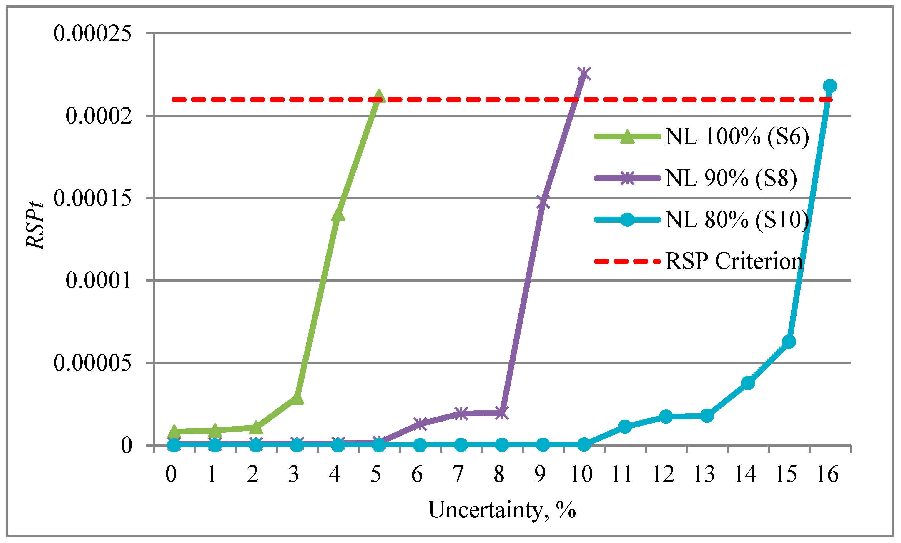
4.2. Results for the Scenarios

Figure 7 represents the result of the sensitivity analysis of the increased variability. The RSPt values differ with the level of the net load; the largest RSPt appears at the highest level of net load, i.e., S1. The largest difference in RSPt according to the net load is between S5 (i.e., the net load is 100%) and S3 (i.e., the net load is 110%) when the increased variability is 18%. In S7 and S9, the values of RSPt are almost unchanged with the uncertainty compared to the other scenarios. In the other scenarios, RSPt increases in a step-wise fashion. This may be related to the failure cases of the generating units.
Figure 8 shows the results of the sensitivity analysis for uncertainty. As in the case of increased variability, RSPt is heavily influenced by the net load. The largest value of RSPt is found when the level of the net load is highest (i.e., S2). S2 (i.e., 120% of the net load) and S4 (i.e., 110% of the net load), when the uncertainty is 4%, make the largest difference in RSPt. In most scenarios, the value of RSPt does not increase much further after it increases sharply. This is related to the characteristics of the probability distribution of the uncertainty, which is modeled as a normal random variable. The left and right sides of the normal distribution are symmetrical with respect to its average, and an increase in the left side (right side) decreases (increases) the RSPt at the same rate. The effects of both sides on the value of RSPt cancel each other out.
When comparing S1, S3, and S5 with S2, S4, and S6, respectively, the values of RSPt and the maximum increments (i.e., the change in the RSPt divided by the change in the uncertainty) in the former scenarios (i.e., S1, S3, and S5) are greater than those in the latter scenarios (i.e., S2, S4, and S6). S7 and S9 are compared to S8 and S10, respectively. The maximum increments in S8 and S10 are greater than those in S7 and S9. The value of RSPt in S8 (S10) is larger than that in S7 (S9) from 10% (12%) to 21% for each parameter. Regarding flexibility, increased variability is more effective than uncertainty when the level of the net load is equal to or greater than 100% (i.e., high and medium types). For the low type, uncertainty is more influential in terms of the maximum increment; however, the more influential parameter in terms of RSPt differs by section.
If the RSPt criterion is set the same as the value of RSPt of the given system (i.e., 2.0982 × 10 4 ), the allowed ranges of increased variability and uncertainty are then determined as shown in Table 3. S1, S2, S3, S4, and S5 do not have allowed ranges under the given conditions, while S6, S7, S8, S9, and S10 have allowed ranges. For reference, Figure 9 and Figure 10 represent the enlarged graphs of Figure 7 and Figure 8, respectively. On the graphs, each point having the value of RSPt smaller than the RSPt criterion is included in the allowed ranges.

5. Conclusions

This study investigated the impact of variability and uncertainty on flexibility. The effects of variability and uncertainty were captured using a flexibility index called the RSP. A case study for a modified IEEE-RTS-96 was performed for a range of variability and uncertainty scenarios, while the level of penetration of renewable energy resources was maintained at the same ratio for every scenario. The simulation results showed that the variability was more effective than the uncertainty, for high and medium net loads. For the low net loads, the more influential parameter depended on the section. The results may differ with the system and its conditions; however, the proposed method can provide system operator with quantified information of the impact of variability and uncertainty for more efficient operation and planning of a power system. As part of future work, it would be interesting to analyze the impact of various strategies enhancing demand flexibility.

Funding

This research was funded by Joongbu University Research & Development Fund.

Conflicts of Interest

The author declares no conflict of interest.

Nomenclature

Ai,tRandom variable representing availability of generator i at time t (1 if available, 0 otherwise)
cElement of Ct−Δt
Ct-ΔtSet of combinations of Ai,t−Δt when Oi,t−Δt is nonzero for all i
eElement of Et
EtSet of NLFEt
FLtForecast load at time t
FNLtForecast net load at time t
FVGtForecast variable generation at time t
iIndex of generator
ISet of generators
LFEtRandom variable representing load forecast error at time t
NLFEtRandom variable representing net load forecast error at time t
Oi,tValue representing whether generator i is online at time t or not
Pi,t Output of generator i at time t
Pmax,iMaximum output level of generator i
Prob(·)Probability in parentheses
Probc[·]Probability of c if condition [∙] is satisfied, 0 otherwise.
RCRtRamping capability requirement at time t
rriRamp rate of generator i
RSPtRamping capability shortage probability at time t
SRCtSystem ramping capability at time t
tIndex of time
ΔtMinimum interval between operating points
VGFEtRandom variable representing variable generation forecast error at time t

Appendix A. Failure and Repair Rates in Case Study

Table A1. Failure and repair rates of 26 generating units.
Unit #Failure Rate (occurrences/h)Repair Rate (occurrences/h)
1–51/29401/60
6–91/4501/50
101/19601/40
11, 121/4501/40
131/19601/40
14–161/12001/50
17–201/9601/40
21–231/9501/50
241/11501/100
25, 261/11001/150

References

  1. The Ministry of Trade, Industry and Energy. The 8th Basic Plan on Electricity Demand and Supply; MOTIE: Sejong-si, Korea, 2017.
  2. Min, C.-G.; Kim, M.-K. Net load carrying capability of generating units in power systems. Energies 2017, 10, 1221. [Google Scholar] [CrossRef]
  3. Min, C.-G.; Kim, M.-K. Flexibility-based reserve scheduling of pumped hydroelectric energy storage in korea. Energies 2017, 10, 1478. [Google Scholar]
  4. Cochran, J.; Miller, M.; Zinaman, O.; Milligan, M.; Arent, D.; Palmintier, B.; O’Malley, M.; Mueller, S.; Lannoye, E.; Tuohy, A. Flexibility in 21st Century Power Systems; U.S. National Renewable Energy Laboratory (NREL): Golden, CO, USA, 2012.
  5. Denholm, P.; Hand, M. Grid flexibility and storage required to achieve very high penetration of variable renewable electricity. Energy Policy 2011, 39, 1817–1830. [Google Scholar] [CrossRef]
  6. Min, C.-G.; Kim, M.-K. Flexibility-based evaluation of variable generation acceptability in korean power system. Energies 2017, 10, 825. [Google Scholar] [CrossRef]
  7. Min, C.-G.; Kim, M.-K. Impact of the complementarity between variable generation resources and load on the flexibility of the korean power system. Energies 2017, 10, 1719. [Google Scholar] [CrossRef]
  8. Navid, N.; Rosenwald, G. Market solutions for managing ramp flexibility with high penetration of renewable resource. IEEE Trans. Sustain. Energy 2012, 3, 784–790. [Google Scholar] [CrossRef]
  9. Halamay, D.A.; Brekken, T.K.; Simmons, A.; McArthur, S. Reserve requirement impacts of large-scale integration of wind, solar, and ocean wave power generation. IEEE Trans. Sustain. Energy 2011, 2, 321–328. [Google Scholar] [CrossRef]
  10. Tabone, M.D.; Callaway, D.S. Modeling variability and uncertainty of photovoltaic generation: A hidden state spatial statistical approach. IEEE Trans. Power Syst. 2015, 30, 2965–2973. [Google Scholar] [CrossRef]
  11. Caciotta, M.; Giarnetti, S.; Leccese, F. In Hybrid neural network system for electric load forecasting of telecomunication station. In Proceedings of the XIX IMEKO World Congress Fundamental and Applied Metrology, Lisbon, Portugal, 6–11 September 2009; pp. 657–661. [Google Scholar]
  12. Ilić, S.; Selakov, A.; Vukmirović, S.; Erdeljan, A.; Kulić, F. Short-term load forecasting in large scale electrical utility using artificial neural network. J. Sci. Ind. Res. 2013, 72, 739–745. [Google Scholar]
  13. Ilić, S.A.; Vukmirović, S.M.; Erdeljan, A.M.; Kulić, F.J. Hybrid artificial neural network system for short-term load forecasting. Therm. Sci. 2012, 16, 215–224. [Google Scholar] [CrossRef]
  14. Kurbatsky, V.; Tomin, N.; Sidorov, D.; Spiryaev, V. In Electricity prices neural networks forecast using the hilbert-huang transform. In Proceedings of the 9th International Conference on Environment and Electrical Engineering (EEEIC), Prague, Czech Republic, 16–19 May 2010; pp. 381–383. [Google Scholar]
  15. Ueckerdt, F.; Brecha, R.; Luderer, G. Analyzing major challenges of wind and solar variability in power systems. Renew. Eenergy 2015, 81, 1–10. [Google Scholar] [CrossRef]
  16. Kiviluoma, J.; Meibom, P.; Tuohy, A.; Troy, N.; Milligan, M.; Lange, B.; Gibescu, M.; O’Malley, M. Short-term energy balancing with increasing levels of wind energy. IEEE Trans. Sustain. Energy 2012, 3, 769–776. [Google Scholar] [CrossRef]
  17. Wang, B.; Liu, X.; Zhu, F.; Hu, X.; Ji, W.; Yang, S.; Wang, K.; Feng, S. Unit commitment model considering flexible scheduling of demand response for high wind integration. Energies 2015, 8, 13688–13709. [Google Scholar] [CrossRef]
  18. Han, X.; Liao, S.; Ai, X.; Yao, W.; Wen, J. Determining the minimal power capacity of energy storage to accommodate renewable generation. Energies 2017, 10, 468. [Google Scholar] [CrossRef]
  19. Jiang, R.; Wang, J.; Guan, Y. Robust unit commitment with wind power and pumped storage hydro. IEEE Trans. Power Syst. 2012, 27, 800. [Google Scholar] [CrossRef]
  20. Bessa, R.; Moreira, C.; Silva, B.; Matos, M. Handling renewable energy variability and uncertainty in power systems operation. Wires Energy Environ. 2014, 3, 156–178. [Google Scholar] [CrossRef]
  21. Osório, G.J.; Shafie-khah, M.; Lujano-Rojas, J.M.; Catalão, J.P. Scheduling model for renewable energy sources integration in an insular power system. Energies 2018, 11, 144. [Google Scholar] [CrossRef]
  22. Marneris, I.G.; Biskas, P.N.; Bakirtzis, A.G. Stochastic and deterministic unit commitment considering uncertainty and variability reserves for high renewable integration. Energies 2017, 10, 140. [Google Scholar] [CrossRef]
  23. Ma, X.-Y.; Sun, Y.-Z.; Fang, H.-L. Scenario generation of wind power based on statistical uncertainty and variability. IEEE Trans. Sustain. Energy 2013, 4, 894–904. [Google Scholar] [CrossRef]
  24. Hu, B.; Wu, L.; Marwali, M. On the robust solution to scuc with load and wind uncertainty correlations. IEEE Trans. Power Syst. 2014, 29, 2952–2964. [Google Scholar] [CrossRef]
  25. Qadrdan, M.; Wu, J.; Jenkins, N.; Ekanayake, J. Operating strategies for a gb integrated gas and electricity network considering the uncertainty in wind power forecasts. IEEE Trans. Sustain. Energy 2014, 5, 128–138. [Google Scholar] [CrossRef]
  26. Ela, E.; O’Malley, M. Studying the variability and uncertainty impacts of variable generation at multiple timescales. IEEE Trans. Power Syst. 2012, 27, 1324. [Google Scholar] [CrossRef]
  27. Weng, Z.; Shi, L.; Xu, Z.; Lu, Q.; Yao, L.; Ni, Y. Fuzzy power flow solution considering wind power variability and uncertainty. Int. Trans. Electr. Energy Syst. 2015, 25, 547–572. [Google Scholar] [CrossRef]
  28. Luo, J.; Shi, L.; Ni, Y. A solution of optimal power flow incorporating wind generation and power grid uncertainties. IEEE Access 2018, 6, 19681–19690. [Google Scholar] [CrossRef]
  29. Min, C.-G.; Park, J.K.; Hur, D.; Kim, M.-K. A risk evaluation method for ramping capability shortage in power systems. Energy 2016, 113, 1316–1324. [Google Scholar] [CrossRef]
  30. Allan, R.N. Reliability Evaluation of Power Systems; Springer Science & Business Media: Berlin, Germany, 2013. [Google Scholar]
  31. Solomon, A.; Kammen, D.M.; Callaway, D. Investigating the impact of wind–solar complementarities on energy storage requirement and the corresponding supply reliability criteria. Appl. Energ. 2016, 168, 130–145. [Google Scholar] [CrossRef]
  32. Borges, C.L.T. An overview of reliability models and methods for distribution systems with renewable energy distributed generation. Renew. Sustain. Energy Rev. 2012, 16, 4008–4015. [Google Scholar] [CrossRef]
  33. Hunt, B.R.; Lipsman, R.L.; Rosenberg, J.M. A Guide to Matlab: For Beginners and Experienced Users; Cambridge University Press: Cambridge, UK, 2014. [Google Scholar]
  34. Korea Power Exchange. Electric Power Statistics Information System. Available online: http://epsis.kpx.or.kr/epsis/ekesStaticMain.do?cmd=001001&flag=&locale=EN (accessed on 17 December 2018).
Figure 1. Triangular distribution for the example.
Applsci 09 00561 g001
Figure 2. Forecast net load variation and measured net load variation.
Applsci 09 00561 g002
Figure 3. Process of scenario generation and sensitivity analysis.
Applsci 09 00561 g003
Figure 4. Forecast net load profile.
Applsci 09 00561 g004
Figure 5. NLFEt and VGFEt distribution. A normal distribution was described using a seven-step approximation.
Applsci 09 00561 g005
Figure 6. Hourly RSPt.
Applsci 09 00561 g006
Figure 7. Results of sensitivity analysis for increased variability.
Applsci 09 00561 g007
Figure 8. Results of sensitivity analysis for uncertainty.
Applsci 09 00561 g008
Figure 9. Results of sensitivity analysis for increased variability: enlarged graph for S7, S9, and RSP criterion.
Applsci 09 00561 g009
Figure 10. Results of sensitivity analysis for uncertainty: enlarged graph for S6, S8, S10, and RSP criterion.
Applsci 09 00561 g010
Table 1. Scenarios for three parameters at the selected time interval.
Scenario #Net LoadIncreased VariabilityUncertainty
S1High (>100%)Particular rangeFixed
S2 Fixed, 0%Particular range
S3Medium (100%)Particular rangeFixed
S4 Fixed, 0%Particular range
S5Low (<100%)Particular rangeFixed
S6 Fixed, 0%Particular range
Table 2. Scenarios for three parameters: net load, increased variability, and uncertainty.
Scenario, S#Net LoadIncreased Variability of the Net Load at 19 hUncertainty of the Net Load at 19 h
S1120%0% to 20%Fixed, i.e., 5%
S2120%Fixed, 0%0% to 20%
S3110%0% to 20%Fixed, i.e., 5%
S4110%Fixed, 0%0% to 20%
S5100%0% to 20%Fixed, i.e., 5%
S6100%Fixed, 0%0% to 20%
S790%0% to 20%Fixed, i.e., 5%
S890%Fixed, 0%0% to 20%
S980%0% to 20%Fixed, i.e., 5%
S1080%Fixed, 0%0% to 20%
Table 3. Allowed ranges of increased variability and uncertainty. ※N/A: not allowed.
Scenario, S#Net LoadIncreased Variability of the Net Load at 19 hUncertainty of the Net Load at 19 h
S1120%N/AFixed, i.e., 5%
S2120%Fixed, 0%N/A
S3110%N/AFixed, i.e., 5%
S4110%Fixed, 0%N/A
S5100%N/AFixed, i.e., 5%
S6100%Fixed, 0%0% to 5%
S790%0% to 11%Fixed, i.e., 5%
S890%Fixed, 0%0% to 10%
S980%0% to 20%Fixed, i.e., 5%
S1080%Fixed, 0%0% to 15%

