Article

Determining the Variability of the Territorial Sea Baseline on the Example of Waterbody Adjacent to the Municipal Beach in Gdynia

1
Department of Transport and Logistics, Gdynia Maritime University, Morska 81-87, 81-225 Gdynia, Poland
2
Department of Geodesy and Oceanography, Gdynia Maritime University, Morska 81-87, 81-225 Gdynia, Poland
3
Institute of Navigation and Hydrography, Polish Naval Academy, Śmidowicza 69, 81-127 Gdynia, Poland
*
Author to whom correspondence should be addressed.
Appl. Sci. 2019, 9(18), 3867; https://doi.org/10.3390/app9183867
Submission received: 3 August 2019 / Revised: 9 September 2019 / Accepted: 10 September 2019 / Published: 14 September 2019
(This article belongs to the Special Issue GNSS Techniques for Land and Structure Monitoring)

Abstract

:
The purpose of this publication is to analyze the spatial and temporal variability of the territorial sea baseline in sand bottom waterbodies, which were determined twice, in 2016 and 2018, by the Real Time Kinematic (RTK) method. This involves direct measurement of sea bottom coordinates on planned hydrographic sounding profiles using a Global Navigation Satellite System (GNSS) receiver mounted on a pole. The data were the basis for creating Digital Terrain Models (DTM), which were then used to determine the baseline for both measurement campaigns. Subsequently, terrain surface models were compared to determine bathymetry changes in the area under analysis, and an assessment was made of the baseline spatial position change over the previous two years. The measurements have shown considerable spatial and temporal variability of the baseline course along a short section of sandy beach. The territorial sea baseline was very unstable; in some places, it moved by even 20–25 m, landwards and seawards. Therefore, one can suppose that these changes are periodic, and one can conclude that the reliability of the baseline measurements can decrease quite quickly.

1. Introduction

Maritime delimitation is an international legal concept which denotes establishing a boundary between states. Regarding maritime areas, a state can determine four types of zones: contiguous zone, continental shelf, exclusive economic zone, and territorial sea [1,2]. Only the territorial sea baseline, which serves as the limit from where the maritime zones are measured, will be analyzed in this paper.
The territorial sea is part of the sovereign territory of the state. It is a belt of coastal waters extending at 12 Nautical Miles (NM) from the baseline (Figure 1) [3,4]. In international regulations related to the maritime industry, two types of baselines are found. The first is a normal baseline, defined as: … “the low-water line along the coast as marked on large-scale charts officially recognized by the coastal state” [4]. With reference to the Article 5 of the United Nations Convention on the Law of the Sea (UNCLOS), the term “coastline” should be understood as the line where land meets the water. Therefore, the normal baseline is coincident to the coastline (low-water line) as portrayed on the charts officially recognized by the states concerned. The fact that this line is almost always under water makes hydrographic surveys necessary for the accurate determination of the low-water line (hence the normal baseline) [5]. This line is used where the coast is regular. The second is a straight baseline which can be applied: … “In localities where the coastline is deeply indented and cut into, or if there is a fringe of islands along the coast in its immediate vicinity” … “Where because of the presence of a delta and other natural conditions the coastline is highly unstable” [4].
It is necessary to determine the baseline mathematically in order to establish the outer limit of the territorial sea, which is the state boundary [7,8,9]. Its determination mainly affects the establishment of the range of sovereign rights of individual states. In the case of Poland, the baseline determination can be considered in the following issues: legal and measurement-related [10,11,12].
In a legal sense, the outer limit of Poland’s territorial sea is established by the domestic legal acts presented in [6]. In view of the dates of these documents (1957–1995) [13] and the variability of the hydrological conditions of the Baltic Sea, it should be stated that Poland currently does not have an actual geographical data set defining the maritime state boundary.
The other issue concerns the methodology of hydrographic measurements on ultra-shallow waters (of the depth below 1 m), i.e., where the baseline is situated [14]. No international standard defines a method of baseline determination, but minimal quality requirements for such measurements are set out in the International Hydrographic Organization (IHO) S-44 standard [15]. Therefore, for many years, baseline measurements have been performed with tachymetric methods [16], satellite methods [17,18], and direct measurements conducted by surveyors on sounding profiles in seawater [19,20]. Over the last dozen or so years, high-resolution satellite images [21,22], Light Detection and Ranging (LiDAR) systems [23], or even Unmanned Surface Vessels (USV) [24,25] have been used to determine the course of the territorial sea baseline.
The purpose of this publication is to analyze the variability of the territorial sea baseline determined twice—in 2016 and 2018—with a geodetic method using a Global Navigation Satellite System (GNSS) receiver on the example of a waterbody adjacent to the municipal beach in Gdynia.

2. Materials and Methods

2.1. Planning Measurement Work

The baseline measurements were carried out in the waterbody adjacent to the municipal beach in Gdynia, which is located in the Bay of Gdańsk. This area is characterized by a typical coastline (straight line sandy section), reinforced with tetrapods and concrete wharves. This is an area with small hydromorphological changes because it is located inside the Bay of Gdańsk, and in its immediate vicinity there is no river mouth that could cause significant changes in the shape of the seafloor. Furthermore, based on long-term research conducted at 35 gauging stations along the Baltic Sea [26], it appears that it is a non-tidal sea because the differences in water levels due to the impact of the tides are small. The minimum tide stood at 3.5 cm at the eastern part of the Bay of Gdańsk (Baltiysk), near the place where the baseline measurements were made.
This research was performed on 23.06.2016 between 08:30 and 18:00, as well as on 19.07.2018 between 11:00 and 14:00. Meteorological conditions that prevailed during the measurements were beneficial, i.e., there was no rain, and the wind did not blow. In order to determine them, short-term weather forecasts were used, which are available on the website: http://www.pogodynka.pl/.
Before research started, the sounding profiles were planned, along which the operator performing the measurement with a GNSS receiver mounted on a pole was supposed to move. Forty main sounding profiles were determined perpendicularly to the shape of the coastline, and the distance between them was 10 m (Figure 2) [27]. The profiles were divided into four sections perpendicularly to the coastline because of the non-linear course of the coast. The above described parallel line method is a common practice used in hydrography because it allows coverage of the entire area with the same accuracy [28,29].
In order to determine territorial sea baseline (according to the Article 5 of UNCLOS Convention), it is necessary to assess the low-water line along the coast as marked on large-scale charts officially recognized by the coastal state [4]. In geographical areas where the tidal range is negligible (for example less than 30 cm) and in non-tidal areas, such as the waterbody adjacent to the municipal beach in Gdynia, the low-water line should be referred to Mean Sea Level (MSL) or another level as closely equivalent to this as is practical and acceptable to Hydrographic Offices [30]. For the purpose of this publication, the low-water line was acquired from the gauging station in the Gdynia marina, situated 200 meters from the measurement site. The minimum water level at the site amounted to 415 cm (on 04.11.1979) and it was referred to the sea level in Kronstadt.
The baseline depth at the measurement time is determined by recording the water level readings. For this purpose, the Institute of Meteorology and Water Management (IMGW-PIB) weather service was used, which provides information on the water levels based on mareograph readings. Under the regulation [31], water levels in Poland can be referred to the Kronstadt vertical coordinate system (PL-KRON86-NH), until 2019, and then to Amsterdam (PL-EVRF2007-NH). The required water level can be determined using the height transformation between the systems PL-EVRF2007-NH and PL-KRON86-NH [32,33]:
H P L K R O N 86 N H = H P L E V R F 2007 N H d H ,
where:
  • HPL-KRON86-NH—normal height of a point in the PL-KRON86-NH system [m],
  • HPL-EVRF2007-NH—normal height of a point in the PL-EVRF2007-NH system [m],
  • dH—difference of normal heights between the systems PL-EVRF2007-NH and PL-KRON86-NH, which depends on the geodetic latitude (ϕ) and longitude (λ) of a point [m].

2.2. Measurements of the Territorial Sea Baseline

Two measurement campaigns were performed in 2016 and 2018; their purpose was to determine the territorial sea baseline by the geodetic method with a GNSS receiver [34,35]. This research involved an operator conducting the measurement on the submerged beach at predefined depth (Figure 3a). During the first measurement campaign on 23.06.2016, the measurements of the seafloor relief were performed at the following depths: 0 (land-water interface), 20, 40, 60, 79 (baseline), 100 cm. The bathymetric measurements of the waterbody during the second campaign were conducted in a similar manner as in the first series. The gauging station at the site in Gdynia showed 494 cm (on 23.06.2016) and 511 cm (on 19.07.2018) relative to the zero ordinate for gauging station in Kronstadt. These data were the basis for calculating the baseline depth (dTSB) from the following formula:
d T S B = H C W L H L W L ,
where:
  • HCWL—current water level in the adopted reference frame [m],
  • HLWL—the lowest water level in the adopted reference frame [m].
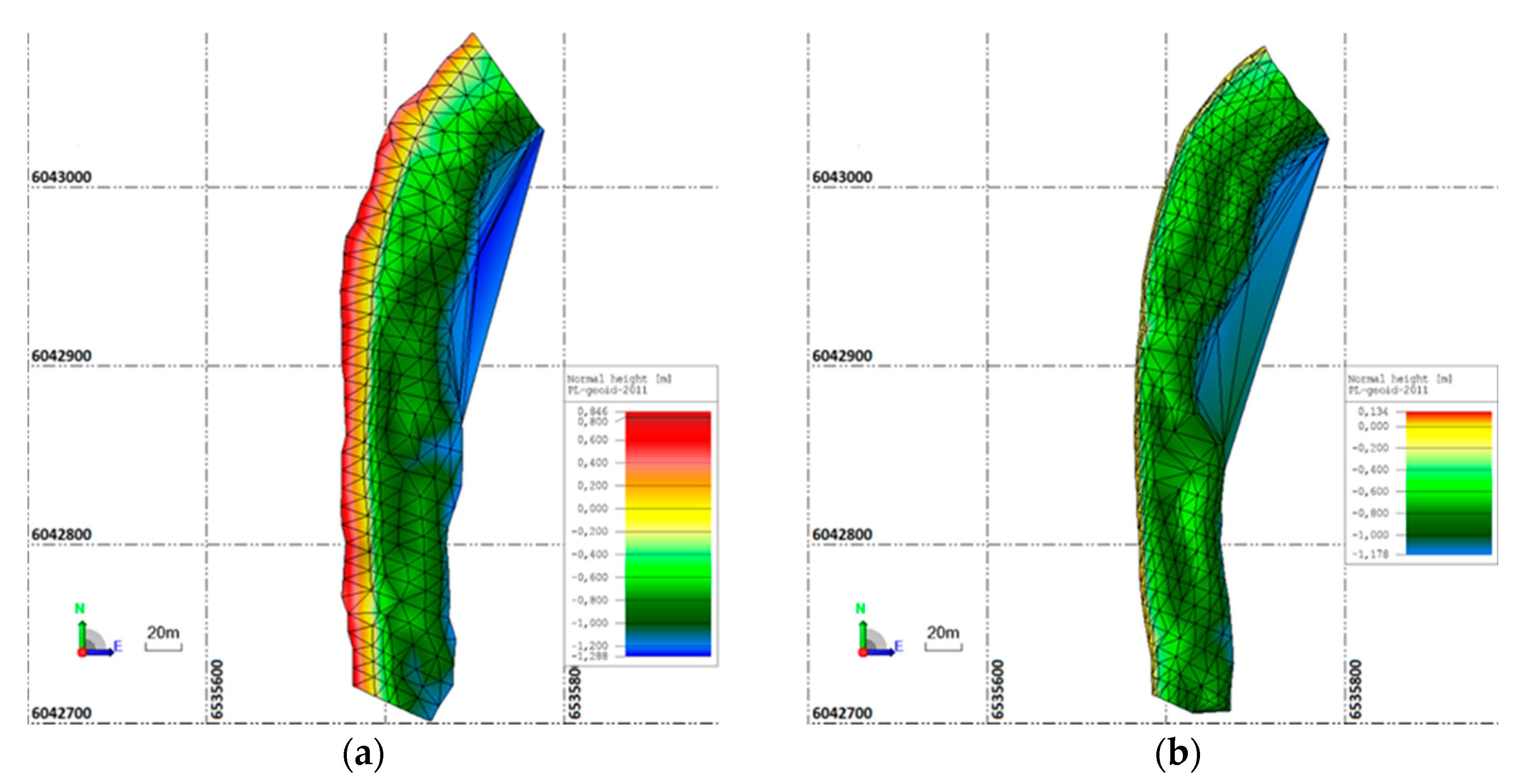
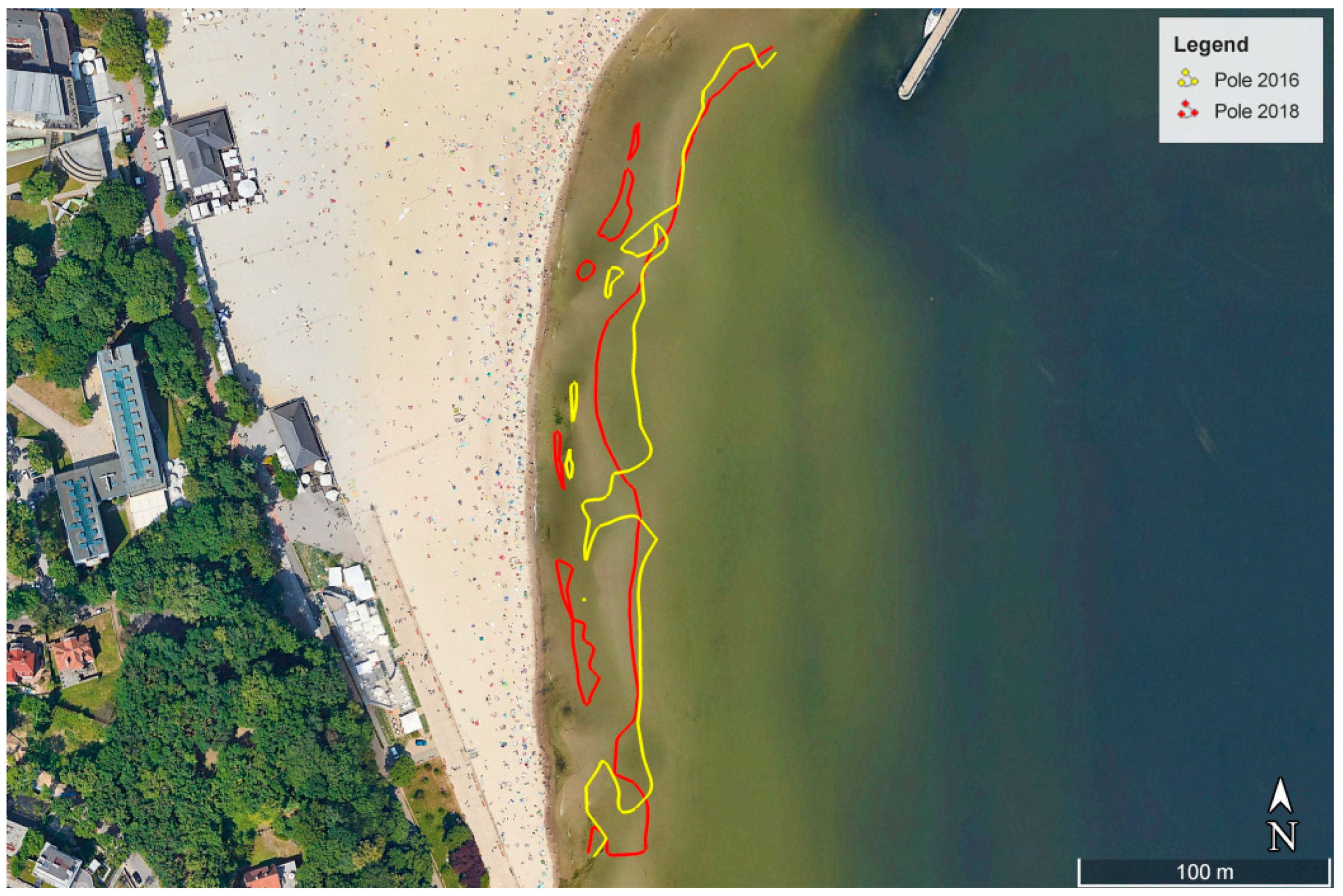
The baseline measurements were conducted on 40 sounding profiles planned during the 2016 measurement campaign [20,36]. Since, during the first test series, the operator performing the baseline measurements along the 400 m long section of the beach was doing it for nearly 10 hours, it was decided that the research in the second measurement campaign could be accelerated by increasing the number of team to two members. Two types of GNSS receivers were used in the research: Leica GS15 and Trimble R10. They made it possible to carry out measurements by the Real Time Kinematic (RTK) method, which provides national GNSS geodetic networks (Leica and VRSNet.pl). Thanks to these services, the data were made with the highest possible positioning accuracy of 1–2 cm (Root Mean Square (RMS)). During the first campaign, 313 points were recorded, and 477 during the second (Figure 3b).
At completion of the measurement, the results were processed with Trimble Business Center (TBC) commercial survey software.

3. Results

During measurement, data processing systems were used: Gauss-Krüger projection, Cartesian coordinate system 2000, height system Kronstadt 86, and the quasigeoid model PL-geoid2011 (Table 1).
Digital Terrain Models (DTM) were developed based on 2016 and 2018 measurement data as Triangulated Irregular Networks (TIN) (Figure 4). A TIN model is created as a result of the triangulation of depth points meeting the Delaunay condition, according to which, a circle determined by three vertices of a triangle cannot contain other depth points, with the exception of degeneracy [37]. Triangle vertices are points of known coordinates. Delaunay triangulation is the dual graph of the Voronoi diagram which has the following property: the distance between each point situated inside a polygon and the nodal point, which is the triangle vertex in the next processing stage, is the shortest [38,39,40]. It should be remembered that in the TIN method, the high-resolution of the generated DTM model is extremely important. As shown by other studies, the TIN method is more accurate only when the points that were used to generate the DTM model are more concentrated [41,42,43].
In order to analyze changes in bathymetry, a height grid with the basic square of 1 × 1 m (maximum available resolution) was created based on DTM models. It can be used to compare the normal height (H) of a point during the past two years. The height grid was created using a tool for creating surfaces and height grid, which is available in the TBC software. This function uses the generated DTM model as the base for height interpolation of the point P in the terrain surface, whose projection P’ on a horizontal plane lies within triangle A’B’C’ (Figure 5).
The height of the point P is calculated from the formula [44]:
H P = H A S A + H B S B + H C S C S A + S B + S C ,
where:
  • HA, HB, HC – normal heights of the triangle ABC,
  • SA, SB, SC – areas of the opposite triangles, formed by division of the triangle A’B’C’ with line segments connecting the triangle vertices with point P’.
Heron’s formula was used to determine the triangle areas (SA, SB, SC). It is used to calculate a triangle area when the lengths of its sides are known. Since the vertex coordinates for the ABC triangle and the rectangular coordinates for point P are given, they can be used to calculate the areas of component triangles. Heron’s formula can be noted in the following manner:
p = a + b + c 2 ,
S = p ( p a ) ( p b ) ( p c ) ,
where:
  • p – semi-perimeter of the A’B’C’ triangle,
  • a, b, c – lengths of sides of the A’B’C’ triangle.
Creating the height grid resulted in 25244 points for the 2016 model and 21561 points for the 2018 model, which were further used to calculate normal height differences at the same points (ΔH2018-2016). In order to determine the spatial and temporal variability of seafloor relief of the waterbody, only those pairs of points were compared (with the same rectangular coordinates on both DTMs) for which normal heights could be calculated. There were 21322 such pairs of points in the area under study.
In the next stage, a DTM model was created (again using the triangulation model) showing differences in normal heights between points with the same rectangular coordinates (X2000, Y2000). The following formula was used to calculate ΔH2018-2016:
Δ H 2018 2016 = H 2018 H 2016 ,
where:
  • H2016, H2018 – normal heights of a point on DTMs based on data acquired by the geodetic method in 2016 and 2018, respectively.
After the height differences between DTM models were generated, a tool for creating contour line, available in the TBC software, was used to mark curves at the following depths: −60 cm, −40 cm, −20 cm, 0 cm, 20 cm, 40 cm (Figure 6). The software generated them as smooth curves using the spline method.
These data show that the greatest bottom variability in the waterbody adjacent to the municipal beach in Gdynia is observed along the coastline. Differences between normal heights range from –60 to –20 cm (Figure 6). Since the normal heights acquired by the geodetic method in 2016 were subtracted from those measured in 2018, it appears that the coastline moved landwards, which resulted in a decrease in the area of the municipal beach in Gdynia. However, when it comes to the remaining part of the waterbody (not directly adjacent to the coastline), one can see that the variability of the seafloor relief in this area is diversed and ranges from –30 cm to 30 cm, regardless of the distance from the coastline. In order to perform an analysis of bathymetry changes, the waterbody was divided into 12 areas according to height differences every 10 cm (Table 2).
Table 2 shows that for nearly 2/3 of the terrain area (64.53%), the height changed only slightly (not more than 20 cm), and for nearly 90%, not more than 30 cm. Changes in the normal heights in the remaining waterbody part (11.3% of the total area) were greater than 30 cm, with the majority of this area being situated along the coast. Apart from the division of the waterbody area with respect to height differences between DTMs, an analysis of changes of its volume was also performed (Table 3).
Table 3 shows that the sand volume increased by 1695.2 m3 and decreased by 759.1 m3 in the area of 21070.7 m2 (the municipal beach in Gdynia has a sandy bottom) within the past two years. The landmass balance, i.e., the difference between the total erosion volume (VTE) and the total accretion volume (VTA) shows that the sand volume in the area increased by 936.1 m3. This amount is relatively small because if the excess sand was spread evenly across the entire area, the bottom of the waterbody adjacent to the municipal beach in Gdynia would increase by just 4 cm.
The analyzes also included an assessment of the territorial sea baseline variability within the past two years. The distance between the baseline and the coastline was adopted as the measure of changes of the territorial sea baseline. Since the coastline moved landwards by several meters during the period under analysis, the reference line was determined first, and it was used as the basis to calculate the distance to the baselines. To do this, the coordinates of points measured along the coastline in 2016 and 2018 were used. Subsequently, the data were used to calculate the linear regression coefficients (for the reference line) by the least-squares method from the following formulas [45,46]:
b = ( X C Y C ) N C X ¯ C Y ¯ C Y C 2 N C Y ¯ C 2 ,
a = X ¯ C b Y ¯ C ,
where:
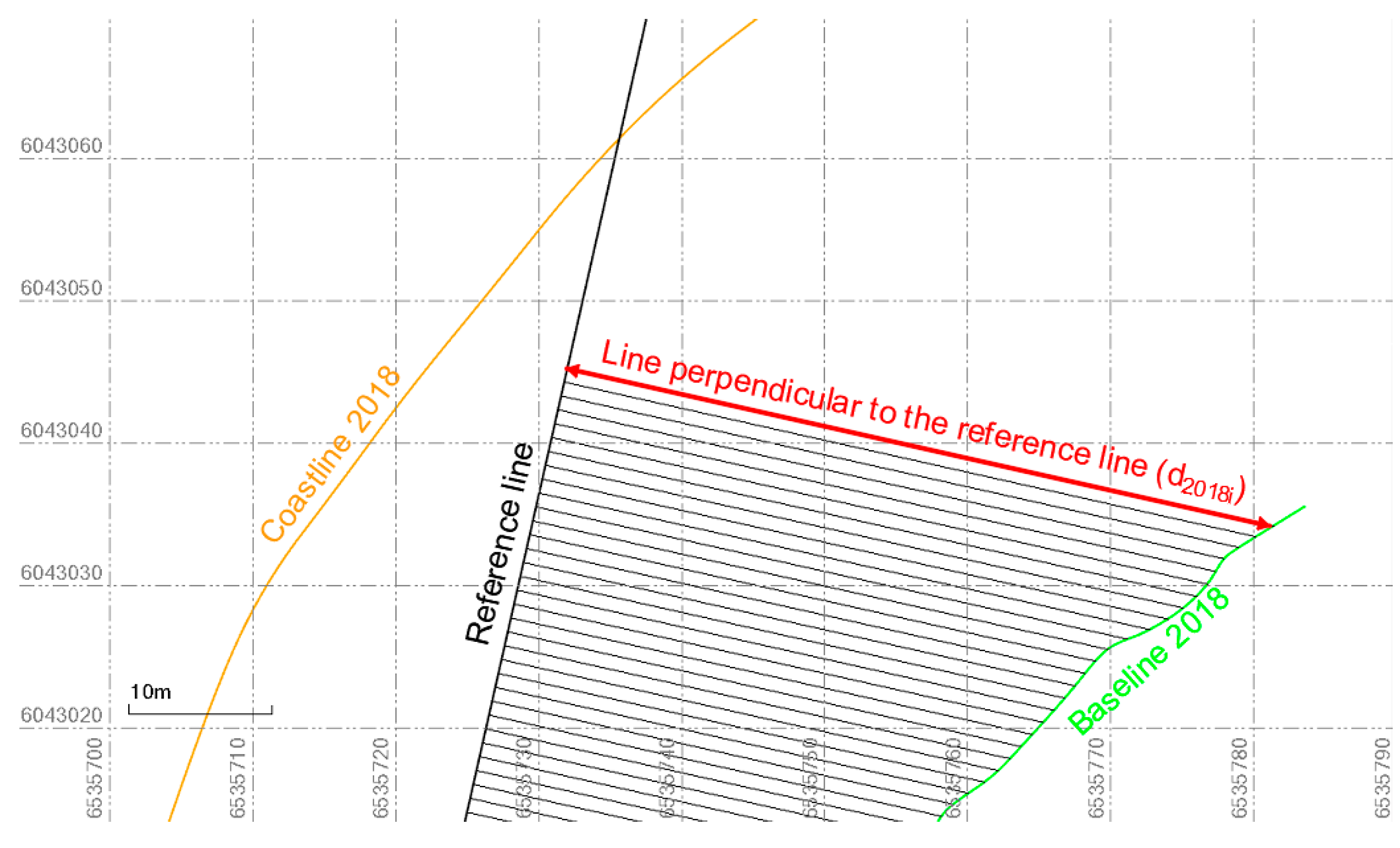
  • XC, YC—rectangular coordinates PL-2000 of the points measured along the coastline in 2016 and 2018,
  • NC—the number of points measured along the coastline in 2016 and 2018,
  • X ¯ C —arithmetic average for the northing coordinates of points measured along the coastline in 2016 and 2018,
  • Y ¯ C —arithmetic average for the easting coordinates of points measured along the coastline in 2016 and 2018.
The reference line has the following form:
X R L = b Y R L + a ,
where:
  • XRL, YRL —rectangular coordinates PL-2000 of the points that determine the reference line.
After the reference line was determined, the distances between the approximate line and the baselines were calculated. Lines perpendicular to the reference line were drawn; they can be described by the formula:
X P L i = 1 b Y P L i + a i ,
where:
  • XPLi, YPLi – rectangular coordinates PL-2000 of the points that determine the i-th line perpendicular to the reference line,
  • i – numbering of perpendicular lines, increasing southwards.
The formula (10) does not provide the numerical value of parameter ai because it depends on the distance between successive perpendicular lines. It was assumed for this study that the distance will be 1 m.
The distances between the reference line and the baseline (di) were calculated from the coordinates of these lines intersecting with the perpendicular line drawn to the reference line (Figure 7):
d i = ( X R L i X T S B i ) 2 + ( Y R L i Y T S B i ) 2 ,
where:
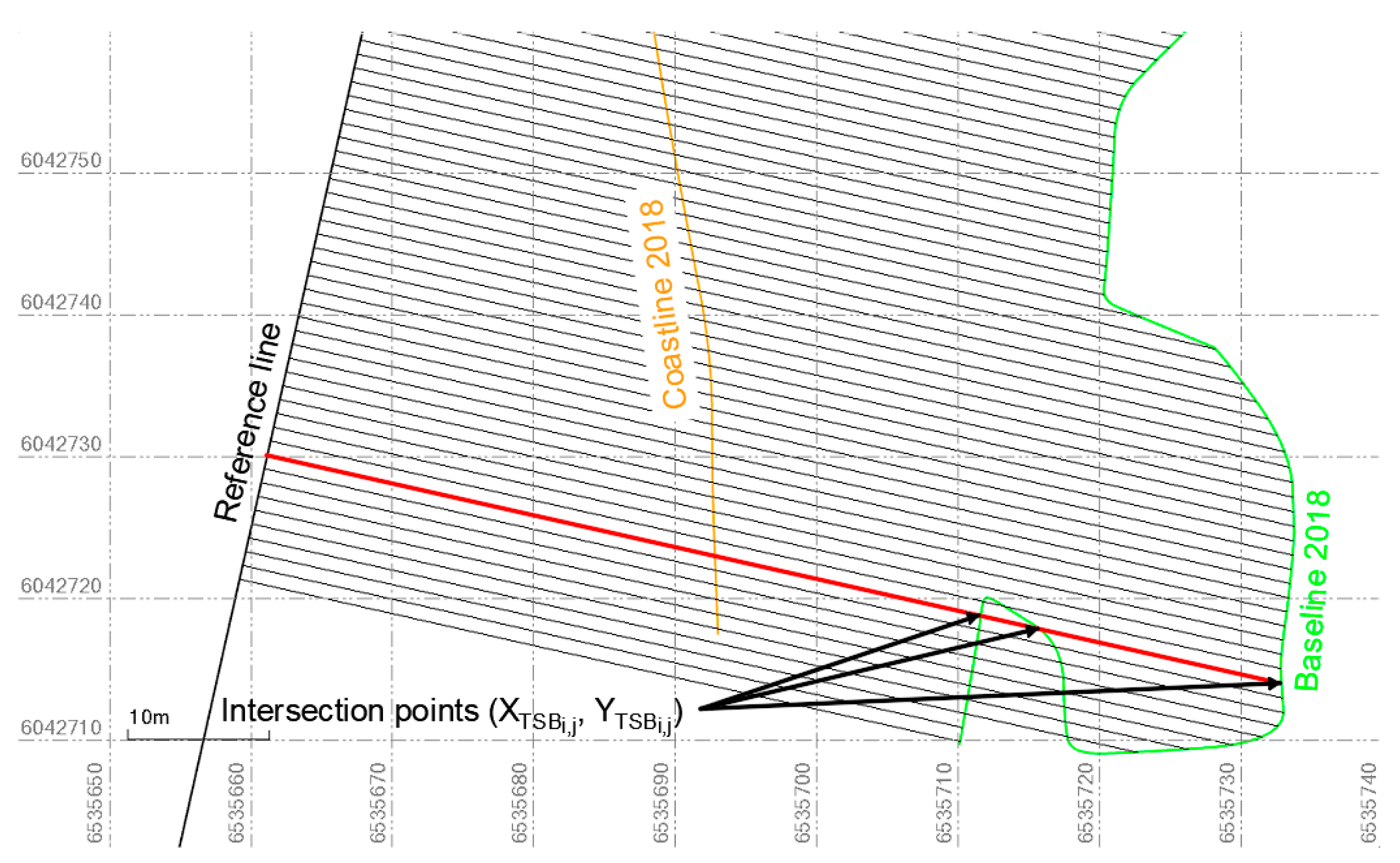
  • XRLi, YRLi—rectangular coordinates PL-2000 of the reference line intersection points with the i-th line perpendicular to it,
  • XTSBi, YTSBi—rectangular coordinates PL-2000 of the baseline intersection points with the i-th line perpendicular to the reference line.
If the perpendicular line intersected the baseline at more than one point (Figure 8), the coordinates of these lines intersection were averaged first ( X ¯ T S B i , Y ¯ T S B i ):
X ¯ T S B i = j = 1 k X T S B i , j k ,
Y ¯ T S B i = j = 1 k Y T S B i , j k ,
where:
  • j—number of the baseline intersection with the i-th line perpendicular to the reference line,
  • k—the number of the baseline intersections with the i-th line perpendicular to the reference line,
and subsequently they were used to calculate the distance to the reference line:
d i = ( X R L i X ¯ T S B i ) 2 + ( Y R L i Y ¯ T S B i ) 2 ,
After calculating the distance between the reference line and the baselines (measured in 2016 and 2018), the spatial and temporal variability of the territorial sea baseline were determined by calculating the distance between the baselines (Δd2018-2016i) using the following formula:
Δ d 2018 2016 i = d 2018 i d 2016 i ,
where:
  • d2016i—distance between the baseline measured in 2016 and the reference line calculated along the i-th line perpendicular to the reference line,
  • d2018i—distance between the baseline measured in 2018 and the reference line calculated along the i-th line perpendicular to the reference line.
In Figure 9, there is presented the changes in the territorial sea baseline course in the waterbody adjacent to the municipal beach in Gdynia over two years.
Figure 9 shows that the spatial and temporal variability of the baseline course is quite large. The largest differences were observed in the middle section of the waterbody, where the territorial sea baseline moved landwards by several meters (coastline chainage: 0.125–0.175 km), and even moved by more than twenty meters into the sea (coastline chainage: 0.2 km). Moreover, considerable differences were noted in the southern part of the waterbody (coastline chainage: 0.325 km) between the baselines, from several to even 25 m.
Statistically, the baseline has changed with a mean variability of 9.50 m over the two-year period of observation. Thus, it can be claimed that the position of the territorial sea baseline along the waterbody is not stable. This statistical measure was calculated from the following formula:
σ Δ d 2018 2016 = i = 1 N ( Δ d 2018 2016 i Δ d ¯ 2018 2016 ) 2 N 1 ,
where:
  • N—the number of lines perpendicular to the reference line.
At the final stage of the work, it was decided to visualize the course of the baselines, which were determined in 2016 and 2018 (Figure 10). To this end, free Google Earth Pro software was used to map the Earth by superimposing satellite images, aerial photography, and Geographic Information System (GIS) data onto a 3D globe.

4. Discussion

The purpose of this publication is to analyze the variability of the territorial sea baseline determined twice, in 2016 and 2018, by a geodetic method using a GNSS receiver in the 400 m long waterbody adjacent to the municipal beach in Gdynia. Apart from that, changes of bathymetry in the area under analysis were determined to verify the study results.
These measurements have shown considerable spatial and temporal variability of the baseline course along a short section of sandy beach. Figure 9 shows that the territorial sea baseline is very unstable because, in some places, it moved by even 20–25 m, landwards and seawards. It is particularly noticeable in the middle section of the waterbody, between the coastline chainage of 0.1 and 0.2 km. Such large variability of the baseline may have been caused by successive “shallows” on several profiles (Figure 10). Between the “shallows” there were “depressions” whose depths corresponded to the baseline. Therefore, one can suppose that these local bottom surface elevations change periodically, and one can conclude that the reliability of the baseline measurements can decrease quite quickly. Statistically, the baseline has changed with a mean variability of 9.50 m over the two-year period of observation. Thus, it can be claimed that the position of the territorial sea baseline along the waterbody is not stable.
Table 3 shows that the sand volume increased by 1695.2 m3 and decreased by 759.1 m3 in the area of 21070.7 m2 (the municipal beach in Gdynia has a sandy bottom) within the past two years. The landmass balance—i.e., the difference between the total erosion volume (VTE) and the total accretion volume (VTA)—shows that the sand volume in the area increased by 936.1 m3. This amount is relatively small because if the excess sand was spread evenly across the entire area, the bottom of the waterbody adjacent to the municipal beach in Gdynia would increase by just 4 cm.
The measured waterbody is adjacent to the Yacht Basin named Mariusz Zaruski in Gdynia, which are approached by vessels with a draft not exceeding 3.20 m. Due to the fact that fine sand is lying on the bottom in this area, this shipping connection may have an impact on the bathymetry changes. North-east and east winds occurring in autumn and winter are another very important hydrometeorological factor; their forces reach even 3–5 on the Beaufort scale. These winds cause the formation of high waves and significant changes in sea levels during this period, which may be up to 1.37 m higher or 0.97 m lower than average. As for the sea currents, in this region along the breakwater, there is a weak north current, which during northern and north-east winds reaches a speed of up to 2 knots [47]. Hence, according to the Authors, the most important hydrometeorological factor that had an impact on bathymetry changes of the waterbody adjacent to the municipal beach in Gdynia and the territorial sea baseline was wind.
The baseline measurements performed by geodetic methods had many limitations, which included low coverage and duration. Therefore, the Authors recommend conducting bathymetric measurements in ultra-shallow waters by the hydrographic method, which involves the use of an unmanned surface vessel (a drone with a dozen centimetre draft) [48,49,50,51,52,53,54,55,56], on which a GNSS receiver and a Single Beam Echo Sounder (SBES) can be mounted. These measurement techniques enable high precision (1–5 cm (p = 0.95)) hydroacoustic surveys [57,58,59,60,61,62,63,64] performed during a relatively short time. However, one must bear in mind that an unmanned surface vessel cannot measure a whole waterbody [24]. It is caused by the following factors: minimum sounding depth (ca. 30 cm) and vessel draft. Hence, the area between the coastline and the 30/40 cm isobath should be measured by the geodetic method [20] or photogrammetric method with unmanned [65] or manned aircraft [66,67]. Moreover, alternatively, the coastal water depths can be determined by analyzing high-resolution satellite images [68,69,70,71].

Author Contributions

Conceptualization, M.S. (Mariusz Specht) and C.S.; Data curation, P.D. and M.S. (Marcin Skóra); Formal analysis, M.S. (Mariusz Specht) and M.W.; Investigation, M.S. (Mariusz Specht), P.D., M.S. (Marcin Skóra) and Ł.M.; Methodology, C.S. and M.W.; Supervision, C.S.; Visualization, M.S. (Mariusz Specht) and Ł.M.; Writing—original draft, M.S. (Mariusz Specht) and M.W.; Writing—review & editing, P.D., M.S. (Marcin Skóra) and Ł.M.

Funding

This research has been financed from the science budget for 2016-20, as a research project within the “Diamentowy Grant” Programme No. DI2015 008545.

Conflicts of Interest

The Authors declare no conflict of interest.

References

  1. Klein, N. Litigating International Law Disputes: Weighing the Options; Cambridge University Press: New York, NY, USA, 2014. [Google Scholar]
  2. Pina-Garcia, F.; Pereda-Garcia, R.; de Luis-Ruiz, J.M.; Perez-Alvarez, R.; Husillos-Rodriguez, R. Determination of geometry and measurement of maritime-terrestrial lines by means of fractals: Application to the Coast of Cantabria (Spain). J. Coast. Res. 2016, 32, 1174–1183. [Google Scholar] [CrossRef]
  3. Hodgson, R.D. Maritime limits and boundaries. Mar. Geod. 1977, 1, 155–163. [Google Scholar] [CrossRef]
  4. United Nations Convention on the Law of the Sea. United Nations Convention on the Law of the Sea of 10 December 1982; UNCLOS: Montego Bay, Jamaica, 1982. [Google Scholar]
  5. Kastrisios, C. Maritime Zones and Boundaries Delimitation Analysis and Implementation in a Digital Environment. Ph.D. Thesis, National Technical University of Athens, Zografou, Greece, 2017. [Google Scholar] [CrossRef]
  6. Ministry of Infrastructure and Development of the Republic of Poland. Justification of the Draft Ordinance of the Council of Ministers on the Detailed Course of the Baseline, External Boundary of the Territorial Sea and the External Boundary of Contiguous Zone of the Republic of Poland. Available online: https://www.senat.gov.pl/download/gfx/senat/pl/senatposiedzeniatematy/2737/drukisejmowe/3661.pdf (accessed on 5 July 2019). (In Polish)
  7. Abidin, H.Z.; Sutisna, S.; Padmasari, T.; Villanueva, K.J.; Kahar, J. Geodetic datum of Indonesian maritime boundaries: Status and problems. Mar. Geod. 2005, 28, 291–304. [Google Scholar] [CrossRef]
  8. Grafarend, E.; Okeke, F. Transformation of lambert conic conformal coordinates from a global datum to a local datum. Mar. Geod. 2007, 30, 297–313. [Google Scholar] [CrossRef]
  9. Horemuz, M. Error calculation in maritime delimitation between states with opposite or adjacent coasts. Mar. Geod. 1999, 22, 1–17. [Google Scholar] [CrossRef]
  10. Kabziński, P.; Weintrit, A. Applications of GIS on issues concerning maritime delimitation. Hydrogr. Rev. 2008, 4, 1–14. (In Polish) [Google Scholar]
  11. Misiak, W.; Felczak, J. Maritime borders and maritime border zones. Sci. Pap. Sil. Univ. Technol. Organ. Manag. Ser. 2013, 65, 237–255. (In Polish) [Google Scholar]
  12. Wolny, B. Geodesy and Cartography in Territorial Sea. Available online: http://www.geodezja-szczecin.org.pl/Grafika/wolny/morze.pdf (accessed on 5 July 2019). (In Polish).
  13. Council of Ministers of the Republic of Poland. Ordinance of the Council of Ministers of 13 January 2017 on the Detailed Course of the Baseline, External Boundary of the Territorial Sea and the External Boundary of Contiguous Zone of the Republic of Poland, 2017; Council of Ministers of the Republic of Poland: Warsaw, Poland, 2017. (In Polish) [Google Scholar]
  14. Specht, M.; Specht, C.; Wąż, M.; Naus, K.; Grządziel, A.; Iwen, D. Methodology for performing territorial sea baseline measurements in selected waterbodies of Poland. Appl. Sci. 2019, 9, 3053. [Google Scholar] [CrossRef]
  15. International Hydrographic Organization. IHO Standards for Hydrographic Surveys, 5th ed.; Special Publication No. 44; IHO: Monte Carlo, Monaco, 2008. [Google Scholar]
  16. Geirr Harsson, B.; Preiss, G. Norwegian baselines, maritime boundaries and the UN convention on the law of the sea. Arct. Rev. Law Politics 2012, 3, 108–129. [Google Scholar]
  17. Cosquer, G.; Hangouet, J.F. Delimitation of land and maritime boundaries: Geodetic and geometric bases. In Proceedings of the FIG Working Week 2003, Paris, France, 13–17 April 2003. [Google Scholar]
  18. Farboud, S. Determination of accurate sea border lines of countries. In Proceedings of the FIG Working Week 2012, Rome, Italy, 6–10 May 2012. [Google Scholar]
  19. Baptista, P.; Bastos, L.; Bernardes, C.; Cunha, T.; Dias, J. Monitoring sandy shores morphologies by DGPS —A practical tool to generate digital elevation models. J. Coast. Res. 2008, 24, 1516–1528. [Google Scholar] [CrossRef]
  20. Specht, C.; Weintrit, A.; Specht, M.; Dąbrowski, P. Determination of the territorial sea baseline—Measurement aspect. IOP Conf. Ser. Earth Environ. Sci. 2017, 95, 1–10. [Google Scholar] [CrossRef]
  21. Markiewicz, Ł.; Mazurek, P.; Chybicki, A. Coastline change-detection method using remote sensing satellite observation data. Hydroacoustics 2016, 19, 277–284. [Google Scholar]
  22. Tang, K.K.W.; Mahmud, M.R.; Hussaini, A.; Abubakar, A.G. An aid in determining the territorial sea baseline using satellite-derived bathymetry. In Proceedings of the FIG Working Week 2019, Hanoi, Vietnam, 22–26 April 2019. [Google Scholar]
  23. Sinclair, M.J.; Stephenson, D.J.; Barker, R.M. Alaska Peninsula deployment of laser airborne bathymetric system. In Proceedings of the Oceans 2003, Celebrating the Past … Teaming Toward the Future, San Diego, CA, USA, 22–26 September 2003. [Google Scholar]
  24. Specht, C.; Specht, M.; Cywiński, P.; Skóra, M.; Marchel, Ł.; Szychowski, P. A new method for determining the territorial sea baseline using an unmanned, hydrographic surface vessel. J. Coast. Res. 2019, 35, 925–936. [Google Scholar] [CrossRef]
  25. Specht, C.; Weintrit, A.; Specht, M. Determination of the territorial sea baseline—Aspect of using unmanned hydrographic vessels. Transnav Int. J. Mar. Navig. Saf. Sea Transp. 2016, 10, 649–654. [Google Scholar] [CrossRef]
  26. Medvedev, I.P.; Rabinovich, A.B.; Kulikov, E.A. Tidal oscillations in the Baltic Sea. Oceanology 2013, 53, 526–538. [Google Scholar] [CrossRef]
  27. Kierzkowski, W. Marine Measurements. Part I. Hydrographic Measurements; Polish Naval Academy Publishing House: Gdynia, Poland, 1984; Volume 1. (In Polish) [Google Scholar]
  28. Sciortino, J.A. Fishing Harbour Planning, Construction and Management; Food and Agriculture Organization of the United Nations: Rome, Italy, 2010. [Google Scholar]
  29. Stenborg, E. The Swedish parallel sounding method state of the art. Int. Hydrogr. Rev. 1987, 64, 7–14. [Google Scholar]
  30. International Hydrographic Organization. Resolutions of the International Hydrographic Organization, Publication M-3, 2nd ed.; IHO: Monte Carlo, Monaco, 2018. [Google Scholar]
  31. Council of Ministers of the Republic of Poland. Ordinance of the Council of Ministers of 15 October 2012 on the National Spatial Reference System; Council of Ministers of the Republic of Poland: Warsaw, Poland, 2012. (In Polish) [Google Scholar]
  32. Kurałowicz, Z.; Słomska, A. Mareographic stations and selected vertical datums in Europe. Mar. Eng. Geotech. 2015, 6, 843–853. (In Polish) [Google Scholar]
  33. Kurałowicz, Z.; Słomska, A. surfaces and vertical reference systems—Observations at mareograph stations in Kronstadt and Amsterdam. Mar. Eng. Geotech. 2014, 5, 377–384. (In Polish) [Google Scholar]
  34. Czaplewski, K.; Specht, C. Determination of coast and base line by GPS techniques. Navig. Hydrogr. 2002, 14, 137–144. [Google Scholar]
  35. Czaplewski, K.; Kołaczyński, S.; Specht, C. The use of GPS system for determining the territorial sea baseline and the coastline of the Republic of Poland. In Proceedings of the 12th International Scientific and Technical Conference “The Role of Navigation in Support of Human Activity at Sea”, Gdynia, Poland, 18–22 April 2000. (In Polish). [Google Scholar]
  36. Specht, M.; Specht, C. Hydrographic survey planning for the determination of territorial sea baseline on the example of selected Polish sea areas. In Proceedings of the 18th International Multidisciplinary Scientific GeoConference SGEM 2018, Albena, Bulgaria, 2–8 July 2018. [Google Scholar] [CrossRef]
  37. Verbree, E. Delaunay tetrahedralizations: Honor degenerated cases. Int. Arch. Photogramm. Remote Sens. Spat. Inf. Sci. 2010, 38-4/W15, 69–72. [Google Scholar]
  38. Jingsheng, Z.; Yi, L. Recognition and measurement of marine topography for sounding generalization in digital nautical chart. Mar. Geod. 2005, 28, 167–174. [Google Scholar] [CrossRef]
  39. Peters, R.; Ledoux, H.; Meijers, M. A Voronoi-based approach to generating depth-contours for hydrographic charts. Mar. Geod. 2014, 37, 145–166. [Google Scholar] [CrossRef]
  40. Sui, H.; Zhu, X.; Zhang, A. A system for fast cartographic sounding selection. Mar. Geod. 2005, 28, 159–165. [Google Scholar] [CrossRef]
  41. Guo, Q.; Li, W.; Yu, H.; Alvarez, O. Effects of topographic variability and lidar sampling density on several DEM interpolation methods. Photogramm. Eng. Remote Sens. 2010, 76, 701–712. [Google Scholar] [CrossRef]
  42. Hu, B.; Gumerov, D.; Wang, J.; Zhang, W. An integrated approach to generating accurate DTM from airborne full-waveform lidar data. Remote Sens. 2017, 9, 871. [Google Scholar] [CrossRef]
  43. Stereńczak, K.; Ciesielski, M.; Balazy, R.; Zawiła-Niedźwiecki, T. Comparison of various algorithms for DTM interpolation from lidar data in dense mountain forests. Eur. J. Remote Sens. 2016, 49, 599–621. [Google Scholar] [CrossRef]
  44. Kendig, K. Is a 2000-year-old formula still keeping some secrets? Am. Math. Mon. 2000, 107, 402–415. [Google Scholar] [CrossRef]
  45. Chatterjee, S.; Hadi, A.S. Regression Analysis by Example, 4th ed.; Wiley: New Yok, NY, USA, 2006. [Google Scholar]
  46. Molugaram, K.; Shanker Rao, G. Analysis of time series. In Statistical Techniques for Transportation Engineering; Elsevier: Amsterdam, The Netherlands, 2017; pp. 463–489. [Google Scholar]
  47. Biuro Hydrograficzne Marynarki Wojennej. Baltic Sea Pilot Book, Polish Coast, 502, 9th ed.; BHMW: Gdynia, Poland, 2009. (In Polish)
  48. Aucelli, P.; Cinque, A.; Mattei, G.; Pappone, G. Historical sea level changes and effects on the coasts of Sorrento Peninsula (Gulf of Naples): New constrains from recent geoarchaeological investigations. Palaeogeogr. Palaeoclimatol. Palaeoecol. 2016, 463, 112–125. [Google Scholar] [CrossRef]
  49. Giordano, F.; Mattei, G.; Parente, C.; Peluso, F.; Santamaria, R. MicroVEGA (Micro Vessel for Geodetics Application): A marine drone for the acquisition of bathymetric data for GIS applications. Int. Arch. Photogramm. Remote Sens. Spat. Inf. Sci. 2015, 40, 123–130. [Google Scholar] [CrossRef]
  50. Kum, B.C.; Shin, D.H.; Lee, J.H.; Moh, T.J.; Jang, S.; Lee, S.Y.; Cho, J.H. Monitoring applications for multifunctional unmanned surface vehicles in marine coastal environments. J. Coast. Res. 2018, 85, 1381–1385. [Google Scholar] [CrossRef]
  51. Liang, J.; Zhang, J.; Ma, Y.; Zhang, C.Y. Derivation of bathymetry from high-resolution optical satellite imagery and USV sounding data. Mar. Geod. 2017, 40, 466–479. [Google Scholar] [CrossRef]
  52. Stateczny, A.; Gierski, W. The concept of anti-collision system of autonomous surface vehicle. E3S Web Conf. 2018, 63, 1–6. [Google Scholar] [CrossRef]
  53. Stateczny, A.; Grońska, D.; Motyl, W. Hydrodron—New step for professional hydrography for restricted waters. In Proceedings of the 2018 Baltic Geodetic Congress, Olsztyn, Poland, 21–23 June 2018. [Google Scholar]
  54. Stateczny, A.; Kazimierski, W.; Burdziakowski, P.; Motyl, W.; Wisniewska, M. Shore construction detection by automotive radar for the needs of autonomous surface vehicle navigation. Int. J. Geo-Inf. 2019, 8, 80. [Google Scholar] [CrossRef]
  55. Stateczny, A.; Włodarczyk-Sielicka, M.; Grońska, D.; Motyl, W. Multibeam echosounder and lidar in process of 360-degree numerical map production for restricted waters with HydroDron. In Proceedings of the 2018 Baltic Geodetic Congress, Olsztyn, Poland, 21–23 June 2018. [Google Scholar]
  56. Suhari, K.T.; Karim, H.; Gunawan, P.H.; Purwanto, H. Small ROV marine boat for bathymetry surveys of shallow waters—Potential implementation in Malaysia. Int. Arch. Photogramm. Remote Sens. Spat. Inf. Sci. 2017, 42, 201–208. [Google Scholar] [CrossRef]
  57. El-Hattab, A.I. Investigating the effects of hydrographic survey uncertainty on dredge quantity estimation. Mar. Geod. 2014, 37, 389–403. [Google Scholar] [CrossRef]
  58. Jang, W.S.; Park, H.S.; Seo, K.Y.; Kim, Y.K. Analysis of positioning accuracy using multi differential GNSS in coast and port area of South Korea. J. Coast. Res. 2016, 75, 1337–1341. [Google Scholar] [CrossRef]
  59. Specht, C.; Koc, W.; Smolarek, L.; Grządziela, A.; Szmagliński, J.; Specht, M. Diagnostics of the tram track shape with the use of the global positioning satellite systems (GPS/GLONASS) measurements with a 20 Hz frequency sampling. J. Vibroengineering 2014, 16, 3076–3085. [Google Scholar]
  60. Specht, C.; Makar, A.; Specht, M. Availability of the GNSS geodetic networks position during the hydrographic surveys in the ports. Transnav Int. J. Mar. Navig. Saf. Sea Transp. 2018, 12, 657–661. [Google Scholar] [CrossRef]
  61. Specht, C.; Pawelski, J.; Smolarek, L.; Specht, M.; Dąbrowski, P. Assessment of the positioning accuracy of DGPS and EGNOS systems in the Bay of Gdansk using maritime dynamic measurements. J. Navig. 2019, 72, 575–587. [Google Scholar] [CrossRef]
  62. Specht, C.; Specht, M.; Dąbrowski, P. Comparative analysis of active geodetic networks in Poland. In Proceedings of the 17th International Multidisciplinary Scientific GeoConference SGEM 2017, Albena, Bulgaria, 27 June–6 July 2017. [Google Scholar] [CrossRef]
  63. Specht, C.; Świtalski, E.; Specht, M. Application of an autonomous/unmanned survey vessel (ASV/USV) in bathymetric measurements. Pol. Marit. Res. 2017, 24, 36–44. [Google Scholar] [CrossRef]
  64. Specht, M. Method of evaluating the positioning system capability for complying with the minimum accuracy requirements for the international hydrographic organization orders. Sensors 2019, 19, 3860. [Google Scholar] [CrossRef]
  65. Albuquerque, M.; Alves, D.C.L.; Espinoza, J.M.A.; Oliveira, U.R.; Simoes, R.S. Determining shoreline response to meteo-oceanographic events using remote sensing and unmanned aerial vehicle (UAV): Case study in Southern Brazil. J. Coast. Res. 2018, 85, 766–770. [Google Scholar] [CrossRef]
  66. Bachmann, C.M.; Montes, M.J.; Fusina, R.A.; Parrish, C.; Sellars, J.; Weidemann, A.; Goode, W.; Nichols, C.R.; Woodward, P.; McIlhany, K.; et al. Bathymetry retrieval from hyperspectral imagery in the very shallow water limit: A case study from the 2007 Virginia Coast Reserve (VCR’07) multi-sensor campaign. Mar. Geod. 2010, 33, 53–75. [Google Scholar] [CrossRef]
  67. Kim, H.; Lee, S.B.; Min, K.S. Shoreline change analysis using airborne lidar bathymetry for coastal monitoring. J. Coast. Res. 2017, 79, 269–273. [Google Scholar] [CrossRef]
  68. Chybicki, A. Three-dimensional geographically weighted inverse regression (3GWR) model for satellite derived bathymetry using Sentinel-2 observations. Mar. Geod. 2018, 41, 1–23. [Google Scholar] [CrossRef]
  69. Hogrefe, K.R.; Wright, D.J.; Hochberg, E.J. Derivation and integration of shallow-water bathymetry: Implications for coastal terrain modeling and subsequent analyzes. Mar. Geod. 2008, 31, 299–317. [Google Scholar] [CrossRef]
  70. Kulawiak, M.; Chybicki, A. Application of Web-GIS and geovisual analytics to monitoring of seabed evolution in South Baltic Sea coastal areas. Mar. Geod. 2018, 41, 405–426. [Google Scholar] [CrossRef]
  71. Warnasuriya, T.W.S.; Gunaalan, K.; Gunasekara, S.S. Google earth: A new resource for shoreline change estimation—Case study from Jaffna Peninsula, Sri Lanka. Mar. Geod. 2018, 41, 1–35. [Google Scholar] [CrossRef]
Figure 1. The effect of the baseline to the outer limits of maritime zones. Own study based on: [6].
Applsci 09 03867 g001
Figure 2. The planning of hydrographic profiles during baseline measurements in Gdynia.
Applsci 09 03867 g002
Figure 3. Territorial sea baseline measurement (a) and recorded measurement points (b) by the geodetic method during the second measurement campaign.
Applsci 09 03867 g003
Figure 4. Digital Terrain Models (DTM) of the waterbody adjacent to the municipal beach in Gdynia acquired by the geodetic method in 2016 (a) and 2018 (b).
Applsci 09 03867 g004
Figure 5. Illustration of point height determination in a Triangulated Irregular Networks (TIN) model.
Applsci 09 03867 g005
Figure 6. Height differences between DTMs created on the basis of data acquired by the geodetic method in 2016 and 2018.
Applsci 09 03867 g006
Figure 7. Graphical method to determine the distance between the reference line and the baseline.
Applsci 09 03867 g007
Figure 8. A specific case, in which the line perpendicular to the reference line intersects the baseline at more than one point.
Applsci 09 03867 g008
Figure 9. Distances between territorial sea baselines determined by the geodetic method in 2016 and 2018.
Applsci 09 03867 g009
Figure 10. The course of the territorial sea baseline of the waterbody adjacent to the municipal beach in Gdynia determined by the geodetic method in 2016 (yellow) and in 2018 (red).
Applsci 09 03867 g010
Table 1. Processing parameters during territorial sea baseline measurements in the waterbody adjacent to the municipal beach in Gdynia.
ParameterValue
CountryPoland
System/zone2000/18
Reference ellipsoidWGS 84
Semi-major axis of ellipsoid6378137
Flattening of ellipsoid0.00335281067183
ProjectionGauss-Krüger
Latitude of origin0
Central meridian18
False Northing0
False Easting6 500 000
Scale factor0.999923
AzimuthNorth
Grid orientationRising northeast
Height transformationGeoid
Geoid modelPL-geoid-2011
Reference frameKronstadt
Table 2. Division of the waterbody adjacent to the municipal beach in Gdynia with respect to height differences between 2016 and 2018 Digital Terrain Models (DTM).
Min. Elevation (m)Max Elevation (m)Real Area (m²)Percentage of Total Area (%)
−0.605−0.6002.30.01
−0.600−0.500172.70.82
−0.500−0.400709.63.37
−0.400−0.3001227.95.83
−0.300−0.2002317.911.00
−0.200−0.1003182.215.10
−0.1000.0003587.117.02
0.0000.1004511.021.41
0.1000.2003964.318.81
0.2000.3001128.55.36
0.3000.400254.61.21
0.4000.43812.70.06
ST = 21070.7 m2
Table 3. Volume changes of the waterbody adjacent to the municipal beach in Gdynia with respect to height differences between the DTMs.
Min. Elevation (m)Max Elevation (m)Erosion Volume (m3)Percentage of Total Erosion Volume (%)Accretion Volume (m3)Percentage of Total Accretion Volume (%)
−0.605−0.6000000
−0.600−0.5007.40.9700
−0.500−0.40047.76.2800
−0.400−0.300133.117.541.40.08
−0.300−0.200211.427.8539.72.34
−0.200−0.100207.827.38230.313.58
−0.1000.000117.115.43467.427.57
0.0000.10034.44.53578.534.12
0.1000.2000.10.01293.917.34
0.2000.3000075.74.47
0.3000.400008.20.48
0.4000.438000.20.01
VTE = 759.1 m3 VTA = 1695.2 m3

