Article

Discrimination of Spatial Distribution of Aquatic Organisms in a Coastal Ecosystem Using eDNA

1
Fisheries Science Institute, Chonnam National University, Yeosu 59626, Korea
2
Faculty of Marine Technology, Chonnam National University, Yeosu 59626, Korea
*
Author to whom correspondence should be addressed.
Appl. Sci. 2019, 9(17), 3450; https://doi.org/10.3390/app9173450
Submission received: 4 July 2019 / Revised: 12 August 2019 / Accepted: 15 August 2019 / Published: 21 August 2019
(This article belongs to the Special Issue Food Chains and Food Webs in Aquatic Ecosystems)

Abstract

:

Featured Application

Complement monitoring tool.

Abstract

The nonlinearity and complexity of coastal ecosystems often cause difficulties when analyzing spatial and temporal patterns of ecological traits. Environmental DNA (eDNA) monitoring has provided an alternative to overcoming the aforementioned issues associated with classical monitoring. We determined aquatic community taxonomic composition using eDNA based on a meta-barcoding approach that characterizes the general ecological features in the Gwangyang Bay coastal ecosystem. We selected the V9 region of the 18S rDNA gene (18S V9), primarily because of its broad range among eukaryotes. Our results produced more detailed spatial patterns in the study area previously categorized (inner bay, main channel of the bay and outer bay) by Kim et al. (2019). Specifically, the outer bay zone was clearly identified by CCA using genus-level identification of aquatic organisms based on meta-barcoding data. We also found significant relationships between environmental factors. Therefore, eDNA monitoring based on meta-barcoding approach holds great potential as a complemental monitoring tool to identify spatial taxonomic distribution patterns in coastal areas.

1. Introduction

Biological monitoring contributes to the understanding of complex ecosystem structures and functions in targeted systems [1]. Accordingly, it is crucial in detecting and assessing environmental changes in order to ensure proper management and conservation of complex ecosystems [2]. Coastal environments are among the most complex ecosystems due to tidal activity, and typically retain high economic and environmental values in light of aquatic resources and biodiversity [3]. Coastal ecosystems are often severely affected by anthropogenic activities such as industrial fishing [4,5], marine transport and leisure activities [6], aquaculture and the aquarium trade [7,8], living seafood and lure fisheries [9,10], and non-indigenous species (NIS) which induce greater pressures on endemic ecosystems and often drive native species to extinction in the resulting habitats [11,12,13]. The nonlinearity and complexity of coastal ecosystems due to the aforementioned activities often causes difficulties when analyzing spatial and temporal patterns of ecological traits.
Environmental DNA (eDNA) as described by Ogram et al. [14] who extracted microbial DNA from the sediment, has increasingly been used in recent years for biological monitoring purposes. Recently, a large number of papers have reported the use of eDNA monitoring in analyses of soil, water and even air [15]. Andersen et al. [16] examined the possibility of monitoring large mammals using eDNA in soil samples, and eDNA from water monitoring of fish [17,18,19,20] and amphibians [21,22] has been successful. Furthermore, Hawkins et al. [23] demonstrated that a complete taxonomic list of functional feeding group (FFG) criteria, based on high resolution of identification (genus or species level) based on DNA techniques, can determine the effects of watershed alterations on stream invertebrate assemblages in bulk eDNA samples. However, family level identification based on visual inspection did not reveal any differences of FFG composition between sites. Next-generation sequencing (NGS) technologies for eDNA monitoring have provided an alternative to overcome issues such as identification problems associated with classical monitoring in a species rich coastal environment [3,20].
The values of coastal ecosystems, such as primary production (i.e., sea grass and algae) and commercial fish yields, are intertwined with multiple environmental factors, including nutrient concentrations (carbon, nitrogen, and phosphorus), phytoplankton growth, zooplankton grazing effects, and benthic communities. The Gwangyang Bay coastal ecosystem is the most economically productive in Korean peninsula. Specifically, in the midst of three major cities (Gwangyang, Yeosu and Suncheon) in Jeonnam Province, with Gwangyang Bay, it yields 71% (1,297,815 tons) of the annual aquacultural resource output as of 2016 [24]. However, there is a large industrial area near the Bay, and the area is primarily involved in industrial activities such as oil refineries and steel production plants. Kim et al. [25] characterized the dissimilarity of water quality and sediment contamination, and identified the importance of nutrients supplied by rivers. Such findings are, however, still limited to representing general ecological features of the Gwangyang Bay coastal ecosystem.
The main objective of this study was to determine aquatic community taxonomic composition using eDNA based on an NGS approach for characterizing general ecological features in the Gwangyang Bay coastal ecosystem. We analyzed the community spatial distribution with regard to environmental parameters, and the habitat types (marine, freshwater and estuarine), feeding habits (filter feeder, carnivore, producer and symbiotic) and indigenous species rate (ISR) among the three different zones referred to by Kim et al. [25]. Moreover, we discuss the effectiveness and sensitivity of our NGS approach on the Gwangyang Bay coastal ecosystem.

2. Materials and Methods
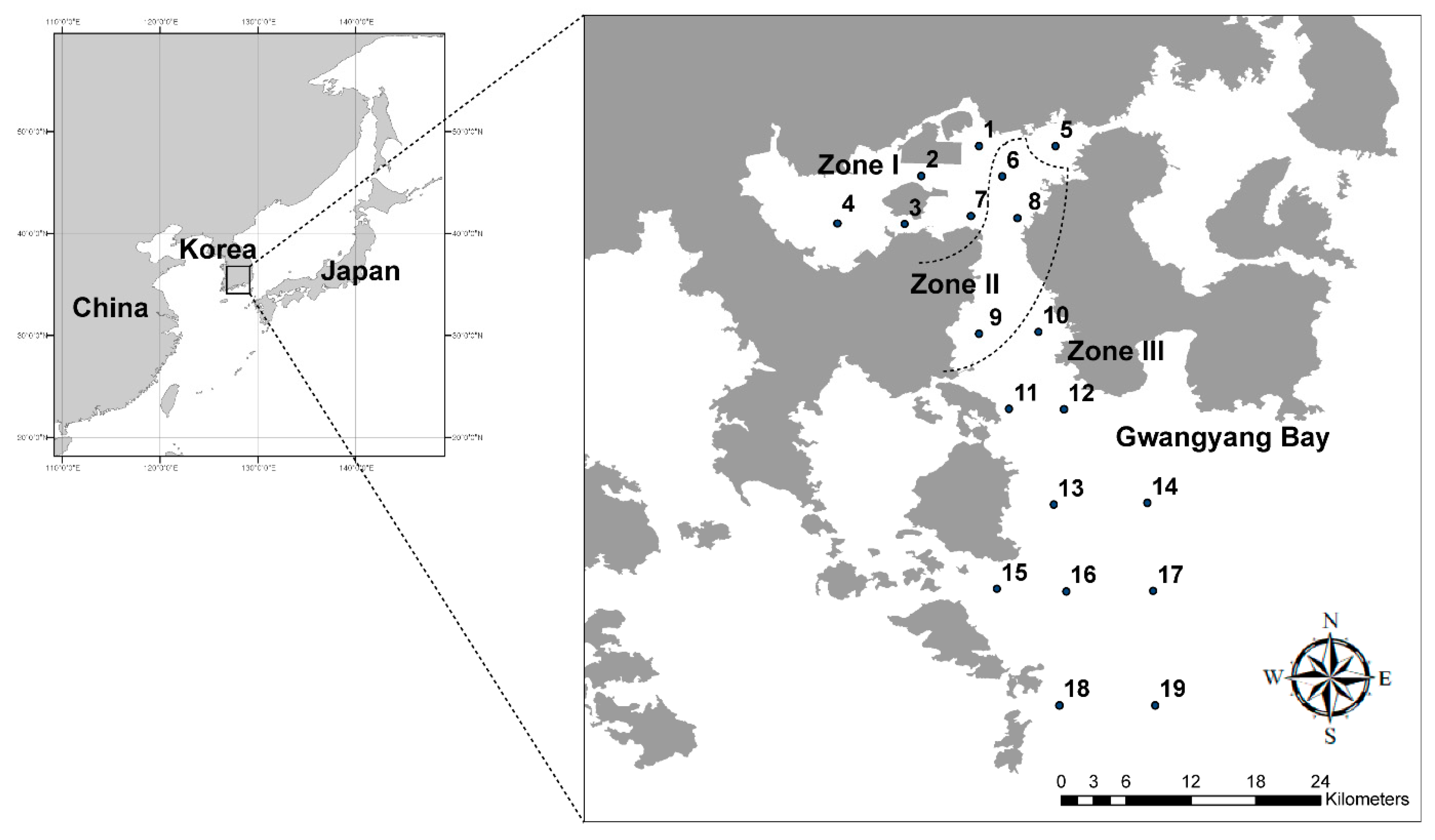
2.1. Study Area

Gwangyang Bay is part of the Korean National Archipelagos located off the south coast of the Korean peninsula (Figure 1). The bay receives an annual mean discharge of 2298 × 106 m3 yr−1 from the Seomjin River [26]. A significant amount of nutrients drains into the system from the watershed (~5000 km2). The water depth varies from 10 m at the Seomjin River estuary to 50 m at the outer Gwangyang Bay. The tidal cycle appears to be semi-diurnal. Compared to other Korean river estuaries which have barriers, the Seomjin River estuary remains open, and thus the water mass is exchanged between the river and ocean more actively. The natural condition of Gwangyang Bay is apt to increase primary productivity as well as biological diversity. In this respect, Gwangyang Bay (~450 km2 from the estuary to the outer bay) is the most economically productive coastal ecosystem in the Korean peninsula [25].

2.2. Sampling, Data Collection and Primer Selection

A survey permitted by Ha-dong local government (permission number: 2010-0165) was conducted in June 2018. We sampled the surface water (approximately the top 50 cm) in this study. In total, nineteen sampling sites were selected, which covered an extensive area from the Seomjin River estuary to the outer Gwangyang Bay (Figure 1). According to Kim et al. [25], at Gwangyang Bay, higher water temperatures corresponded to lower salinity, and vice versa. Phosphorus and nitrogen concentrations were spatially similar across the Bay. Based on the divisions indicated in Kim et al. [25], Zone I covered the inner Bay (sites 3–7, and 9), Zone II represented the main channel of the Bay (sites 8, 10, and 11), and Zone III mostly belonged to the outer Bay (sites 12–21) (Figure 1). Water samples for meta-barcoding analysis (more than 1 L per sample) were obtained at the same time and moved with dry ice to laboratory to filter (0.45 μm pore-size membrane; Advantec MFS membrane filter, Dublin, USA) and stored at −80 °C before NGS analysis. Negative controls were included for every study site to prevent cross contamination. Water temperature and salinity were measured on-site using portable equipment (Model: YSI Professional Plus, OH, USA), while the nutrient and chlorophyll-a concentrations were analyzed in the lab. Phosphorus and nitrogen concentrations were measured using an UV spectrophotometer based on standard analytical methods proposed by the Korean Ministry of Oceans and Fisheries. Chlorophyll-a measurements were also based on UV spectrophotometry. In contrast to nutrient measurements, chlorophyll-a samples were filtered through a 0.45 μm pore-size membrane (Model: Advantec MFS membrane filter). The filter membrane was then homogenized after acetone extraction prior to spectrophotometry. Organic and inorganic carbon concentrations were measured using a carbon analyzer (Model: vario TOC cub, Langenselbold, Germany) using 850 °C combustion catalytic oxidation methods.
We selected the V9 region of the 18S rDNA gene (18S V9), primarily because of its broad range among eukaryotes [27,28]. NGS approaches using the 18S V9 region have recently allowed the characterization of marine planktonic biodiversity in the oceans [29] and prompted biomarker establishment initiatives [30].

2.3. DNA Extraction and Metagenomic Sequencing

Genomic DNA was extracted using PowerSoil® DNA Isolation Kit (Cat. No. 12888, Qiagen, Düsseldorf, Germany) according to the manufacturer’s protocol. DNA extracted for sequencing was prepared according to Illumina 18S Metagenomic Sequencing Library protocols (San Diego, CA, USA). DNA quantity, quality, and integrity were measured by PicoGreen (Thermo Fisher Scientific, Waltham, MA, USA) and VICTOR Nivo Multimode Microplate Reader (PerkinElmer, Akron, OH, USA). The 18S rRNA gene was amplified using 18S V9 primers. The primer sequences are as follows: 18S V9 primer including adaptor sequence (Forward Primer: 5′ TCGTCGGCAGCGTCAGATGTGTATAA GAGACAGCCCTGCCHTTTGTACACAC 3′/Reverse Primer: 5′ GTCTCGTGGGCTCGGAGATG TGTATAAGAGACAGCCTTCYGCAGGTTCACCTAC 3′). To amplify the target region attached with adapters, as a first PCR process, the extracted DNA was amplified by 18S V9 primers with one cycle of 3 min at 95 °C, 25 cycles of 30 s at 95 °C, 30 s at 55 °C, 30 s at 72 °C, and a final step of 5 min at 72 °C for amplicon PCR product. As a second process, to produce indexing PCR, the first PCR product was subsequently amplified with one cycle of 3 min at 95 °C, eight cycles of 30 s at 95 °C, 30 s at 55 °C, 30 s at 72 °C, and a final step of 5 min at 72 °C. The final products were normalized and pooled using PicoGreen (Thermo Fisher Scientific, Waltham, MA, USA), and the size of libraries were verified using the LabChip GX HT DNA High Sensitivity Kit (PerkinElmer, Akron, OH, USA).
The library was sequenced using the MiSeq™ NGS platform (Illumina, San Diego, CA, USA) provided as a commercial service (Macrogen Inc., Seoul, Korea). Raw reads were trimmed with CD-HIT-OTU and chimeras were identified and removed using rDnaTools. For paired-end merging, FLASH (Fast Length Adjustment of SHort reads) version 1.2.11 was used. Merged reads were processed using Qiime version 1.9 [31] and were clustered into operational taxonomic units (OTUs) with UCLUST [32], using a greedy algorithm with OTUs at a 97% OUT cutoff value. Taxonomic classifications were assigned to the obtained representative sequences using BLASTn [33] and UCLUST [32].

2.4. Data Analysis and Statistics

OTUs assigned by meta-barcoding were classified into habitat types (marine, freshwater and estuarine), trophic level (first consumer [filter feeder], second consumer [carnivore], producer and symbiotic) and ISR (indigenous, non-indigenous). Canonical correspondence analysis (CCA) of OTUs exhibiting >1% relative abundance was performed using the PAST 3.0 program [34] to evaluate relationships between abundance of OTU sequences (based on genus level identification) and environmental factors (temperature (Temp.), salinity, total phosphorus (TP), total nitrogen (TN), chlorophyll-a (Chl-a), total organic carbon (TOC), total inorganic carbon (TIC), total carbon (TO), elemental carbon (EC)). All CCA results were constructed using relative abundance data, with natural logarithms transformation (ln 1 + X) used for sample normalization. Linear relationships (Pearson correlations) were calculated between the above environmental factors and classified OTU sequences, based on habitat using XLSTAT version 2018.6.54467 (64 bit) as a plug-in for the Microsoft Excel program [35].

3. Results

3.1. Meta-Barcoding

In total, 3,066,013 paired-end reads from the 19 samples were generated on the Illumina MiSeq™ platform, of which 98.5% passed Q30 (Phred quality score > 30) for improving accuracy of sequences in this study (Supplementary Materials). Each sample yielded paired-end reads ranging from 21,101–299,305 reads (mean: 161,369 reads), which was similar to the amount of reads in the previous study [36], and all samples exhibited saturation of the number of OTUs by rarefaction curve analysis. Gamma-diversity was 352 OTUs produced with a cutoff of 97% similarity. The resulting 352 OTUs were classified into 19 genus-level taxonomic groups (those representing <0.04% abundance were not plotted). Uncultured and non-assigned reads were discarded.

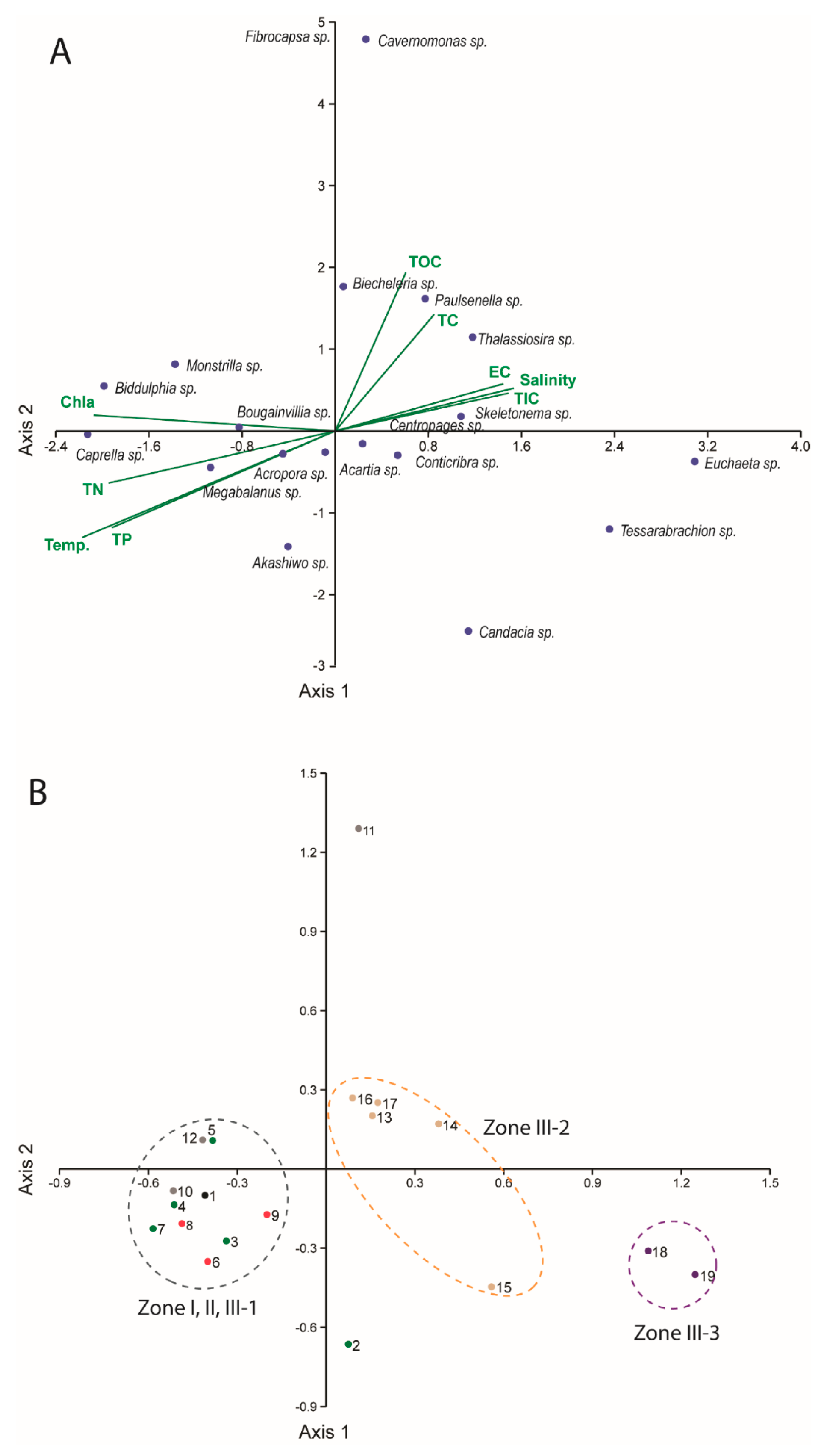
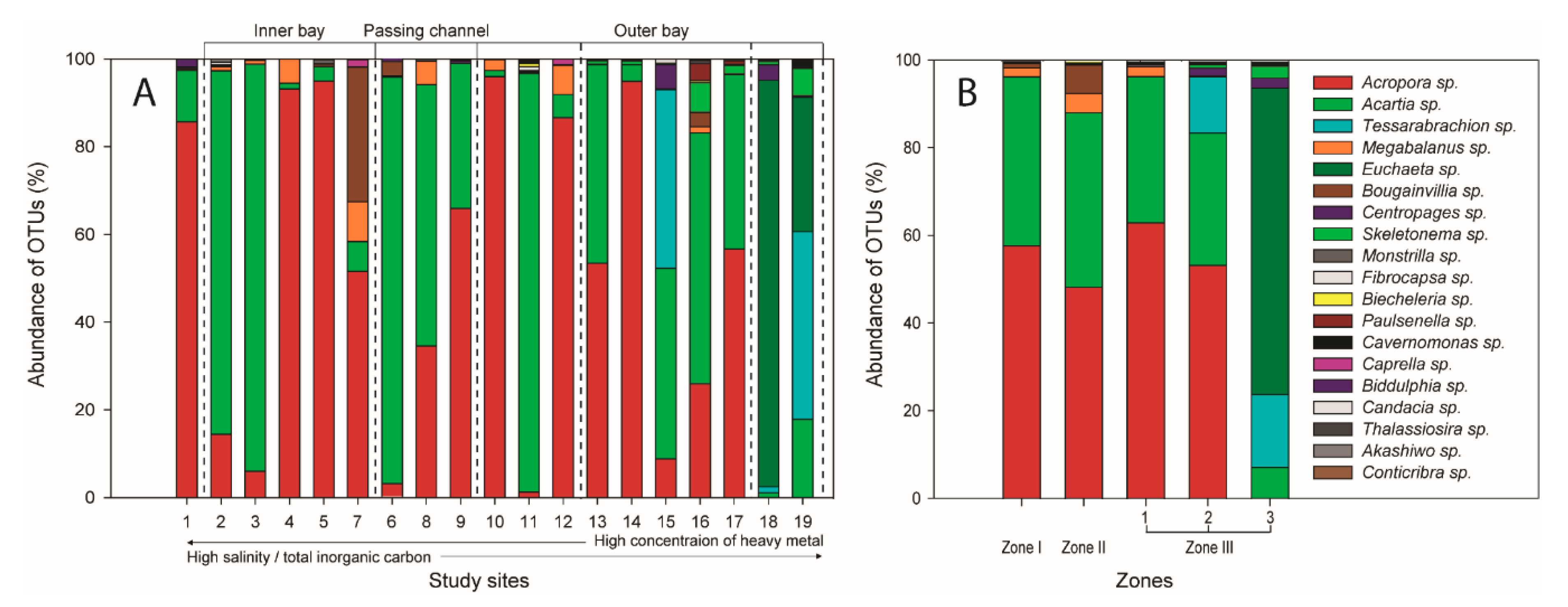
3.2. Spatial Distributions of Aquatic Organisms Based on Meta-Barcoding

We carried out a survey in June 2018. Relationships among the environmental variables and aquatic organisms based on meta-barcoding were explored by CCA (Figure 2). The first axis explained 33.3% of the variance and distinguished Zones III-2 and III-3 with higher salinity, EC, TIC, and lower Chl-a and TN from the other zones. The second axis (19.6% of variance explained) distinguished the sites from Zone III-1 and the other zones, by having higher TOC and TC, lower temperature, and TP. Nutrient-related factors (Chl-a, TN, and TP) were correlated with Acropora sp. (small polyp stony coral) and Megabalanus sp., (barnacle) and salinity was correlated with Skeletonema sp. (diatoms) and Centropages sp. (copepods).
Abundance of assigned OTU sequences showed different patterns among the study sites (Figure 3). The dominant OTU was assigned to Acropora sp. and the sub-dominant OTU was Acartia sp. (copepods). Most common OTUs within the study sites were comprised of phytoplankton, followed by zooplankton and amphipods (Figure 3B). Interestingly, the abundance of OTUs showed different compositions among the three different zones (I, II, III). Zone I showed similar patterns to Zones II and III-1, whereas Zones III-2 and 3 showed different compositions of aquatic organisms which distinguished them from other zones. In particular, Zone III-3 exhibited an entirely different pattern, comprised of marine organisms such as Euchaeta sp. (copepods) and Tessarabrachion sp. (krill) compared with other zone divisions (Figure 3B).

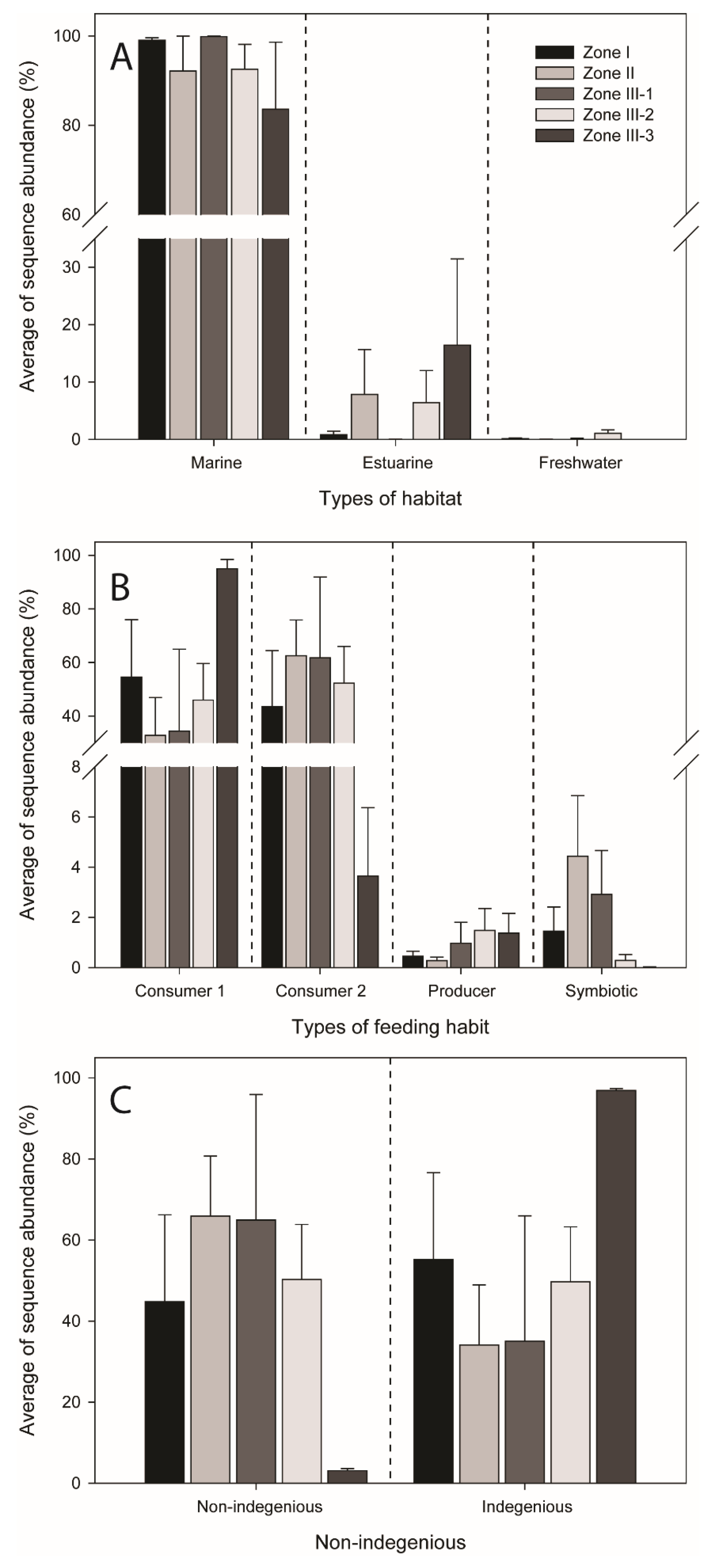
3.3. Functional Features and Non-Indigenous Species

When divided into categories (habitat types, trophic level, and ISR), averages of abundant sequences showed different patterns among the zones (I, II, III-1-2-3). The most dominant habitat type of OTU was the marine type for the three different zones (Figure 4A), while the types of feeding habit and indigenous rate showed complex response patterns. The dominant trophic level was first consumer and second consumer, followed by producer and symbiotic trophic levels (Figure 4B). The indigenous rate of Zone III-3 was significantly higher than other zones, but Zones II and III-1 showed opposite patterns (Figure 4C), while Zones I and III-2 presented no significant difference in indigenous rates. The three divisions of Zone III from CCA results demonstrated similar patterns within the three zone types (Zones I, II-and III).
We found significant relationships between environmental factors (Table 1). Specifically, temperature had positive relationships with nutrient-related factors such as TP and PN, and showed a negative relationship with TOC. Salinity showed significant negative relationships with TN and TP, but also displayed a positive relationship with carbon-related factors such as EC and TC. However, there were no significant relationships between environmental factors and divisions of categories except for habitat types (marine, estuarine, freshwater). The marine habitat of OTUs revealed a significant positive relationship with salinity (r = 0.879) and EC (r = 0.878), respectively, whereas freshwater and estuarine types of OTUs showed negative relationships with salinity (r = −0.888 and −0.856) and EC (r = −0.884 and −0.856) respectively.

4. Discussion

4.1. Effectiveness of eDNA Monitoring

Our results showed that eDNA monitoring based on NGS holds great potential as a complementary monitoring tool to identify spatial taxonomic distribution patterns in coastal areas. We characterized detailed zonation patterns of the outer bay of Gwangyang Bay previously categorized by Kim et al. [25]. Specifically, Zones III-2 and III-3 were clearly resolved by CCA using genus-level identification of aquatic organisms based on meta-barcoding data (Figure 2). When divided into categories (habitat types, trophic level, and ISR), averages of abundant sequences showed different patterns among the zones (I, II, III-1-2-3). The NIS detection of Zone III-3 was significantly higher than the other zones. Therefore, eDNA based on meta-barcoding is a promising ecological tool for monitoring, such as biodiversity assessment or NIS management [24,37,38,39,40].
This approach by meta-barcoding in complex coastal ecosystems confers three distinct advantages over other methods. First, the range of aquatic organisms in coastal ecosystems open to study is widened. Second, identification of aquatic organism to the species or genus level (Appendix A), which can be converted into ecological values such as FFC and NIS, is possible. Finally, sensitivity of the meta-barcoding approach using small volumes of water (1 L) is a promising alternative to traditional methods (i.e., dredges and surber samplers) for biodiversity detection in coastal areas. Using these advantages, eDNA monitoring can provide a useful tool for use in environmental management.
However, some taxa were unable to be identified to the species or genus level due to the incompleteness of reference databases (i.e., NCBI GenBank). More accurate target regions such as the cytochrome oxidase I region, which is called the standard region of barcoding, are needed to identify target species at the species level and are required for identification of aquatic organisms [41]. Another challenge associated with eDNA monitoring is the risk of false-positive and false-negative detections [42]. The reliability of the eDNA sampling method should be demonstrated using in silico, in vitro and in situ validation tests in the coastal area. Even though this approach has limitations, taxonomic expertise is not required and it can supplement observational records and field surveys to obtain marine ecosystem samples and information, as NGS reveals biodiversity and the number of NIS in one specific area along the their temporal and spatial distribution.

4.2. Ecological Values of eDNA Monitoring

Our results showed that Acropora sp. was dominant in terms of abundance of OTU sequences across all study sites, even though it is not a planktonic species. The Acropora colonies post-recruitment by larval recruitment demonstrates higher efficiency for survival than coral-colony growth [43]. It was concluded that larval recruitment largely determines species composition, and that reduced larval recruitment is responsible for the sparse distribution of fragmenting species [44]. Therefore, the larval stage could be easily detected among the study sites by our eDNA monitoring approach. We also found that nutrient-related factors (Chl-a, TN, and TP) were significantly correlated with Acropora sp. and Megabalanus sp. (Figure 2). It is therefore possible that the strong positive correlation between the two species could be the result of coral-inhabiting barnacles [45].
The comprehensive understanding of feeding characteristics of aquatic organisms has not been well elucidated in comparison to their importance [46,47,48,49]. Our results showed that composition of aquatic organisms have different patterns of feeding habits among the three different zone divisions designated by Kim et al. [25] (Figure 4), and we also found similar patterns using CCA based on genus-level identification resulting from our division of Zone III (Figure 2). However, previous research findings were attributed to the absence of adequate information for analysis obtained from the field sites due to difficulties in culture, handling, and identification of eDNA samples derived from bulk sediment and filtered water. In this sense, our results overcame the aforementioned limitations by using a broader detection range for aquatic organisms.
Although, Zhan et al. [50] has described the increased sensitivity of meta-barcoding for NIS, its application for monitoring biological invasion has only recently been demonstrated [51]. In the present work, we identified the utility of meta-barcoding for detection of NIS and their spatial distribution patterns (Figure 4). The reason behind this is the capacity to detect the presence of individuals at early life stages, such as eggs or nauplius larvae, whose identification is difficult with traditional methods [52]. The sensitivity of meta-barcoding, combined with the relatively low time and cost associated with this technique [53], makes it a promising alternative approach for the rapid and accurate detection of biodiversity shifts in aquatic organisms, allowing its potential implementation in environmental policies.

Supplementary Materials

Author Contributions

Conceptualization, H.J., D.-K.K. and I.-S.K.; methodology, H.J. and K.P.; formal analysis, H.J. and D.-K.K.; investigation, H.J. and D.-K.K.; writing—original draft preparation, H.J. and I.-S.K.; writing—review and editing, D.-K.K. and I.-S.K.; project administration, I.-S.K.; funding acquisition, I.-S.K.

Funding

This research was funded by the National Research Foundation of Korea, grant number NRF-2018R1A6A1A03024314.

Conflicts of Interest

The authors declare no conflict of interest.

Appendix A. Species Level Identification List Used in this Paper.

KingdomSpecies
EukaryotaAcropora granulosa
EukaryotaAcartia omorii
EukaryotaTessarabrachion oculatum
EukaryotaMegabalanus stultus
EukaryotaEuchaeta indica
EukaryotaBougainvillia muscus
EukaryotaCentropages typicus
EukaryotaSkeletonema costatum
EukaryotaMonstrilla sp.
EukaryotaFibrocapsa japonica
EukaryotaBiecheleria brevisulcata
EukaryotaPaulsenella vonstoschii
EukaryotaCavernomonas mira
EukaryotaCaprella californica
EukaryotaBiddulphia sp.
EukaryotaCandacia bispinosa
EukaryotaThalassiosira mala
EukaryotaAkashiwo sanguinea
EukaryotaConticribra weissflogiopsis

References

  1. Jo, H.; Ventura, M.; Vidal, N.; Gim, J.S.; Buchaca, T.; Barmuta, L.A.; Erik, J.; Joo, G.J. Discovering hidden biodiversity: The use of complementary monitoring of fish diet based on DNA barcoding in freshwater ecosystems. Ecol. Evol. 2016, 6, 219–232. [Google Scholar] [CrossRef] [PubMed]
  2. Robertson, G.P.; Collins, S.L.; Foster, D.R.; Brokaw, N.; Ducklow, H.W.; Gragson, T.L.; Gries, C.; Hamilton, S.K.; McGuire, A.D.; Moore, J.C.; et al. Long-term ecological research in a human-dominated world. BioScience 2006, 62, 342–353. [Google Scholar] [CrossRef]
  3. Baird, D.J.; Hajibabaei, M. Biomonitoring 2.0: A new paradigm in ecosystem assessment made possible by next-generation DNA sequencing. Mol. Ecol. 2012, 21, 2039–2044. [Google Scholar] [CrossRef] [PubMed]
  4. Myers, R.A.; Worm, B. Rapid worldwide depletion of predatory fish communities. Nature 2003, 423, 280. [Google Scholar] [CrossRef] [PubMed]
  5. Pusceddu, A.; Bianchelli, S.; Martín, J.; Puig, P.; Palanques, A.; Masqué, P.; Danovaro, R. Chronic and intensive bottom trawling impairs deep-sea biodiversity and ecosystem functioning. Proc. Natl. Acad. Sci. USA 2014, 111, 8861–8866. [Google Scholar] [CrossRef] [PubMed] [Green Version]
  6. Ruiz, G.M.; Fofonoff, P.W.; Carlton, J.T.; Wonham, M.J.; Hines, A.H. Invasion of coastal marine communities in North America: Apparent patterns, processes, and biases. Annu. Rev. Ecol. Syst. 2000, 31, 481–531. [Google Scholar] [CrossRef]
  7. Naylor, R.; Williams, S.L.; Strong, D.R. Aquaculture—A gateway for exotic species. Science 2001, 294, 1655–1656. [Google Scholar] [CrossRef]
  8. Padilla, D.K.; Williams, S.L. Beyond ballast water: Aquarium and ornamental trades as sources of invasive species in aquatic ecosystems. Front. Ecol. Environ. 2004, 2, 131–138. [Google Scholar] [CrossRef]
  9. Chapman, J.W.; Miller, T.W.; Coan, E.V. Live seafood species as recipes for invasion. Conserv. Biol. 2003, 17, 1386–1395. [Google Scholar] [CrossRef]
  10. Weigel, S.; Bester, K.; Hühnerfuss, H. Identification and quantification of pesticides, industrial chemicals, and organobromine compounds of medium to high polarity in the North Sea. Mar. Pollut. Bull. 2005, 50, 252–263. [Google Scholar] [CrossRef]
  11. Ardura, A.; Planes, S. Rapid assessment of non-indigenous species in the era of the eDNA barcoding: A Mediterranean case study. Estuar. Coast. Shelf Sci. 2017, 188, 81–87. [Google Scholar] [CrossRef]
  12. Carlton, J.T.; Geller, J.B. Ecological roulette: The global transport of nonindigenous marine organisms. Science 1993, 261, 78–82. [Google Scholar] [CrossRef]
  13. Williams, S.L.; Grosholz, E.D. The invasive species challenge in estuarine and coastal environments: Marrying management and science. Estuaries Coasts 2008, 31, 3–20. [Google Scholar] [CrossRef]
  14. Ogram, A.; Sayler, G.S.; Barkay, T. The extraction and purification of microbial DNA from sediments. J. Microbiol. Meth. 1987, 7, 57–66. [Google Scholar] [CrossRef]
  15. Taberlet, P.; Coissac, E.; Hajibabaei, M.; Rieseberg, L.H. Environmental DNA. Mol. Ecol. 2012, 21, 1789–1793. [Google Scholar] [CrossRef]
  16. Andersen, K.; Bird, K.L.; Rasmussen, M.; Haile, J.; Breuning-Medsen, H.; Kjaer, K.H.; Orlando, L.; Geilbert, M.T.P.; Willerslev, E. Meta-barcoding of ‘dirt’ DNA from soil reflects vertebrate biodiversity. Mol. Ecol. 2011, 21, 1966–1979. [Google Scholar] [CrossRef]
  17. Minamoto, T.; Yamanaka, H.; Takahara, T.; Honjo, M.N.; Kawabata, Z. Surveillance of fish species composition using environmental DNA. Limnology 2012, 13, 193–197. [Google Scholar] [CrossRef]
  18. Thomsen, P.; Kielgast, J.; Iversen, L.L.; Wiuf, C.; Rasmussen, M.; Gilbert, M.T.P.; Orlando, L.; Willerslev, E. Monitoring endangered freshwater biodiversity using environmental DNA. Mol. Ecol. 2012, 21, 2565–2573. [Google Scholar] [CrossRef]
  19. Thomsen, P.; Kielgast, J.; Iversen, L.L.; Møller, P.R.; Rasmussen, M.; Willerslev, E. Detection of a diverse marine fish fauna using environmental DNA from seawater samples. PLoS ONE 2012, 7, e41732. [Google Scholar] [CrossRef]
  20. Yamamoto, S.; Masuda, R.; Sato, Y.; Sado, T.; Araki, H.; Kondoh, M.; Toshifumi, M.; Miya, M. Environmental DNA metabarcoding reveals local fish communities in a species-rich coastal sea. Sci. Rep. 2017, 7, 40368. [Google Scholar] [CrossRef] [Green Version]
  21. Ficetola, G.F.; Miaud, C.; Pompanon, F.; Taberlet, P. Species detection using environmental DNA from water samples. Biol. Lett. 2008, 4, 423–425. [Google Scholar] [CrossRef] [Green Version]
  22. Goldberg, C.S.; Pilliod, D.S.; Arkle, R.S.; Waits, L.P. Molecular detection of vertebrates in stream water: A demonstration using Rocky Mountain tailed frogs and Idaho giant salamanders. PLoS ONE 2011, 6, e22746. [Google Scholar] [CrossRef]
  23. Hawkins, C.P.; Norris, R.H.; Hogue, J.N.; Feminella, J.W. Development and evaluation of predictive models for measuring the biological integrity of streams. Ecol. Appl. 2000, 10, 1456–1477. [Google Scholar] [CrossRef]
  24. Korean Statistical Information Service (KOSIS). Available online: http://kosis.kr (accessed on 9 June 2019).
  25. Kim, D.K.; Jo, H.; Han, I.; Kwak, I.S. Explicit Characterization of Spatial Heterogeneity Based on Water Quality, Sediment Contamination, and Ichthyofauna in a Riverine-to-Coastal Zone. Int. J. Environ. Res. Health 2019, 16, 409. [Google Scholar] [CrossRef]
  26. Kang, C.K.; Kim, J.B.; Lee, K.S.; Kim, J.B.; Lee, P.Y.; Hong, J.S. Trophic importance of benthic microalgae to macrozoobenthos in coastal bay systems in Korea: Dual stable C and N isotope analyses. Mar. Ecol. Prog. Ser. 2003, 259, 79–92. [Google Scholar] [CrossRef]
  27. Abad, D.; Albaina, A.; Aguirre, M.; Laza-Martínez, A.; Uriarte, I.; Iriarte, A.; Arantza, I.; Fernando, V.; Estonba, A. Is metabarcoding suitable for estuarine plankton monitoring? A comparative study with microscopy. Mar. Biol. 2016, 163, 149. [Google Scholar] [CrossRef]
  28. de Vargas, C.; Audic, S.; Henry, N.; Decelle, J.; Mahé, F.; Logares, R.; Lara, E.; Berney, C. Eukaryotic plankton diversity in the sunlit ocean. Science 2015, 348, 1261605. [Google Scholar] [CrossRef] [Green Version]
  29. Albaina, A.; Aguirre, M.; Abad, D.; Santos, M.; Estonba, A. 18S rRNA V9 metabarcoding for diet characterization: A critical evaluation with two sympatric zooplanktivorous fish species. Ecol. Evol. 2016, 6, 1809–1824. [Google Scholar] [CrossRef]
  30. Massana, R.; Gober, A.; Audic, S.; Bass, D.; Bittner, L.; Boutte, C.; Chambouvet, A.; Christen, R. Marine protist diversity in European coastal waters and sediments as revealed by high-throughput sequencing. Environ. Microbiol. 2015, 17, 4035–4049. [Google Scholar] [CrossRef] [Green Version]
  31. Caporaso, J.G.; Kuczynski, J.; Stombaugh, J.; Bittinger, K.; Bushman, F.D.; Costello, E.K.; Huttley, G.A. QIIME allows analysis of high-throughput community sequencing data. Nat. Methods 2010, 7, 335. [Google Scholar] [CrossRef]
  32. Edgar, R.C. Search and clustering orders of magnitude faster than BLAST. Bioinformatics 2010, 26, 2460–2461. [Google Scholar] [CrossRef] [Green Version]
  33. Altschul, S.F.; Gish, W.; Miller, W.; Myers, E.W.; Lipman, D.J. Basic local alignment search tool. J. Mol. Biol. 1990, 215, 403–410. [Google Scholar] [CrossRef]
  34. Hammer, Ø.; Harper, D.A.; Ryan, P.D. PAST: Paleontological statistics software package for education and data analysis. Palaeontol. Electron. 2001, 4, 9. [Google Scholar]
  35. Addinsoft. XLSTAT Statistical and Data Analysis Solution; Addinsoft: New York, NY, USA, 2019. [Google Scholar]
  36. Thomsen, P.F.; Møller, P.R.; Sigsgaard, E.E.; Knudsen, S.W.; Jørgensen, O.A.; Willerslev, E. Environmental DNA from seawater samples correlate with trawl catches of subarctic, deepwater fishes. PLoS ONE 2016, 11, e0165252. [Google Scholar] [CrossRef]
  37. Bourlat, S.J.; Borja, A.; Gilbert, J.; Taylor, M.I.; Davies, N.; Weisberg, S.B.; Glöckner, F.O. Genomics in marine monitoring: New opportunities for assessing marine health status. Mar. Pollut. Bull. 2013, 74, 19–31. [Google Scholar] [CrossRef]
  38. Valentini, A.; Taberlet, P.; Miaud, C.; Civade, R.; Herder, J.; Thomsen, P.F.; Bellemain, E.; Besnard, A.; Coissac, E.; Boyer, F.; et al. Next-generation monitoring of aquatic biodiversity using environmental DNA barcoding. Mol. Ecol. 2016, 25, 929–942. [Google Scholar] [CrossRef] [PubMed]
  39. O’Donnell, J.L.; Kelly, R.P.; Shelton, A.O.; Samhouri, J.F.; Lowell, N.C.; Williams, G.D. Spatial distribution of environmental DNA in a nearshore marine habitat. Peer J. 2017, 5, e3044. [Google Scholar] [CrossRef] [PubMed]
  40. Djurhuus, A.; Pitz, K.; Sawaya, N.A.; Rojas-Márquez, J.; Michaud, B.; Montes, E.; Muller-Karger, F.; Breitbart, M. Evaluation of marine zooplankton community structure through environmental DNA metabarcoding. Limnol. Oceanogr. Methods 2018, 16, 209–221. [Google Scholar] [CrossRef] [Green Version]
  41. Hajibabaei, M.; Smith, M.A.; Janzen, D.H.; Rodriguez, J.J.; Whitfield, J.B.; Hebert, P.D. A minimalist barcode can identify a specimen whose DNA is degraded. Mol. Ecol. Notes 2006, 6, 959–964. [Google Scholar] [CrossRef]
  42. Darling, J.A.; Mahon, A.R. From molecules to management: Adopting DNA-based methods for monitoring biological invasions in aquatic environments. Environ. Res. 2011, 111, 978–988. [Google Scholar] [CrossRef]
  43. Victor, S.; Golbuu, Y.; Yukihira, H.; van Woesik, R. Acropora size-frequency distributions reflect spatially variable conditions on coral reefs of Palau. Bull. Mar. Sci. 2009, 85, 149–157. [Google Scholar]
  44. Wallace, C.C. Reproduction, recruitment and fragmentation in nine sympatric species of the coral genus Acropora. Mar. Biol. 1985, 88, 217–233. [Google Scholar] [CrossRef]
  45. Lewis, J.B. Recruitment, growth and mortality of a coral-inhabiting barnacle Megabalanus stultus (Darwin) upon the hydrocoral Millepora complanata Lamarck. J. Exp. Mar. Biol. Ecol. 1992, 162, 51–64. [Google Scholar] [CrossRef]
  46. Rothhaupt, K. Differences in particle size-dependent feeding efficiencies of closely related rotifer species. Limnol. Oceanogr. 1990, 35, 16–23. [Google Scholar] [CrossRef]
  47. Thouvenot, A.; Debroas, D.; Richardot, M.; Devaux, J. Impact of natural metazooplankton assemblage on planktonic microbial communities in a newly flooded reservoir. J. Plankton Res. 1999, 21, 179–199. [Google Scholar] [CrossRef] [Green Version]
  48. Mohr, S.; Adrian, R. Reproductive success of the rotifer Brachionus calyciflorus feeding on ciliates and flagellates of different trophic modes. Freshwater Biol. 2002, 47, 1832–1839. [Google Scholar] [CrossRef]
  49. Devetter, M.; Sed’a, J. Rotifer fecundity in relation to components of microbial food web in a eutrophic reservoir. Hydrobiologia 2003, 504, 167–175. [Google Scholar] [CrossRef]
  50. Zhan, A.; Hulak, M.; Sylvester, F.; Huang, X.; Adebayo, A.A.; Abbott, C.L.; Adamowicz, S.J.; Heath, D.D. High sensitivity of 454 pyrosequencing for detection of rare species in aquatic communities. Methods Ecol. Evol. 2013, 4, 558–565. [Google Scholar] [CrossRef]
  51. Zaiko, A.; Samuiloviene, A.; Ardura, A.; Garcia-Vazquez, E. Metabarcoding approach for nonindigenous species surveillance in marine coastal waters. Mar. Pollut. Bull. 2015, 100, 53–59. [Google Scholar] [CrossRef]
  52. Comtet, T.; Sandionigi, A.; Viard, F.; Casiraghi, M. DNA (meta) barcoding of biological invasions: A powerful tool to elucidate invasion processes and help managing aliens. Biol. Invasions 2015, 17, 905–922. [Google Scholar] [CrossRef]
  53. Kelly, R.P.; Port, J.A.; Yamahara, K.M.; Martone, R.G.; Lowell, N.; Thomsen, P.F.; Mach, M.E.; Bennett, M. Environmental monitoring. Harnessing DNA to improve environmental management. Science 2014, 344, 1455–1456. [Google Scholar] [CrossRef]
Figure 1. Map of the study sites with division of zones referred to by Kim et al. (2019) [25].
Applsci 09 03450 g001
Figure 2. Canonical correspondence analysis (CCA) used to evaluate (A) the relationships between abundance of operational taxonomic units (OTUs) sequences (based on genus level identification) and environmental factors (temperature (Temp.), Salinity, total phosphorus (TP), total nitrogen (TN), chlorophyll-a (Chl-a), total organic carbon (TOC), total inorganic carbon (TIC), total carbon (TO), elemental carbon (EC)). (B) Sites grouping based on CCA analysis.
Applsci 09 03450 g002
Figure 3. Abundance of OTU sequences along the study sites (A) with site description of physical features and zone classification (B) based on genus identification level.
Applsci 09 03450 g003
Figure 4. Comparison of the habitat types ((A), marine-freshwater-estuarine), trophic level ((B), consumer 1 [filter feeder], consumer 2 [carnivore], producer and symbiotic) and natives ((C), non-indigenous and indigenous) among five zoning types based on genus identification level.
Applsci 09 03450 g004
Table 1. Linear relationship (Pearson correlation) between environmental factors (temperature (Temp.), Salinity, total phosphorus (TP), total nitrogen (TN), chlorophyll-a (Chl-a), total organic carbon (TOC), total inorganic carbon (TIC), total carbon (TO), elemental carbon (EC)) and classified OTU sequences based on habitat types, feeding habits and natives (Bold: significant relationship).
VariablesTempSalinityECTPTNTOCTICTCChla
Temp1−0.192−0.2160.5050.464−0.599−0.275−0.2200.422
Salinity−0.19210.996−0.586−0.5320.3010.4350.4860.006
EC−0.2160.9961−0.615−0.5640.3250.4400.478−0.034
TP0.505−0.586−0.61510.904−0.505−0.634−0.7150.192
TN0.464−0.532−0.5640.9041−0.424−0.680−0.6450.200
TOC−0.5990.3010.325−0.505−0.42410.1270.355−0.248
TIC−0.2750.4350.440−0.634−0.6800.12710.8770.195
TC−0.2200.4860.478−0.715−0.6450.3550.87710.263
Chl−a0.4220.006−0.0340.1920.200−0.2480.1950.2631
Marine−0.1970.8790.878−0.343−0.1950.3140.0510.151−0.082
Fresh0.123−0.888−0.8840.3320.199−0.286−0.061−0.1750.024
Estuarine0.269−0.856−0.8560.3490.188−0.337−0.041−0.1230.139
First consumer0.195−0.283−0.2710.1640.1200.152−0.329−0.2690.159
Second consumer0.0110.3870.373−0.329−0.0700.1590.2390.3460.026
Producer−0.054−0.319−0.3070.2880.040−0.194−0.162−0.281−0.064
Symbiotic0.032−0.335−0.3260.2660.1820.158−0.298−0.3010.220
Non-indigenous−0.002−0.348−0.3310.2840.021−0.137−0.195−0.295−0.008
Indigenous0.0020.3480.331−0.284−0.0210.1370.1950.2950.008

