1. Introduction
The robot can perform many tasks in order to help human beings in industrial fields. For example, machining and welding are classical. It is necessary to study the factors that are the obstacles for the improvement of the robot tasks. The classical applications in a factory usually generate forces and torques at the end-effector (EE) of the industrial robot, and the stiffness is the factor that should be considered in order to obtain good performance. The industrial robot requires suitable compliance while performing industrial tasks. Especially when the industrial robot performs the tasks with a high precision requirement, the accuracy of the EE is often influenced by the stiffness characteristic. Lots of attention has been directed at studying the factors that influence the accuracy of the EE and how to deal with these issues [
1,
2]. One solution to this problem is to identify the stiffness parameters of the industrial robot and then use the deformation compensation algorithm to improve the performance of the robot’s tasks. The joint stiffness identification is one aspect of robot calibration. Some researchers have studied robot calibration and defined three levels of calibration methods. Roth presented the analysis of calibration methods for the robot, and stiffness identification belongs to the level of non-geometric calibration [
3]. Many researchers have studied how to improve the accuracy of the EE and the performance of the robot force control while considering stiffness. These efforts led to joint stiffness modeling and stiffness identification of the robot, and there are some groups of stiffness identification algorithms. For example, the finite elements analysis (FEA) method constructs the physical model based on many of finite elements and the corresponding relative stiffness matrices [
4,
5,
6]. Mekaouche presented a method of evaluating the relationship between a numerical tool and a general stiffness map of the robot based on FEA [
7]. The matrix structure analysis (MSA) method uses beams and nodes to construct the stiffness model under the assumption that the links are not subject to bending [
8]. Deblaise [
8] proposed a method to calculate the parallel kinematic machines based on matrix structural analysis in a closed form, and the method can obtain high accuracy specifications. The virtual joint method (VJM) uses the idea of rigid links and compliant joints, and then the calculation of the Jacobian matrix is needed to formulate the stiffness model [
9]. Klimchik presented an approach to identify the elastostatic parameters of both links and joints in a real industrial environment based on VJM, and this approach comprises of physical algebraic and statistical model reduction methods [
10]. The compliance is important for the analysis of mechanism stiffness characteristics in Cartesian space [
11,
12,
13,
14,
15]. The stiffness characteristics of industrial robots influence the requirement of the accuracy and the force commands [
16]. Numerous papers concern the stiffness analysis and optimization in order to improve the accuracy of the location of the EE as well as the force control [
17,
18]. Therefore, in order to obtain a broad, successful application, the industrial robot must have reasonable elastostatic performance. Shin et al. studied the stiffness model of redundant parallel kinematic mechanisms (PKM) and presented a decoupling method for explicit stiffness analysis of redundant PKM. After that, they discussed the optimization and control of the PKM when external forces were applied to the mechanisms [
19]. He et al. studied the stiffness model and the structural parameters of a multibackbone continuum robot based on screw theory, and then obtained the relationship between the force and the deformation of the continuum robot. Then, a theoretical real-time control algorithm was provided based on the stiffness analysis [
20]. Dao studied the compliant guiding mechanism (CGM) in order to improve the performance of the micro/nanoindentation devices and using a hybrid approach of Taguchi-grey based on fuzzy logic to select the appropriate parameters for good compliance of the mechanism [
21]. Luo et al. studied the structure mechanism of the slender robot arm and proposed a structural optimization method to optimize the sensitive design variables of the slender robot arm. The stiffness of the robot arm was enhanced by the proposed optimization method regardless of constant forces or variable forces [
22]. Chen presented the theory of mapping the relationship between joint and Cartesian space, then the author proposed the conservative congruence transformation (CCT) theory in order to identify the stiffness parameters properly [
23].
The robotics community has paid lots of attention to the utilization of dual quaternion algebra, as the representation of position and orientation based on dual quaternions is efficient and singularity-free [
24,
25,
26]. Clifford is the first one who combined the dual number with the quaternion and got the dual number quaternion, which can be used for the analysis of a rigid body in space [
27]. The dual number quaternion, which is also called dual quaternions, is used as the transformation operator and it can represent the rotation and translation of a rigid body in space simultaneously. The advantage of representation based on dual quaternion algebra is that the dual quaternion offers a computationally efficient way to establish the model of the robot in kinematic analysis [
28,
29,
30]. The dual quaternion was used to formulate the calibration algorithms by many researchers. For example, Daniilidis [
31] proposed an algorithm for hand-eye calibration based on dual quaternions. This method can solve hand-eye rotation and translation problems simultaneously. It is necessary to pay attention to optimizing stiffness properties of the robot, as the stiffness analysis is an effective way to improve the performance of the robot operation. The dual quaternion can also be used to formulate the control algorithm and is useful for robot stiffness analysis. Otherwise, it is convenient to compensate the pose error of the EE by the deformation compensation algorithm based on dual quaternion algebra during the robot task. As the industrial robot has become more and more popular in the modern world, so it is necessary to improve the stiffness performance during the application.
This paper focuses primarily on joint stiffness identification and deformation compensation of serial industrial robots. The paper is structured as follows.
Section 2 briefly introduces the forward kinematics of industrial robots based on dual quaternion algebra and the corresponding Jacobian matrix. In
Section 3, the joint stiffness model and stiffness identification algorithm of serial robots based on dual quaternion algebra are presented. The deformation compensation algorithm based on dual quaternion algebra is presented in
Section 4.
Section 5 presents the experiment and analysis of the proposed stiffness modeling and deformation compensation algorithm.
Section 6 summarizes the paper.
2. Forward Kinematics and Jacobian Matrix
This section focuses on the geometric background of dual quaternion algebra and some relevant properties. Readers can find more detail on these concepts in the literature [
24,
25,
26,
27,
28,
29,
30,
31]. The dual quaternion algebra offers a concise and efficient mathematical way to represent rotation and translation of the rigid body simultaneously. The motion of the EE of industrial robots can be expressed by dual quaternions as well. Aspragathos [
24] compared dual quaternion algebra with the homogeneous transformation method (HTM) in terms of representation, storage, and computational efficiency. The author found that dual quaternions have an elegant representation and requires less memory locations. Moreover, the dual quaternion needs less addition, subtraction, multiplication, and division operations as the number of degree of freedom (DOF) increases. The formulations of the kinematic model and stiffness modeling are efficient and compact based on dual quaternion algebra.
A dual quaternion is defined as
A dual quaternion can be separated into the real part
and the dual part
In this paper, a convenient notation of a dual quaternion is given below:
The conjugate of a dual quaternion used in this paper is given by
Define “
” as the multiplication operator of two dual quaternions. Then we get
where
and
are the real parts of
and
respectively,
and
are the dual parts of
and
, respectively.
The operator “
” is an arithmetic product of two quaternions, and this product is given below:
where
and
are scalar parts of
and
respectively,
and
are vector parts of
and
, respectively.
Before formulating the kinematic equations of the robot, the robot parameter definition is important for the kinematic model. Even though the established kinematic model based on dual quaternion algebra is different from the Denavit–Hartenberg (DH) model, the DH notation can also be used by the dual quaternion algebra [
24].
Considering the single link’s parameters based on the DH notation, the forward kinematic model of an n-link serial robot with respect to the fixed base coordinate frame can be calculated as
where
.
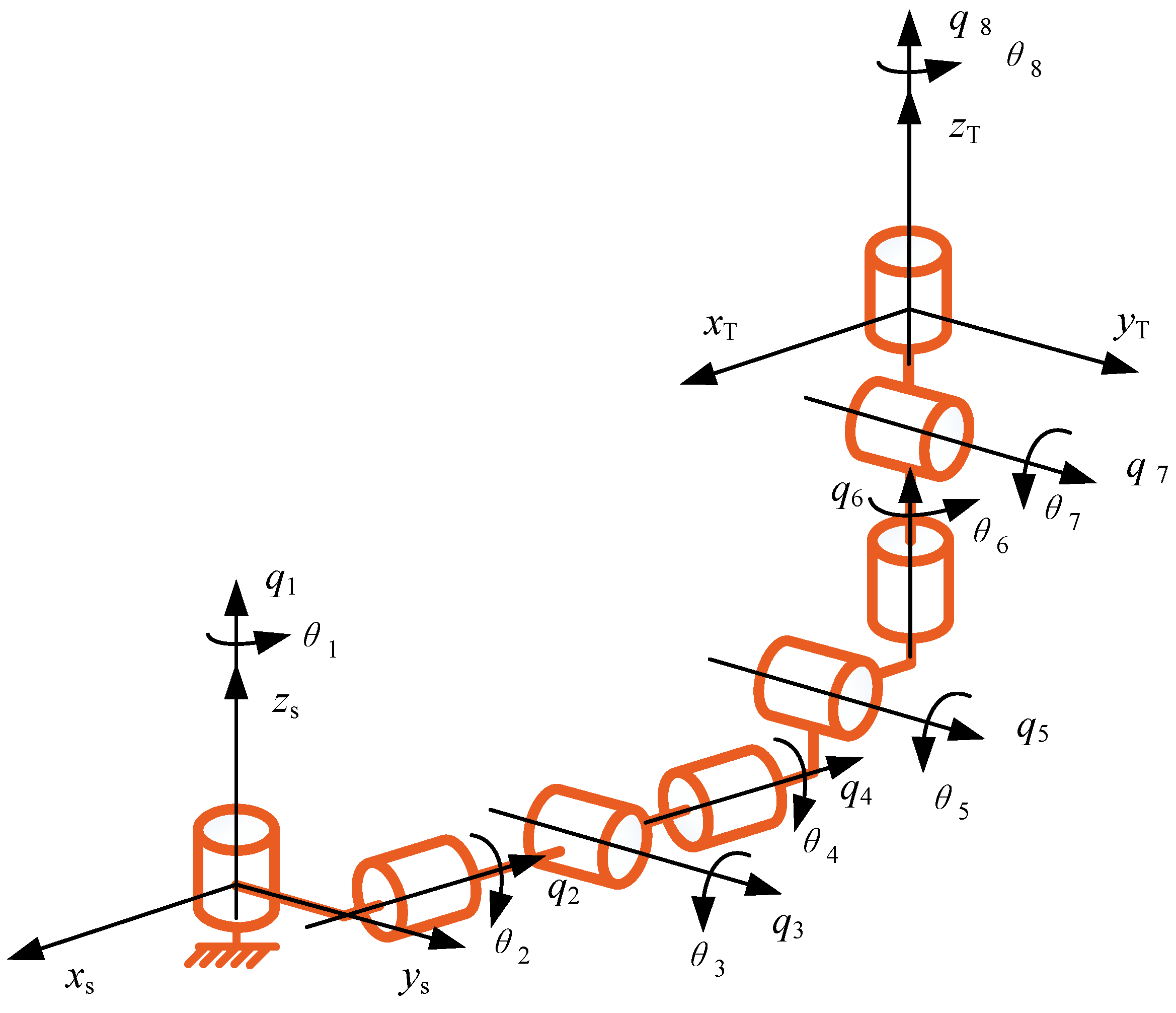
Equation (8) can formulate the forward kinematic equation of an 8-DOF serial industrial robot shown in
Figure 1, which depicts one arm of the dual arm robot used next in the experiment. The relationship between joint velocity and the velocity of the EE in Cartesian space is represented by the Jacobian matrix. This well-known relationship is
where
is the velocity of the EE, and
is the Jacobian matrix.
In the dual quaternion space, the Jacobian matrix just relates the joint velocity vector
and the time derivative of the dual quaternion. The relationship used in this paper is given below:
where
is the dual quaternion calculated by Equation (8), which represents the position and orientation of the EE.
Then, the Jacobian matrix in the dual quaternion space is given by
3. Joint Stiffness Modeling and Identification
The stiffness transformation that relates the joint stiffness of a robot to the stiffness characteristics in a workspace is essential to the improvement of the EE localization, and the stiffness characteristics are important for the force improvement of industrial robots. Thus, the stiffness transformation is critical to the stiffness modeling. The CCT theory is a valid and complete stiffness-mapping algorithm in the stiffness analysis of industrial robots [
23], and dual quaternion algebra can also be used to formulate the compliance model with respect to the CCT theory. Before the formulation of the stiffness modeling below, it is necessary to make three assumptions. First, the EE of the robot is rigid, and the weak stiffness of the robot is the major cause of the deformations. Second, the elastic deformation of the joints causes the displacement, and the links of the robot are rigid. Third, the operation of robot task is under stable conditions. In addition, the external load is the sole factor that influences the deformation.
The external force and torque applied to the EE can cause the EE to experience a small change. The infinitesimal displacement
of the EE of the industrial robot represented by the infinitesimal joint angle
is given by
The principle of virtual work is considered in the formulation, and the dual quaternion form of virtual work of the serial robot that has n revolute joints is given by
where
is the circle product [
29],
is the work represented in joint space,
is the
-th dual force applied to
-th joint of an industrial robot, “
” means the scalar part of the dual quaternion.
In addition, the dual quaternion form of the virtual work of the EE is given by
where
is the work done by the EE,
is the dual force applied to the EE of the industrial robot,
is the dual displacement of the EE.
A dual quaternion has a real part and a dual part. In addition, both of these two parts have a scalar part and a vector part, respectively. Extract the scalar parts from
and
and we have
where
and
are the real part and the dual part of
, respectively,
and
are the real part and the dual part of
, respectively.
The linear algebra can be applied to the calculation of dual quaternion algebra. Thus, Equation (15) can be rewritten in the form of matrices for convenient calculation, and the equation is given by
where
is the modified torque vector,
is the joint angle vector,
is the force and torque applied to the EE,
denotes small displacement,
, and all of these elements are represented in dual quaternion space by matrix form.
The displacement
in Equation (16) can be represented by the Jacobian matrix and the corresponding infinitesimal elements. The relationship is given by
where
is the Jacobian matrix, and
contains the variables of the EE.
Substitute Equation (17) into Equation (16), and the following relationship is obtained
The relationship between the torque
and joint angle
is given by
where
is the diagonal matrix which represents the joint stiffness matrix.
Dual quaternion algebra can also be used to represent
and
. Equation (19) can be expressed as
where
is the torque vector,
and
are dual matrices, respectively.
Combining Equations (18) and (20), we obtain the following relationship based on linear matrix algebra
where
is the joint stiffness matrix represented in dual quaternion space.
The relationship between external force
and the Cartesian infinitesimal displacement
based on dual quaternion algebra is written as
where
is the diagonal Cartesian stiffness matrix, and
is the displacement of the EE.
By using the matrix and Taylor’s expansion, Equation (24) can be rewritten in the following form
where
is the modified joint stiffness matrix, and
is the displacement of the EE; both of them are represented in dual quaternion space.
By differentiating the transpose of Equation (18), the following relationship is obtained
Using Equation (25), Equation (26) can be rearranged as
where
is the modified dual quaternion.
Equation (27) can be rewritten as
where
is the modified Jacobian matrix,
is the complementary stiffness matrix,
is the joint stiffness matrix. The complete stiffness matrix of the industrial robot can be written as
The following relationship is obtained:
where
is the deflection dual quaternion.
Equation (30) can be expressed in the following form
where
Equation (31) can be solved by the least-squares algorithm and the solution is expressed by
Dual quaternion algebra is used to calculate and in the convenient way, and then the stiffness identification result can be obtained by solving Equation (35). After identification, the joint stiffness parameters are used in the next compensation procedure that improves the performance of industrial robots.
5. Experiment and Analysis
In order to verify the effectiveness of the stiffness identification algorithm and the deformation compensation algorithm presented above, a real experiment has been conducted on an industrial robot. The stiffness parameters were identified during the experiment first, and then the estimated parameters were used to calculate the deformation caused by the given load for the simulation. After that, the deformation compensation algorithm was applied to the real drilling operation which was performed by an industrial robot.
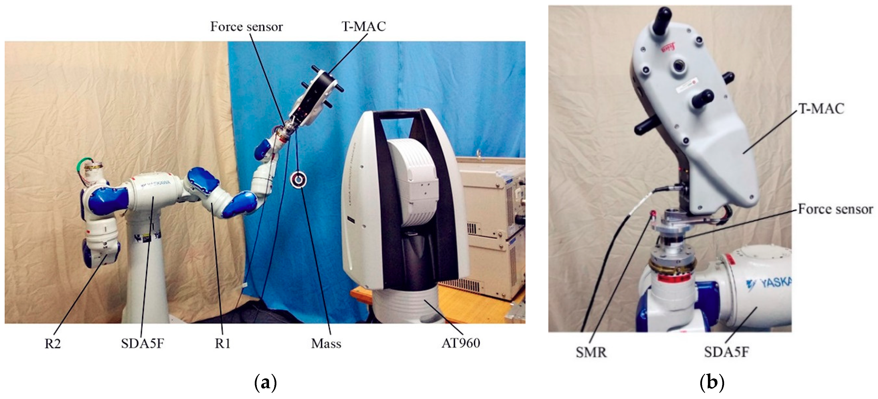
Figure 3 shows the experimental setup. The experiment contained a dual arm industrial robot SDA5F, Leica Geosystems Absolute Tracker (AT960), and tracker machine control probe (T-MAC). T-MAC stands for tracker machine control probe, which was used to measure the pose of the rigid body. The DH parameters of robot SDA5F were used to formulate the forward kinematic model based on dual quaternion algebra, and then the stiffness modeling was established. Each arm of SDA5F was a serial chain manipulator, and these two arms were called R1 and R2, respectively. R1 was the left arm of SDA5F, R2 was the right arm of SDA5F. The R2 had the same joint configuration as R1, and they were symmetric about the base axis. Each arm had 7 revolute joints, and the robot had 15 revolute joints in total. The DH parameters of R1 and R2 are shown in
Table 1 and
Table 2, respectively.
Figure 3a shows that a mass block was applied to the robot EE. The Leica Geosystems Absolute Tracker (AT960) was fixed outside the workspace of SDA5F.
Figure 3b shows the installation of the TMAC. The force sensor was mounted on the EE of the robot. The T-MAC was mounted on the force sensor, and a spherically mounted reflector (SMR) was mounted near the mounting interface of T-MAC. The measurement uncertainty of the measuring machine was
.
From Equation (35), the joint stiffness can be identified by the given forces and torques measured at the EE. Furthermore, by giving joint stiffness parameters, external forces and torques, it is convenient to calculate the deflection or deformation
in return. First, the force sensor measured the forces and torques caused by the mass at the EE when the arm was at different poses. Then, the measurements were taken into the transformation in order to obtain vertical elements that were used to identify the joint stiffness by Equation (35). The procedure usually needs to measure several poses of the EE and then the following equation can be obtained:
where
, and
,
is the number of measurements.
The solution of Equation (46) can be expressed by
After the measurements of the deformation and the forces and torques, Equation (47) is used to calculate the estimated values of the joint stiffness. The results of the identification were the statistical average of several calculation values, and they are listed in
Table 3 and
Table 4. The estimated values are not big, and this is similar to the joint stiffness characteristic of the industrial robot as expected, according to Reference [
9].
These two arms had the same mechanism topology, but the estimated values of the joint stiffness of R1 were not the same as those of R2. This is because the identification results were the theoretical values that can be affected by the measurement noise, calculation errors, postures of the arm, installation environment, and so on.
After the identification, the estimated values of joint stiffness were used to calculate the deformation of the EE under the given external load. The pose error
between the nominal value and the calibrated value is divided into the position error
and the orientation error
in this paper:
where
and
are the estimated position value and orientation values, respectively,
and
are the ideal position value and orientation values, respectively.
The norm value computed by the vector components of position error
is calculated by
where
is the error along the
-axis direction,
is the error along the
-axis direction,
is the error along the
-axis direction. Similarly, the norm value computed by the vector components of orientation error
is calculated by
where
is the error around the
-axis direction,
is the error around the
-axis direction,
is the error around the
-axis direction.
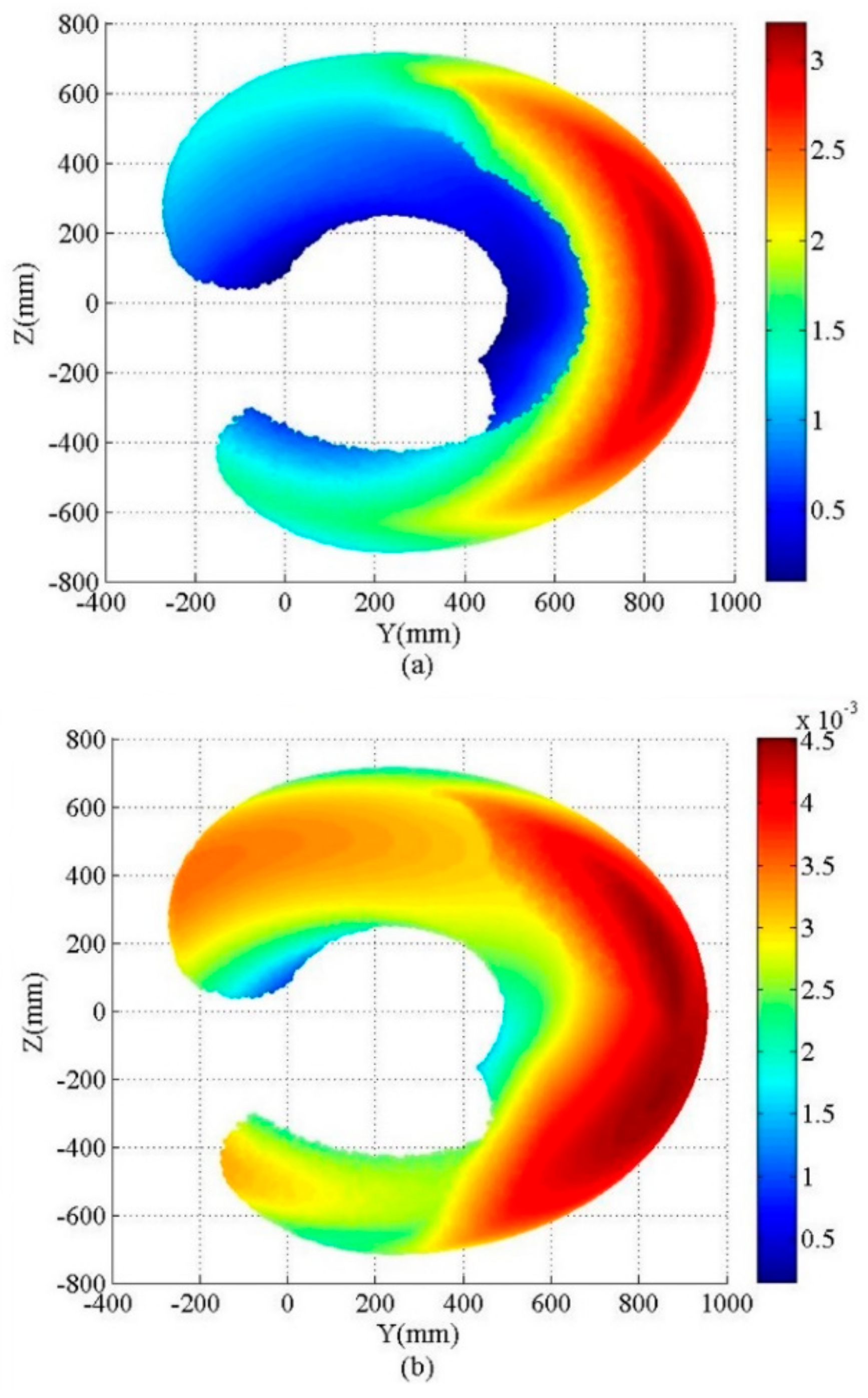
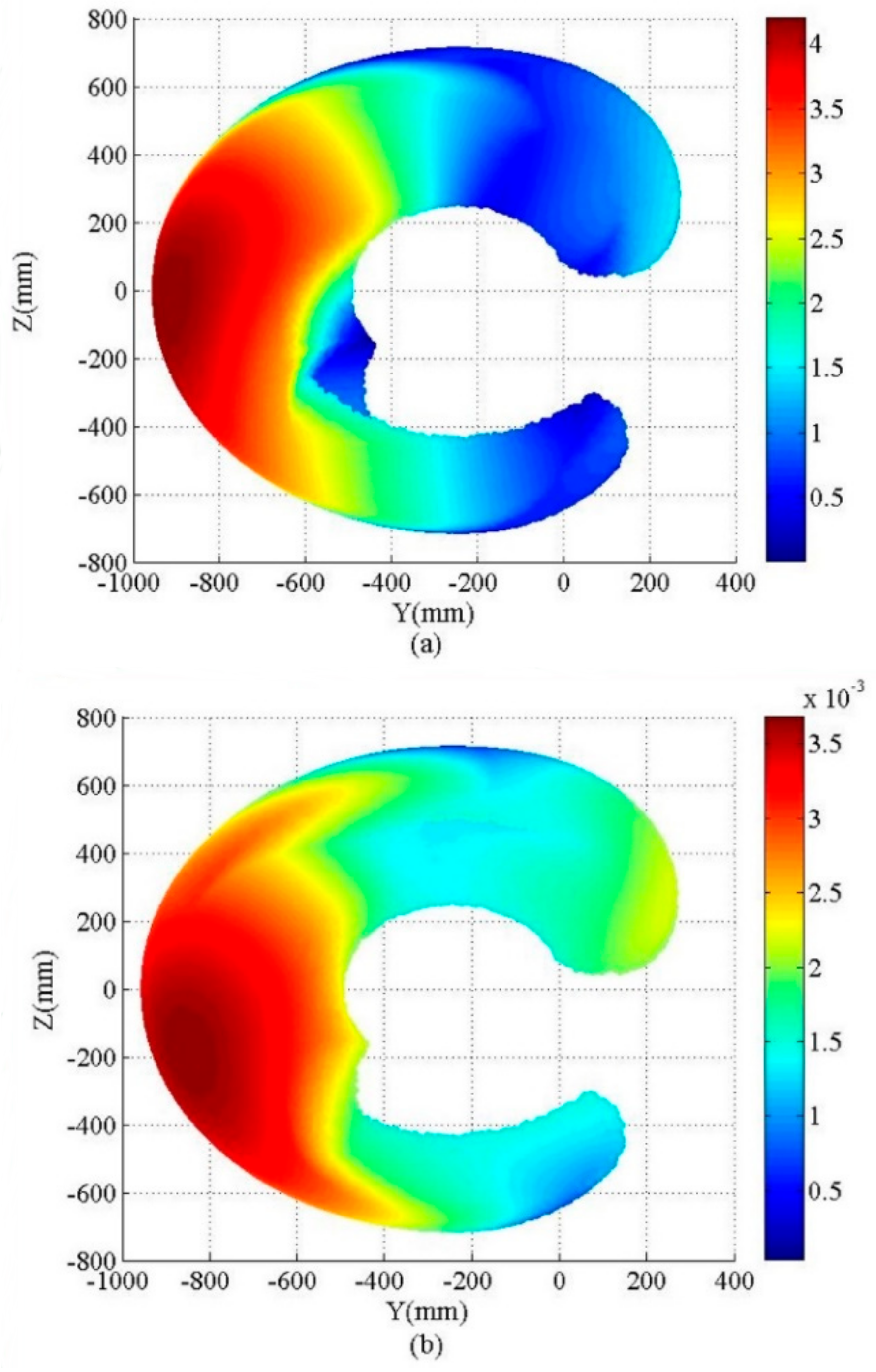
After the joint stiffness identification, a given load was added to the EE and the deformation was calculated for the simulation first. The given load was a dumbbell with a mass of 0.153 kg.
Figure 4 and
Figure 5 depict the error between the nominal pose and the actual pose caused by the deformation throughout the robot workspace. The analysis result shows that the position error of R1 was in the range [0, 3.5] (in millimeters), and the orientation error of R1 was in the range [0, 0.0045] (in radians). The position error of R2 was in the range [0, 4.2] (in millimeters), and the orientation error of R2 was in the range [0, 0.0037] (in radians). The different deformation between the two arms was because of the difference in the mechanism and the measurement results.
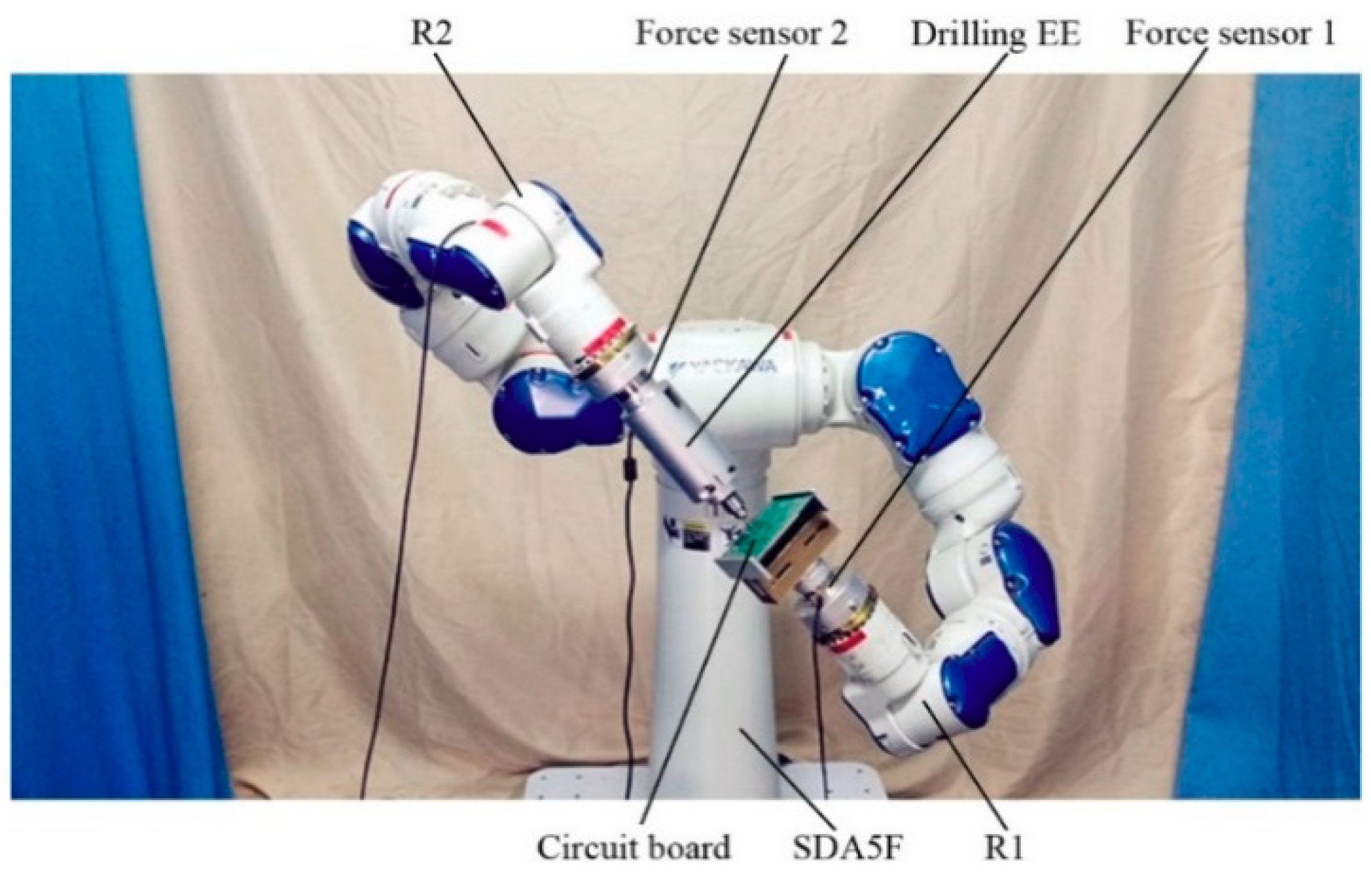
The drilling procedure is typical in manufacturing, and industrial robots can perform the drilling task as they have high flexibility and low cost. The SDA5F is also a humanoid robot, which is useful in mimicking human beings during manufacturing. In the electrical industry, drilling on circuit boards is a common procedure, and manual drilling is labor-intensive and heavy for a human. The drilling procedure is accomplished by automatic mechanisms usually, thus, SDA5F performed the drilling procedure on the circuit board during the experiment.
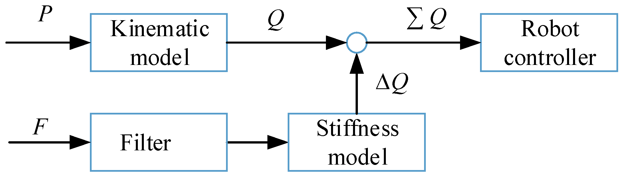
Figure 6 shows the experimental setup. Two six-axis force sensors were mounted on the flanges of R1 and R2, respectively. The circuit board was fixed by the fastening tool, which was mounted on the force sensor 1. The drilling EE was mounted on one side of the force sensor 2. The weights of the drilling EE, fastening tool, and force sensors were measured before their installation. From Equation (44), the deformation can be calculated and compensated to the pose control of the robot. Ten poses were measured with and without the compensation first, and the results were used to calculate the deformation as shown in
Figure 7 and
Figure 8. The error of position and orientation of both arms are calculated by Equations (49) and (50).
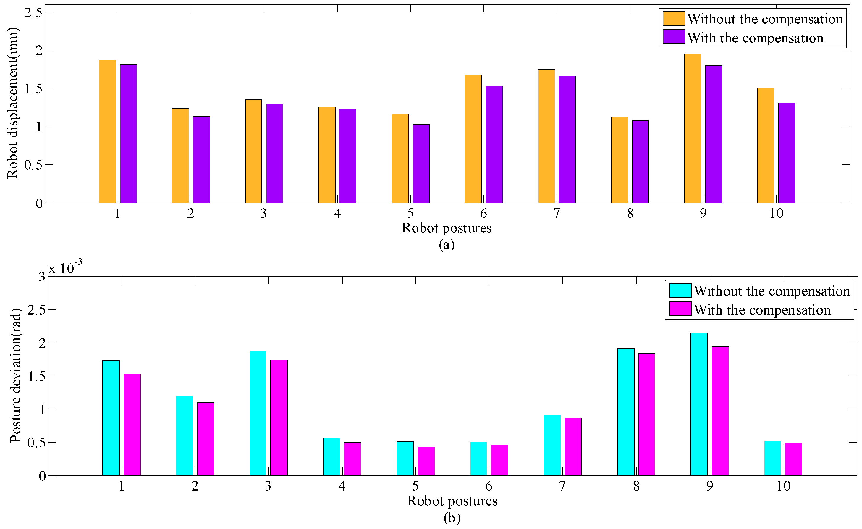
Figure 7a illustrates the position error of R1. The accuracy of the position has improved and the maximum position value is less than 1.81 mm.
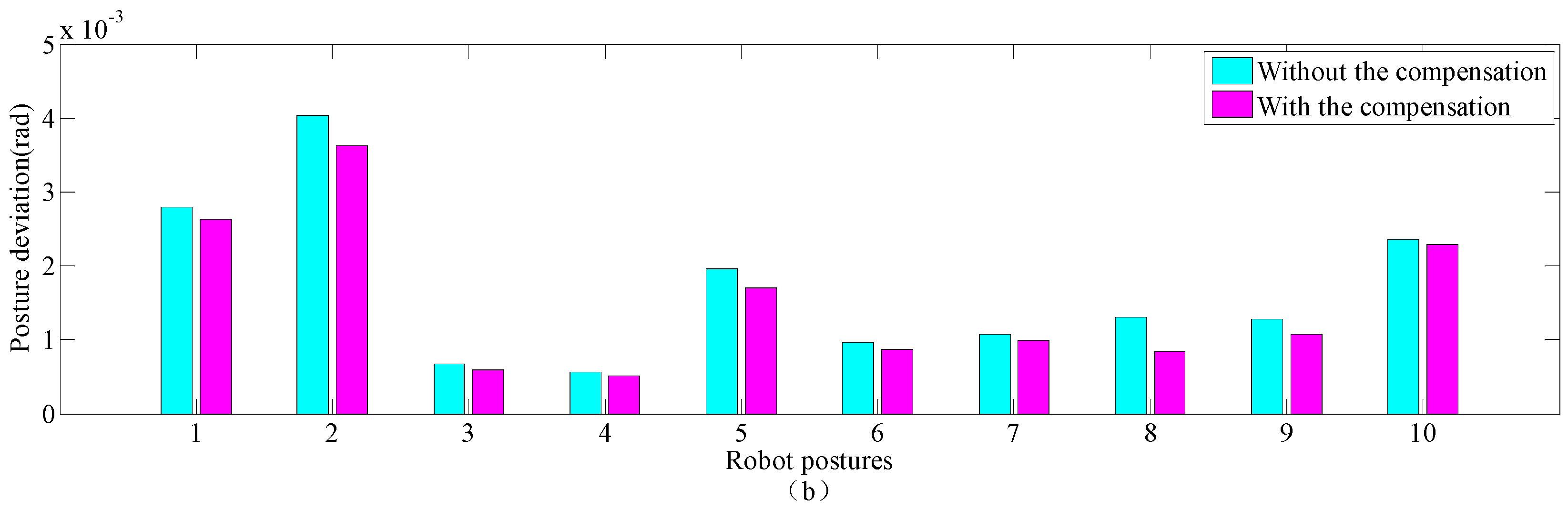
Figure 7b illustrates the orientation error of R1, and the maximum orientation value is less than 0.0019 rad.
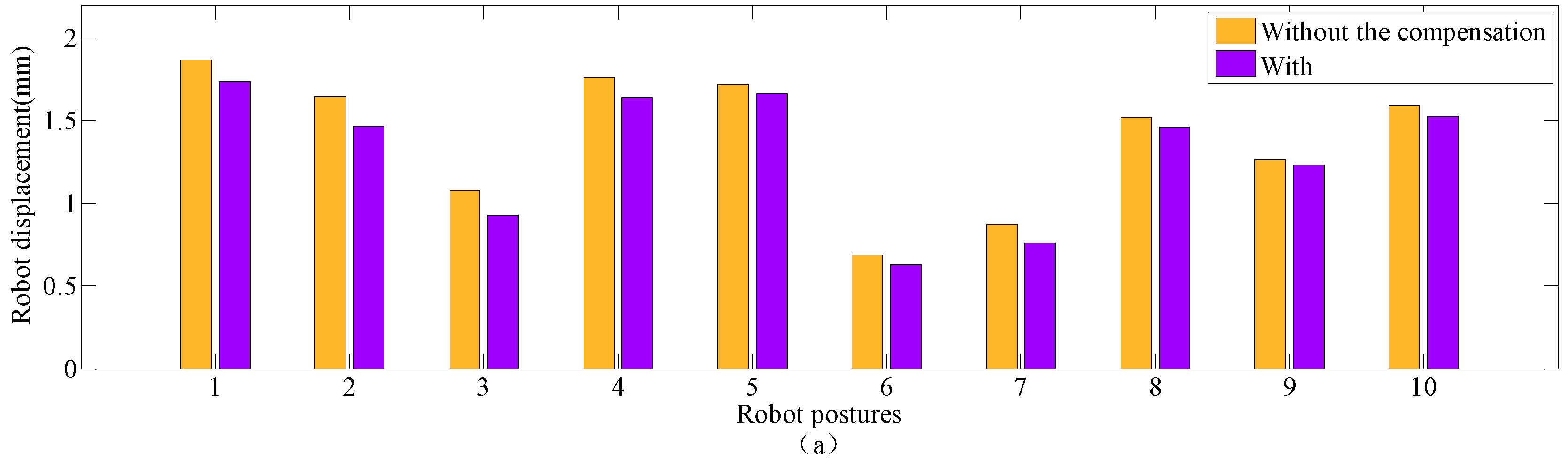
Figure 8a illustrates the position error of R2. The accuracy of the position has improved and the maximum position value is less than 1.72 mm.
Figure 8b illustrates the orientation errors of R2, and the maximum orientation value is less than 0.0037 rad.
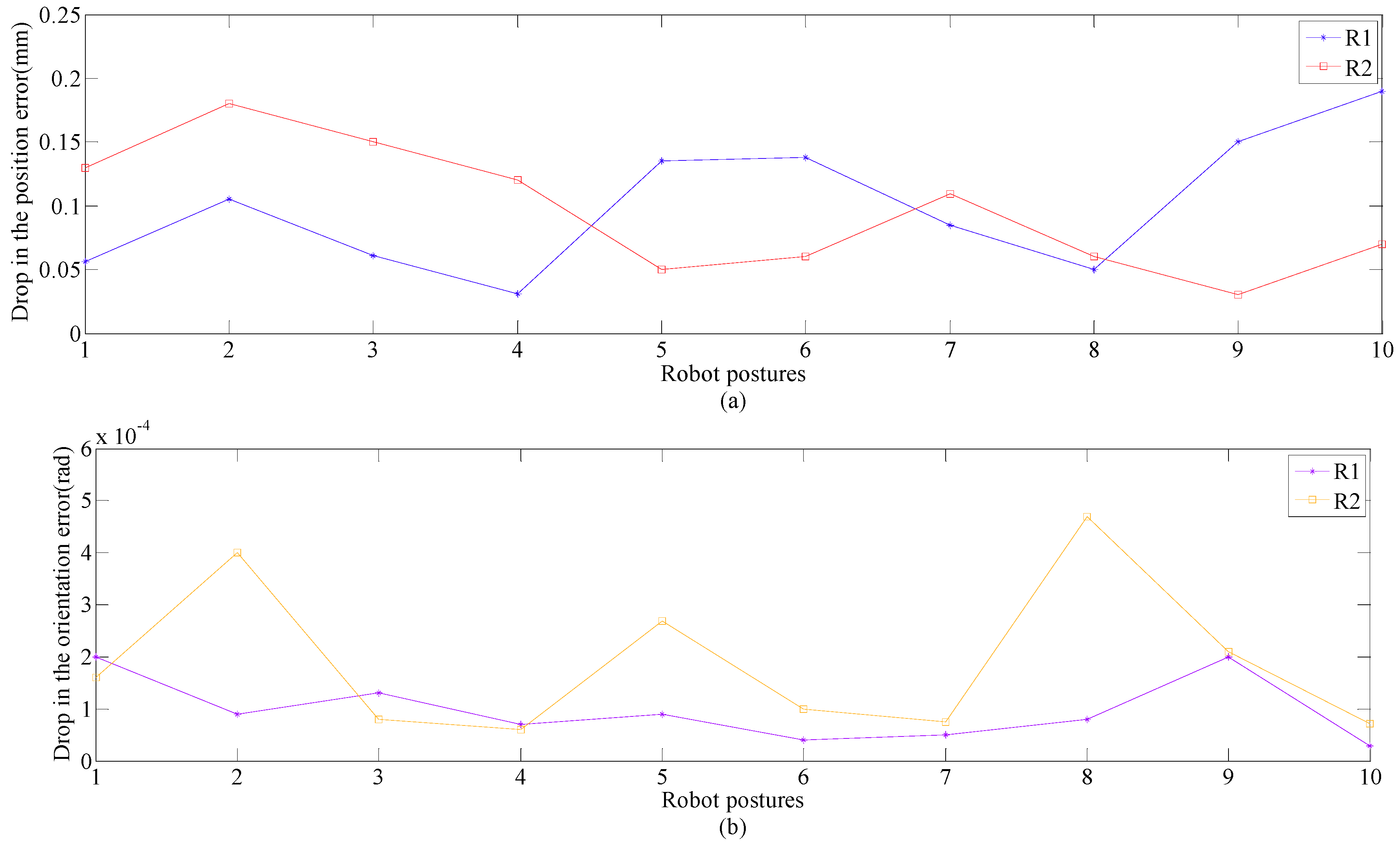
Figure 9 shows the drops in the position error and orientation error of the EE.
Figure 9a shows that the position error is better than the before, as expected after the calibration.
Figure 9b shows that the orientation error is better than the before, as expected after the calibration as well. The identification results show that the joint stiffness of the SDA5F robot was not very small, thus there were slight drops in the errors. Furthermore, the residual errors were caused mainly by the geometrical kinematic errors of the robot that were beyond the aspect of this paper. Nevertheless,
Figure 9 depicts the improvement of the accuracies of the EEs.
During the experiment, a carbide drill was used for the procedure, and the drill diameter was . The circuit board was mounted on the supporting side, which was R1, and the six-axis force sensor 1 measured the supporting forces and torques. The circuit board was in size. The target location of the drilling operation was chosen on the circuit board, and the feed rate was set manually. The location was important for the drilling operation, and the pose of the drilling EE was calculated based on the forward kinematic equation mentioned above. In addition, the pose error of the EE and the drill axis direction were important for the performance of the drilling operation, and the deformation compensation was added to the control loop of the robot controller. After the compensation, the location can be chosen precisely. The drill axis direction was perpendicular to the plane of the circuit board.
During the drilling operation, the velocity of the drill was set to about 0.001 mm/r manually in order to be a constant element, and the measurement can be concise during the drilling operation as the force sensors have high accuracy. The drilling EE mounted on six-axis force sensor 2 was drilling towards the circuit board, and the
z-axis of R1 was parallel to the drill axis direction. Specifically, the drilling EE was moving while the R1 was holding steady during the procedure. The force sensor 2 was measuring the forces and torques during the drilling of the circuit board. The force sensor 1 measured the supporting forces and torques of R1 at the same time. Furthermore, the force sensors measured the force and torque until the drill penetrated the circuit board. In addition, the forces and torques were measured before and after the compensation during the experiment. The errors of positions and orientations caused by the deformation before and after the compensation resulted in different performances of forces and torques applied to the circuit board and drilling EE, respectively. When the drilling EE pressed the surface of the circuit board, the absolute value of force along the drill axis direction was increasing. At the same time, the absolute value of the force along the
z-axis of the EE of R2 was increasing. After the drill penetrated the circuit board, the absolute value of forces was decreasing.
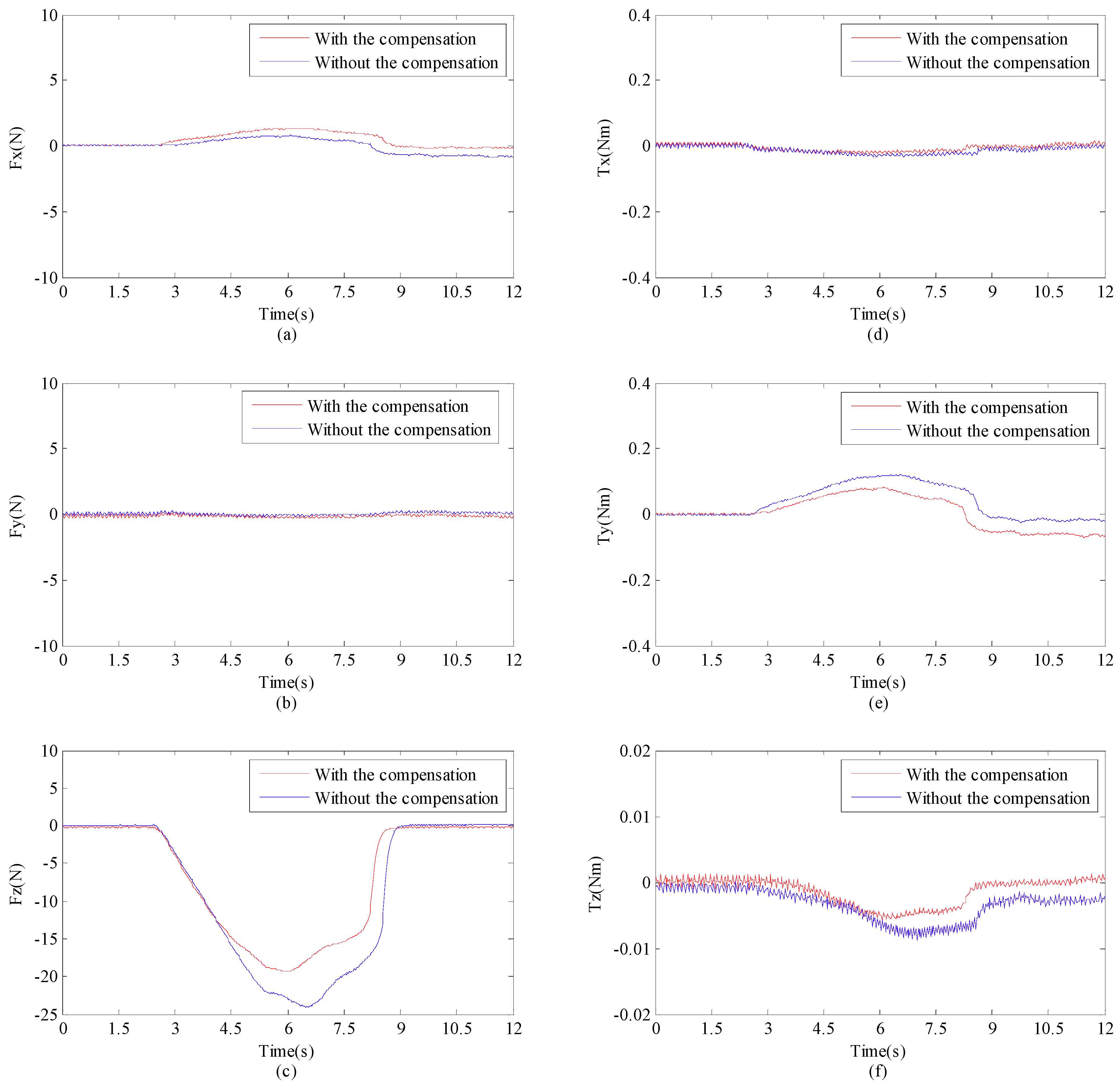
Figure 10 shows the force and torque curves of R1 before and after the compensation.
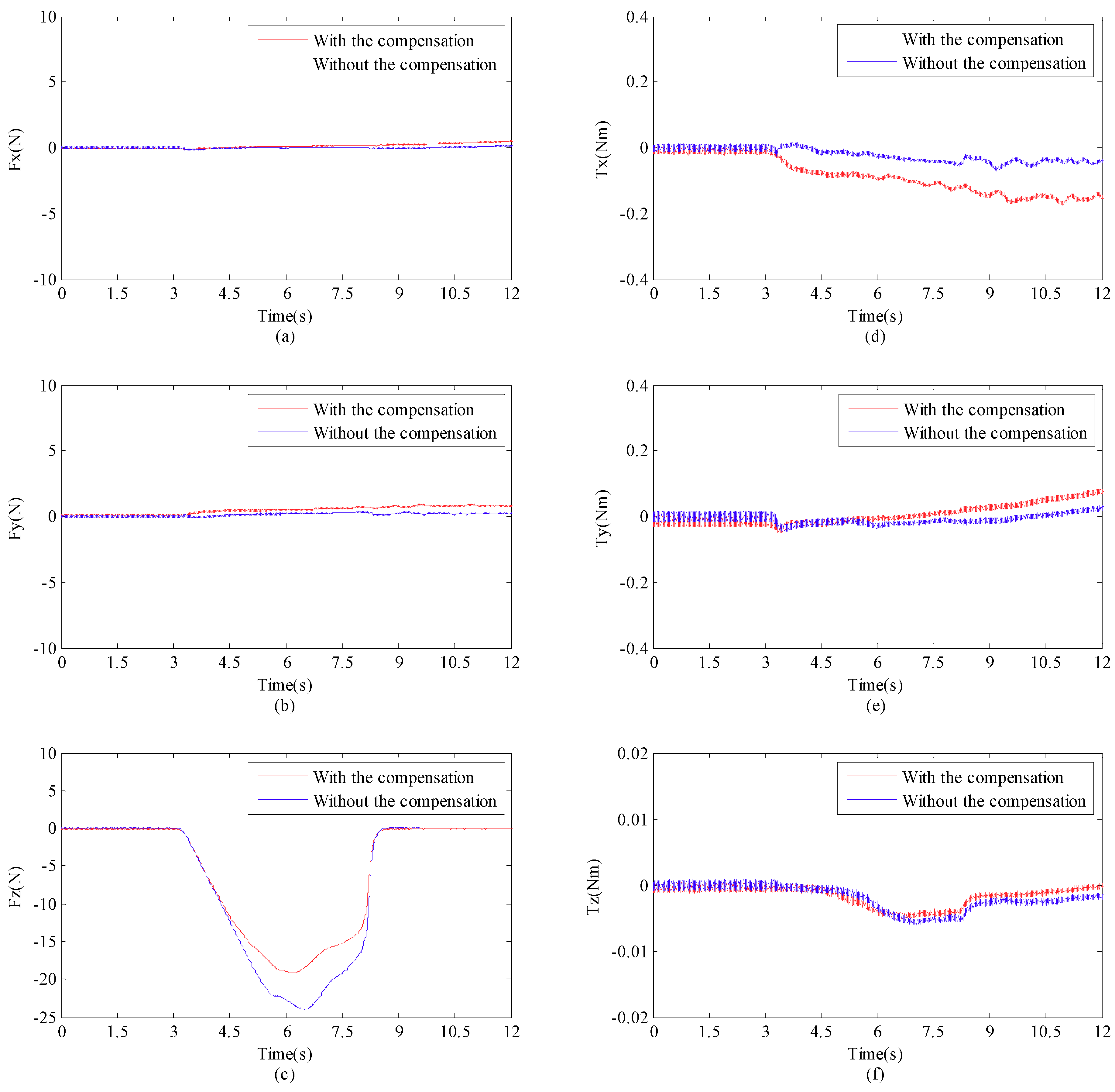
Figure 11 shows the force and torque curves of R2 before and after the compensation.
The red curve in
Figure 10c is the force Fz along the drill axis which is the feed direction, and the absolute value of Fz is the biggest one among Fx, Fy, and Fz. The Fz with the compensation is smaller than the one without the compensation, as the drill axis direction is controlled perpendicularly, and the other two forces are smaller than those without the compensation. This is because these two forces are used to cut the material and the bigger deformation would cause bigger forces and torques in their directions. Furthermore, the torques Tx, Ty, and Tz have the similar trend of changes. However, the absolute values of torques Tx, Ty, and Tz are small because the corresponding forces are small especially with the deformation compensation.
Figure 11 shows that the forces and torques applied to the EE of R2 have the similar trend of changes, because there are interaction forces between the two arms during the experiment. Nevertheless, the absolute values of forces and torques shown in
Figure 10 are not the same like those in
Figure 11. This is mainly because the forces and torques represented in the frame of six-axis force sensor 1 are different with those in the frame of six-axis force sensor 2 and the measurement noise. However, the force Fz measured by the six-axis force sensor 1 is closed to the force Fz measured by the six-axis force sensor 2, and this is because the drill axis is near perpendicular to both z-axes of the two force sensors.
Figure 10c shows that the maximum absolute value of force Fz is at 6.5 s due to the resistance changing after the penetration of the circuit board.
Figure 11c shows that the force Fz has a similar maximum value as well. The forces and torques were controlled more precisely after the deformation compensation of the industrial robot. As shown in these figures, the proposed stiffness modeling and deformation compensation algorithm are effective and can be used for further study.


