Integrated High-Performance Platform for Fast Query Response in Big Data with Hive, Impala, and SparkSQL: A Performance Evaluation


Abstract
:1. Introduction
2. Related Work
2.1. Literature Review and Motivation
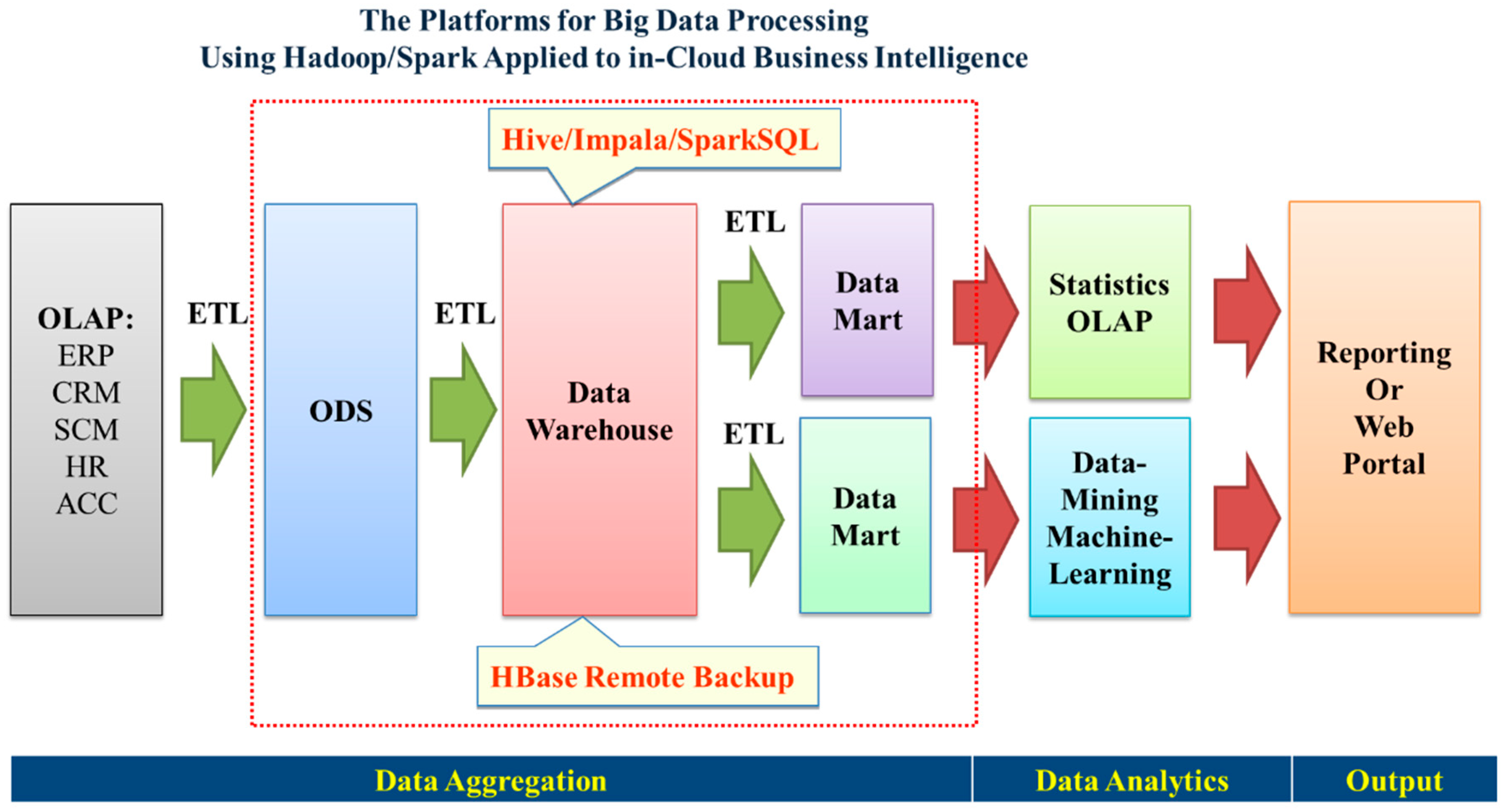
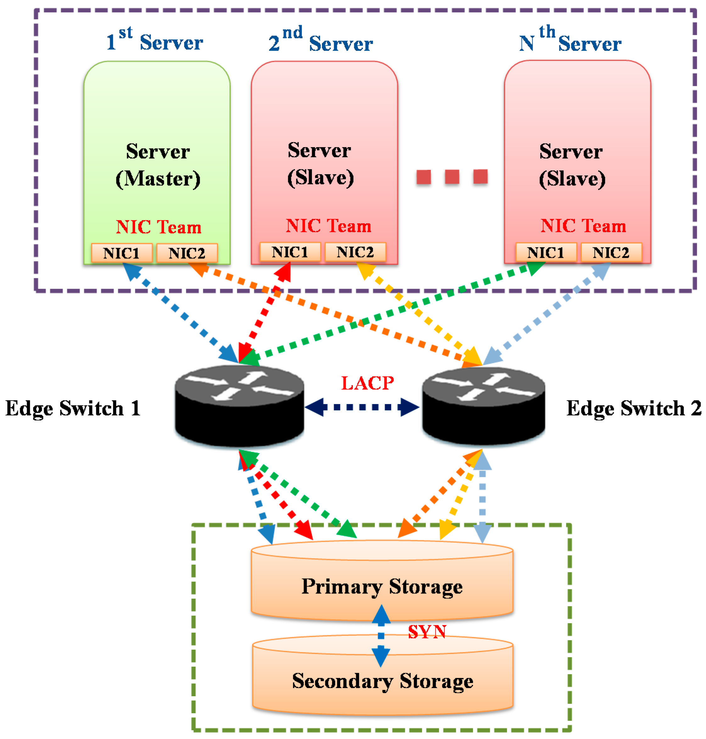
2.2. Computing Environment
2.3. Key Computing Components
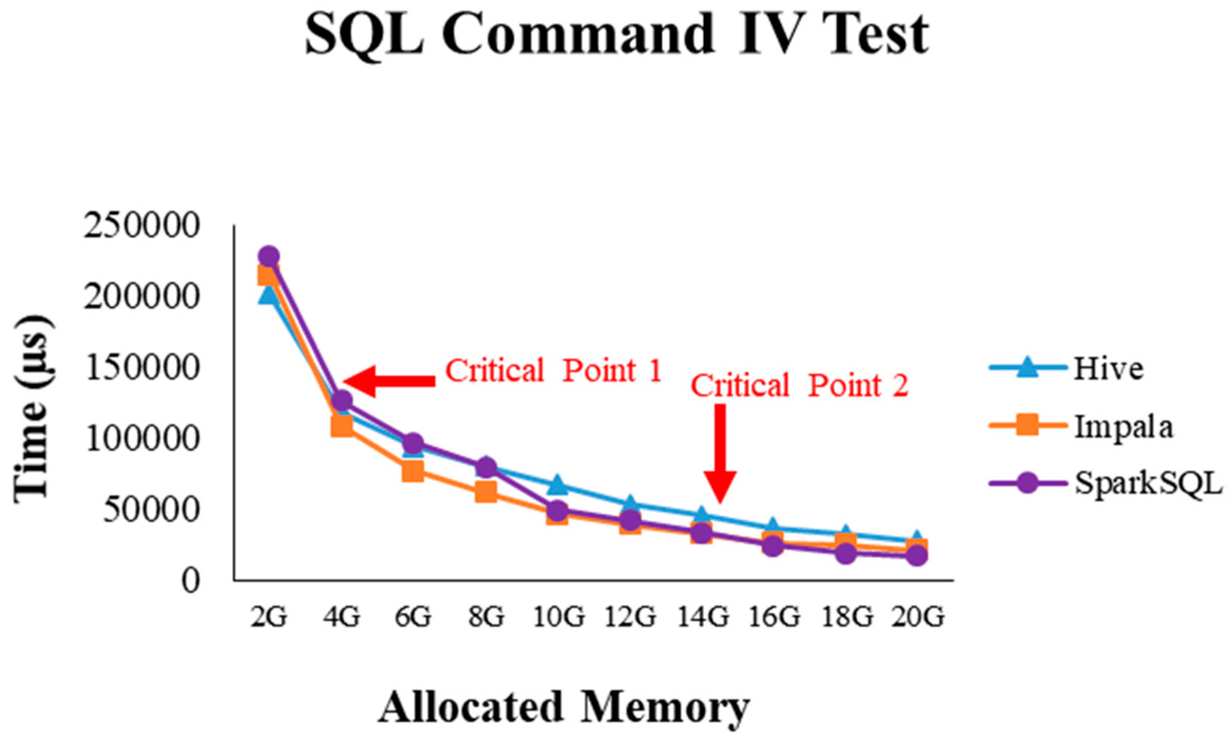
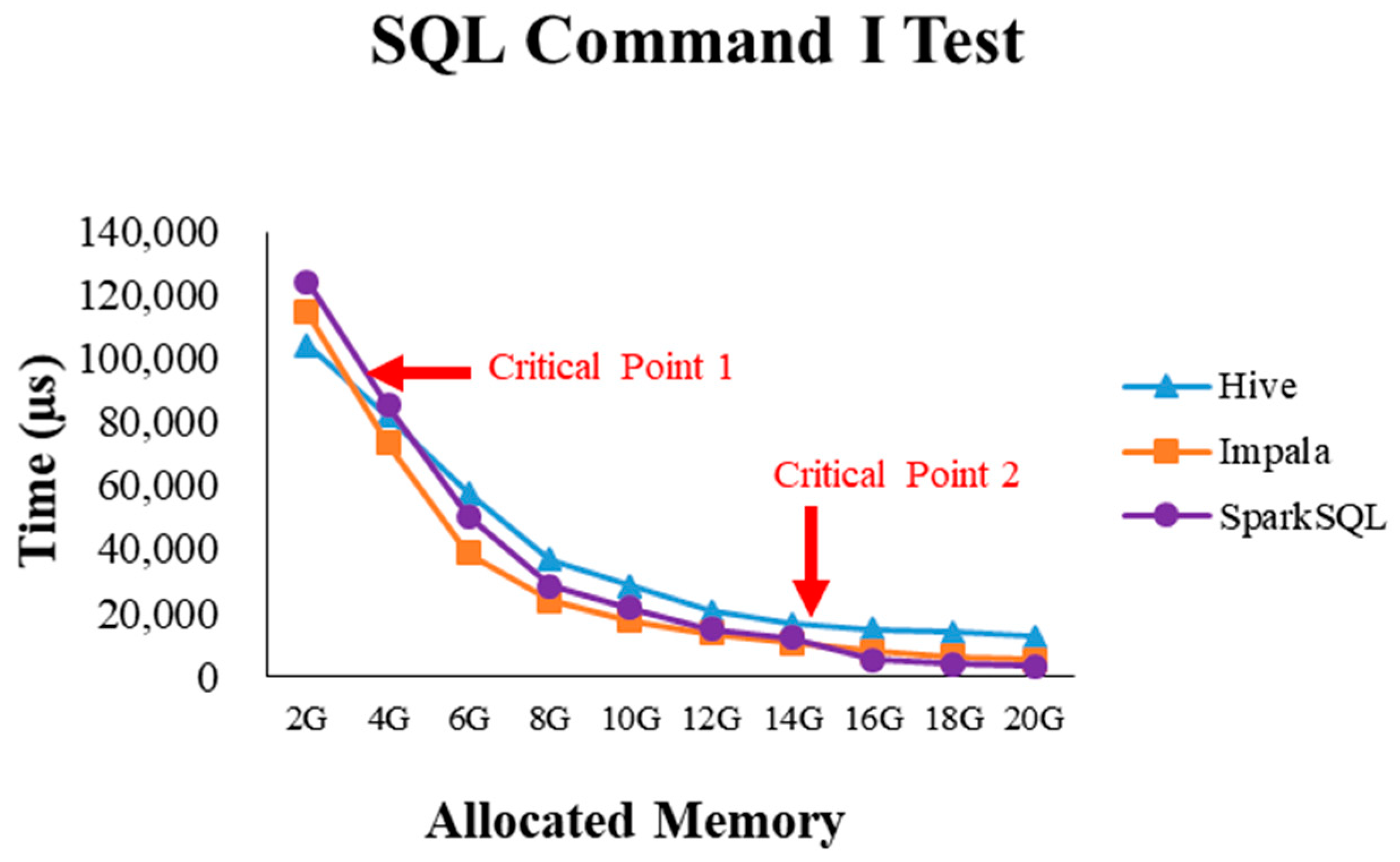
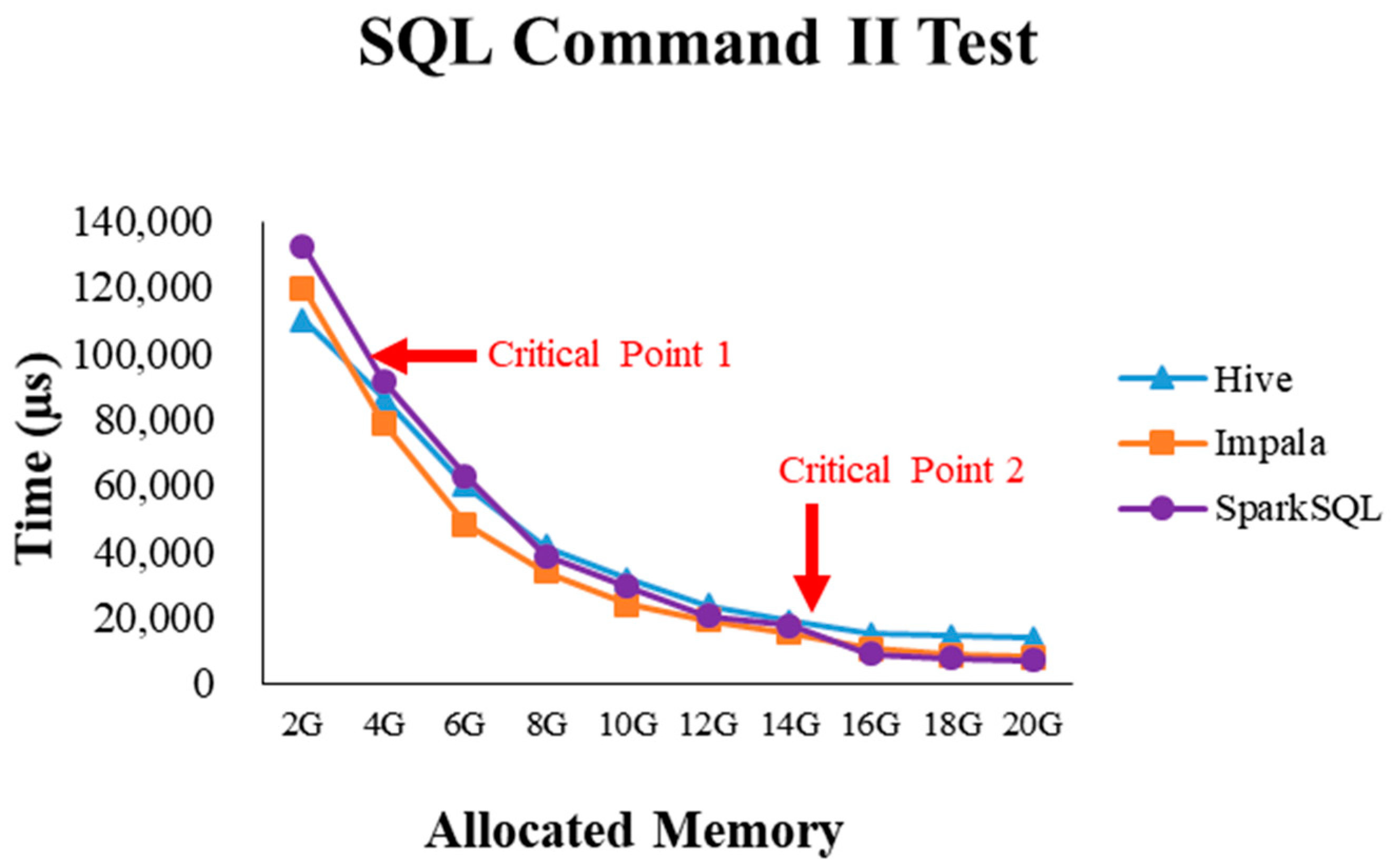
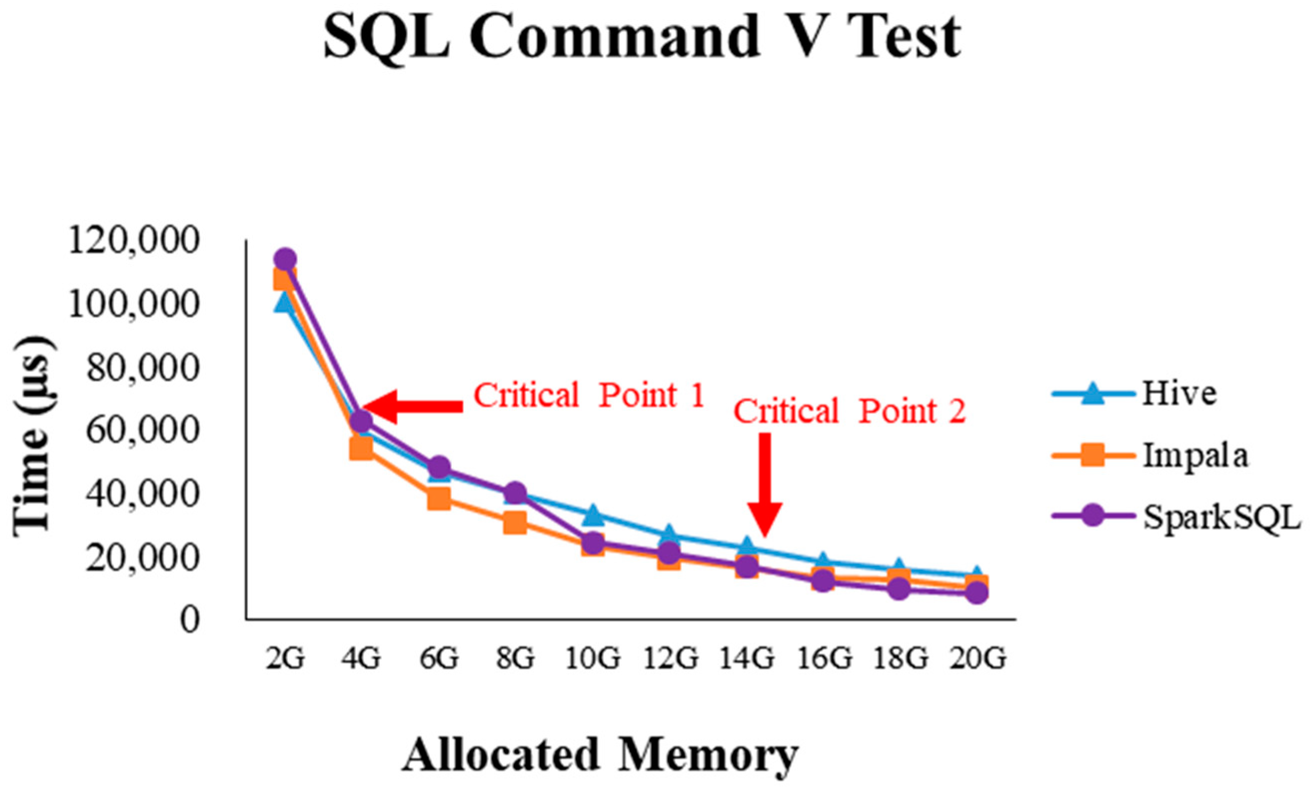
2.4. Critical Point Discovery
3. System Implementation and Performance Evaluation
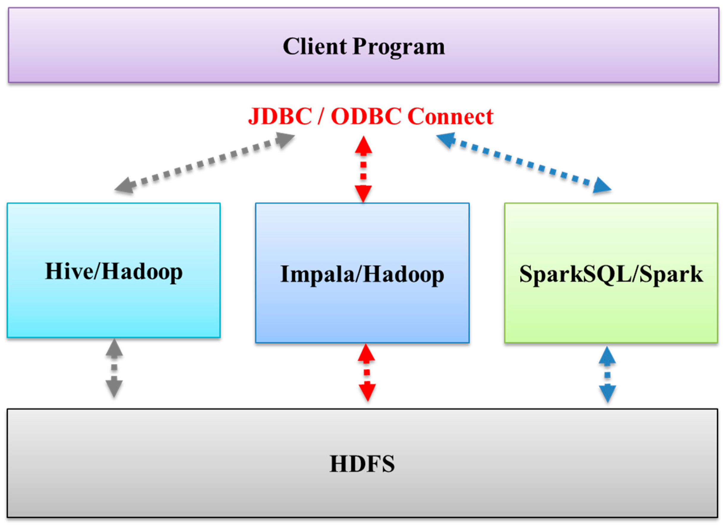
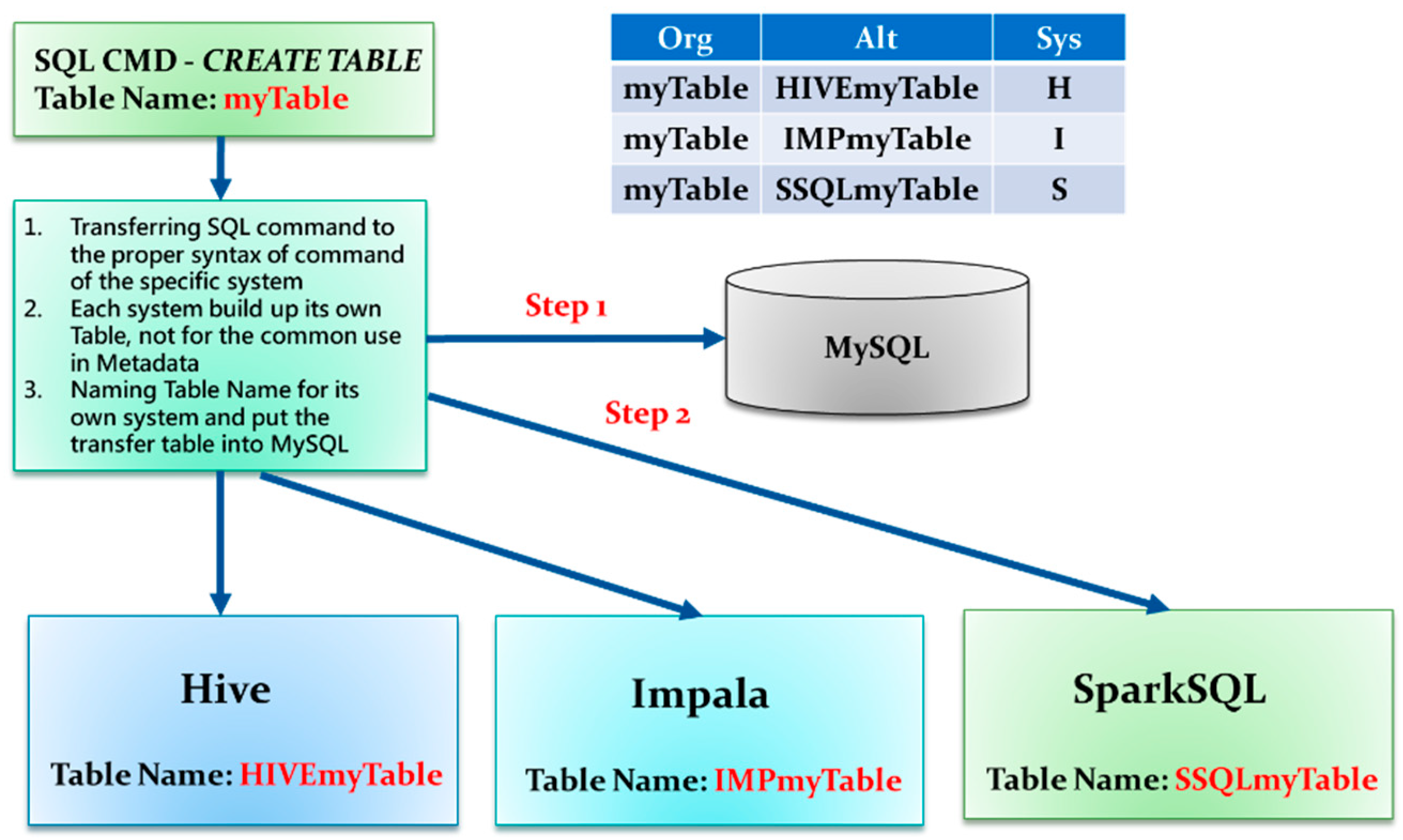
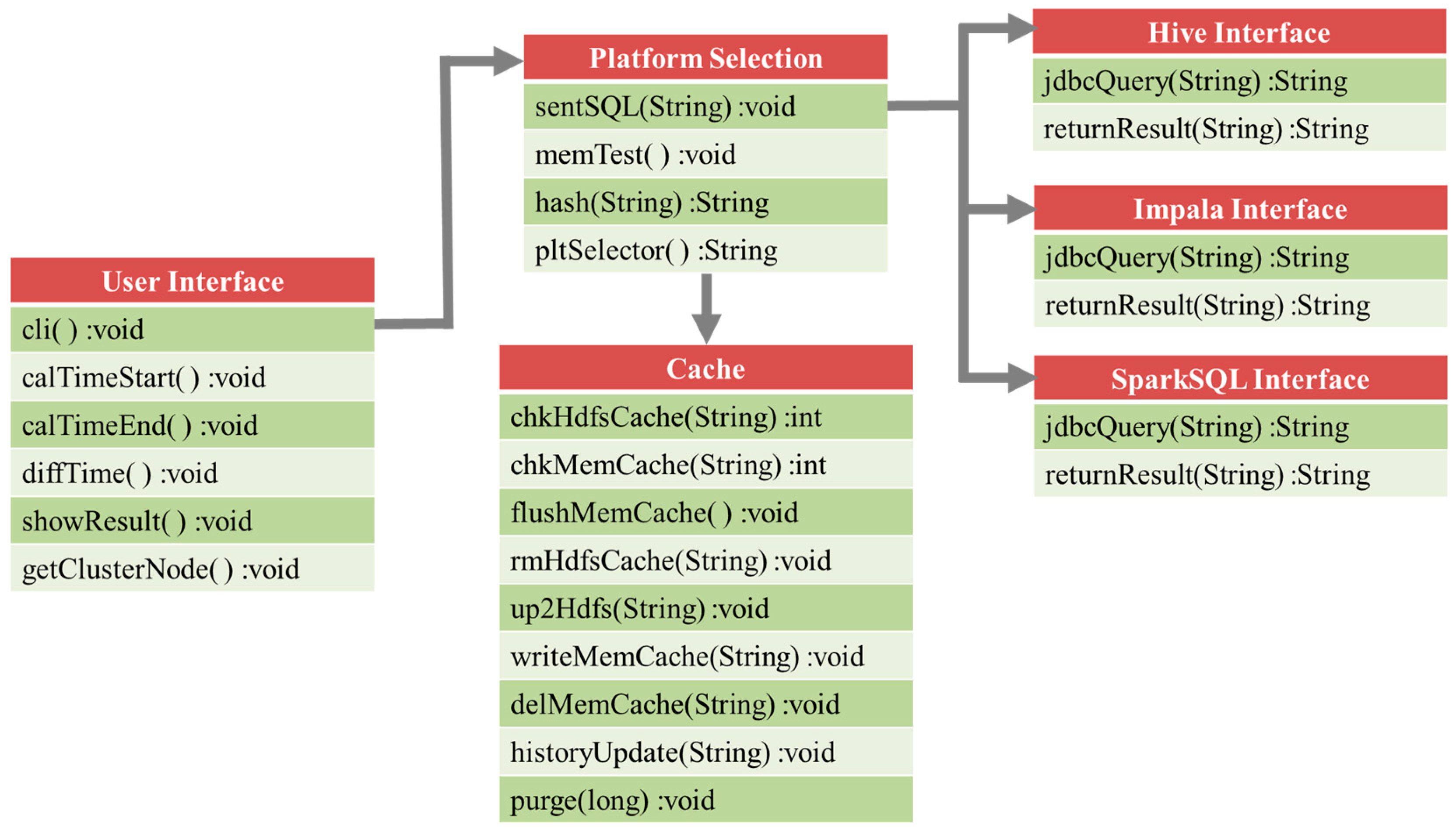
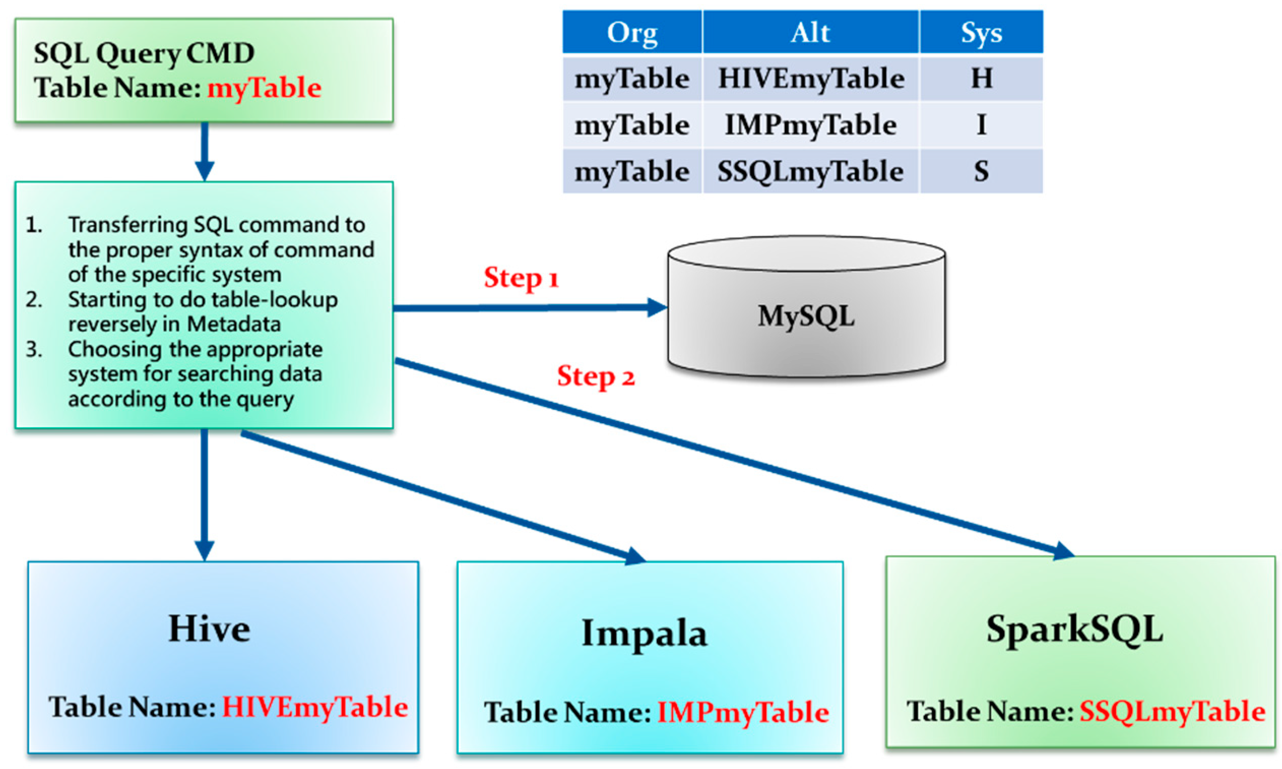
3.1. Multi-System Compatible Solution
3.2. Platform Selection
| Algorithm 1. Platform selection algorithm (PSA) |
INPUT: Job u from command list LC. OUTPUT: Appropriate platform assigned set assign(u, ej).
|
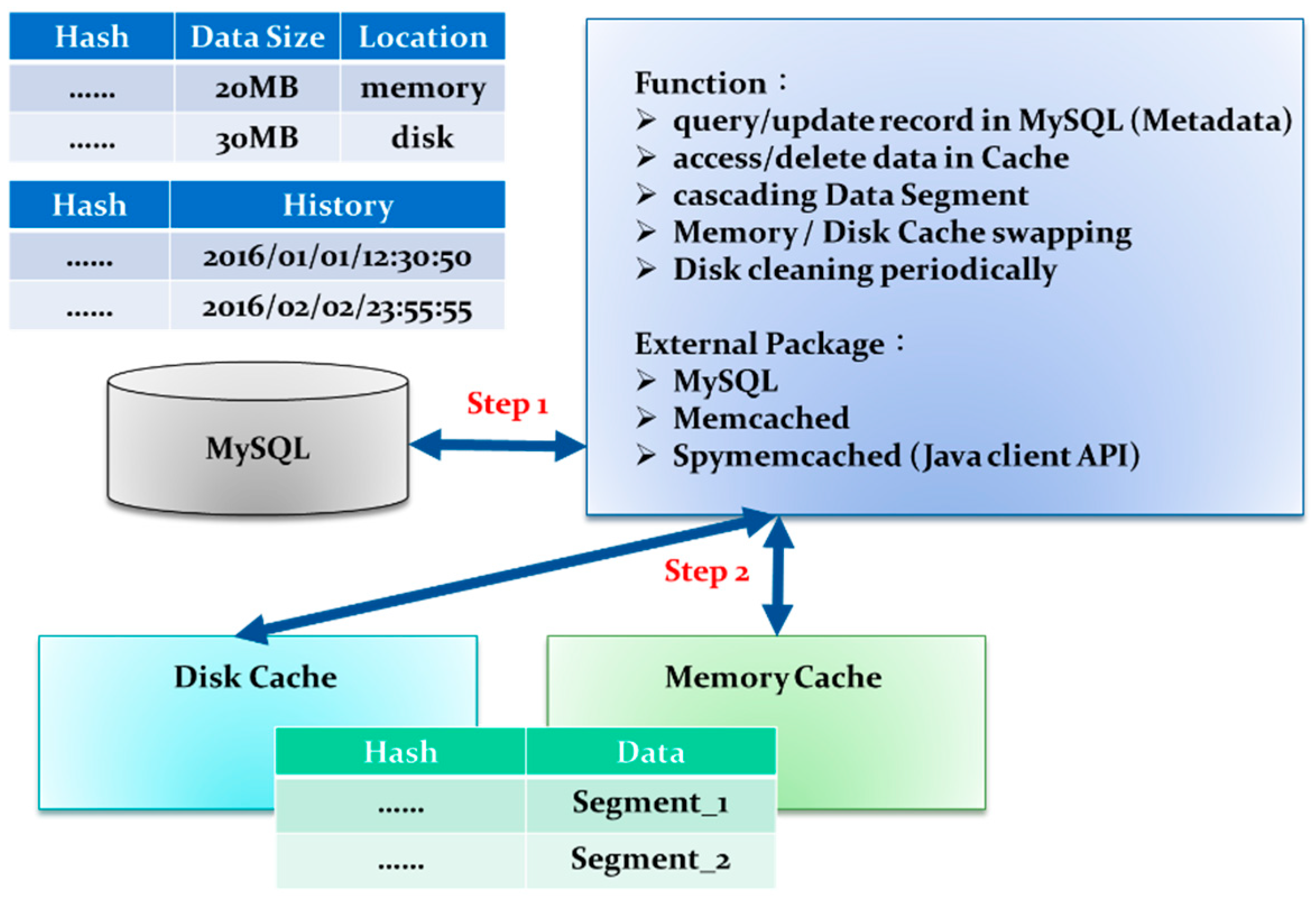
3.3. In-Memory Cache and In-Disk Cache
| Algorithm 2. Delete out-of-date data in the memory cache |
Input: FHm, Hm, Hmr. Output: Updated memory cache record Hmr.
|
| Algorithm 3. Delete out-of-date file in the disk cache |
Input: FHd, Hd, Hdr. Output: Updated disk cache record Hdr.
|
| Algorithm 4. Add up-to-date data to the memory cache |
Input: FHm, Hm, Hmr. Output: Updated memory cache record Hmr.
|
| Algorithm 5. Add up-to-date data to the disk cache |
Input: FHd, Hd, Hdr. Output: Updated memory cache record Hdr.
|
| Algorithm 6. Visit current data (hit or miss) in the memory cache |
Input: Di+ Hm, Hmr. Output: result.
|
| Algorithm 7. Visit current data (hit or miss) in the disk cache |
Input: Di+ Hd, Hdr. Output: result.
|
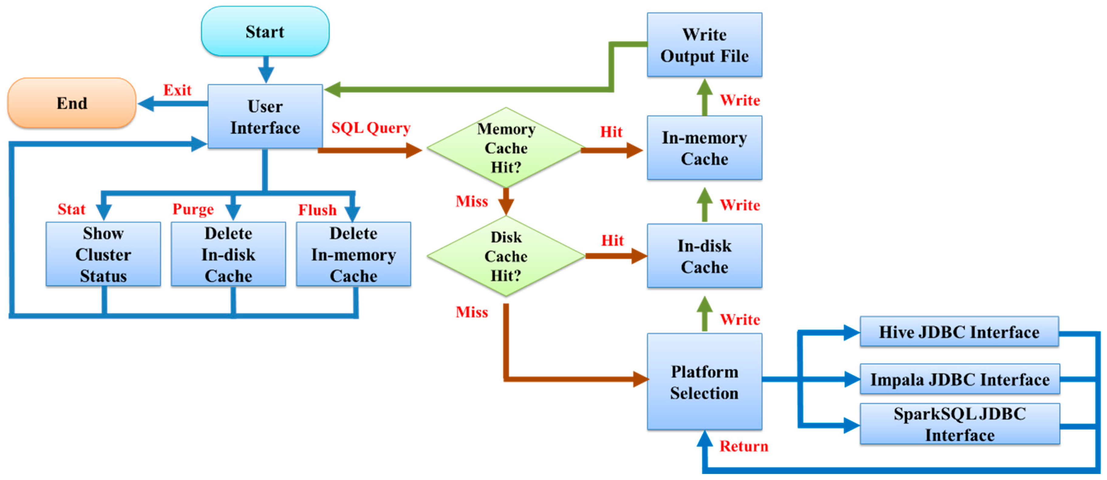
3.4. Execution Procedure
3.5. Performance Index
4. Experimental Results and Discussion
4.1. Experimental Environment in Case 1
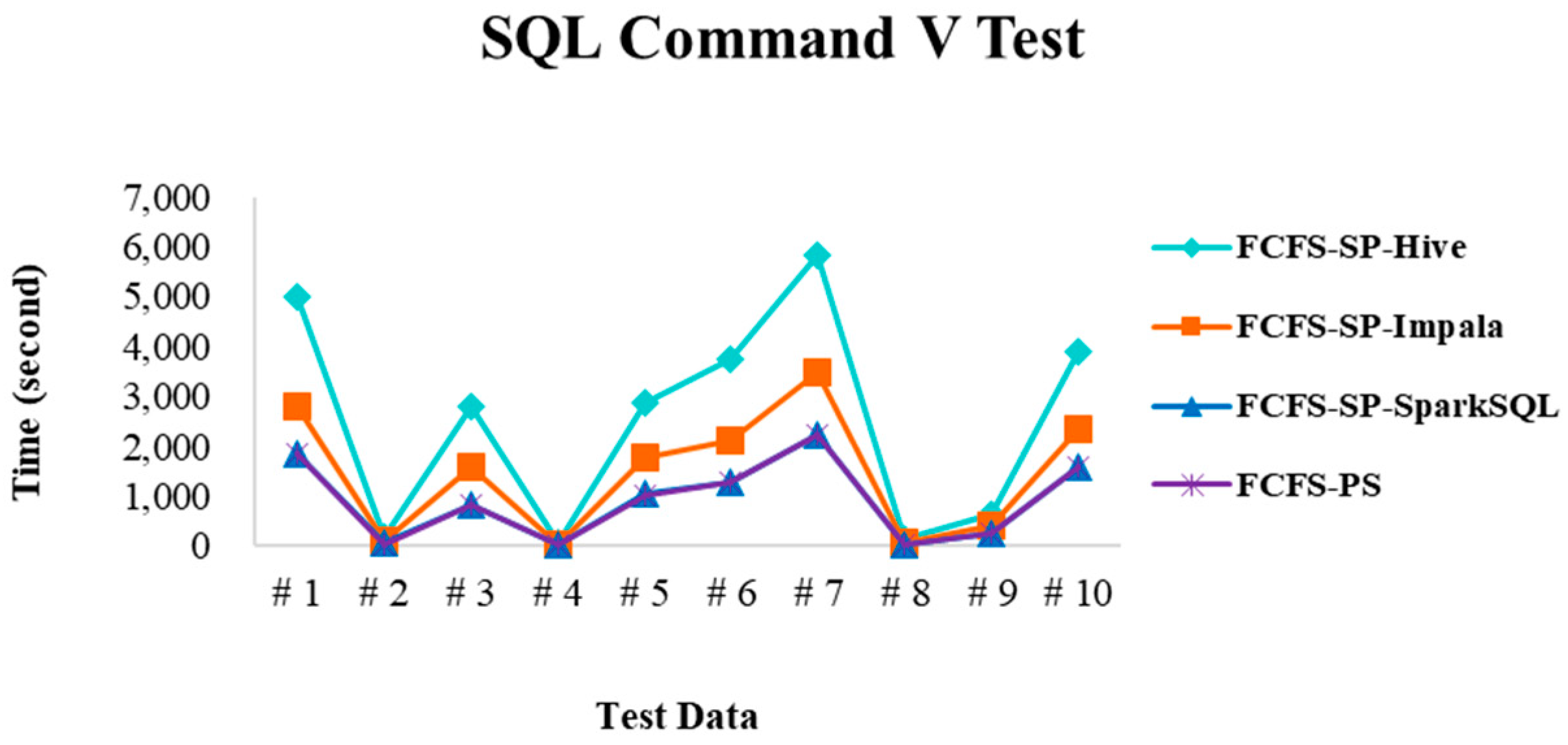
4.2. Experimental Results in Case 1
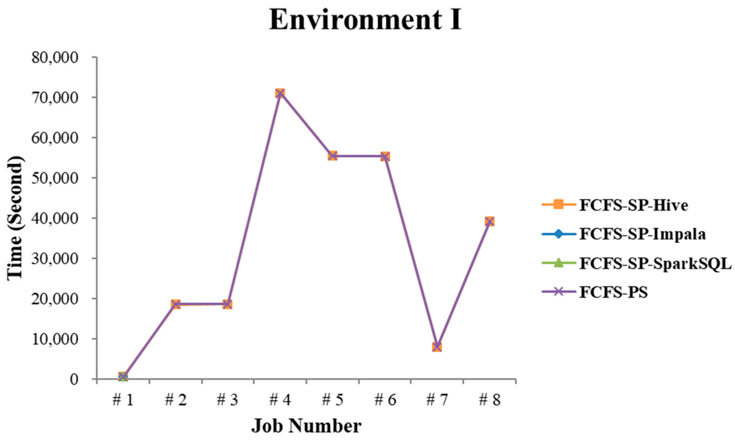
4.2.1. Test Environment I
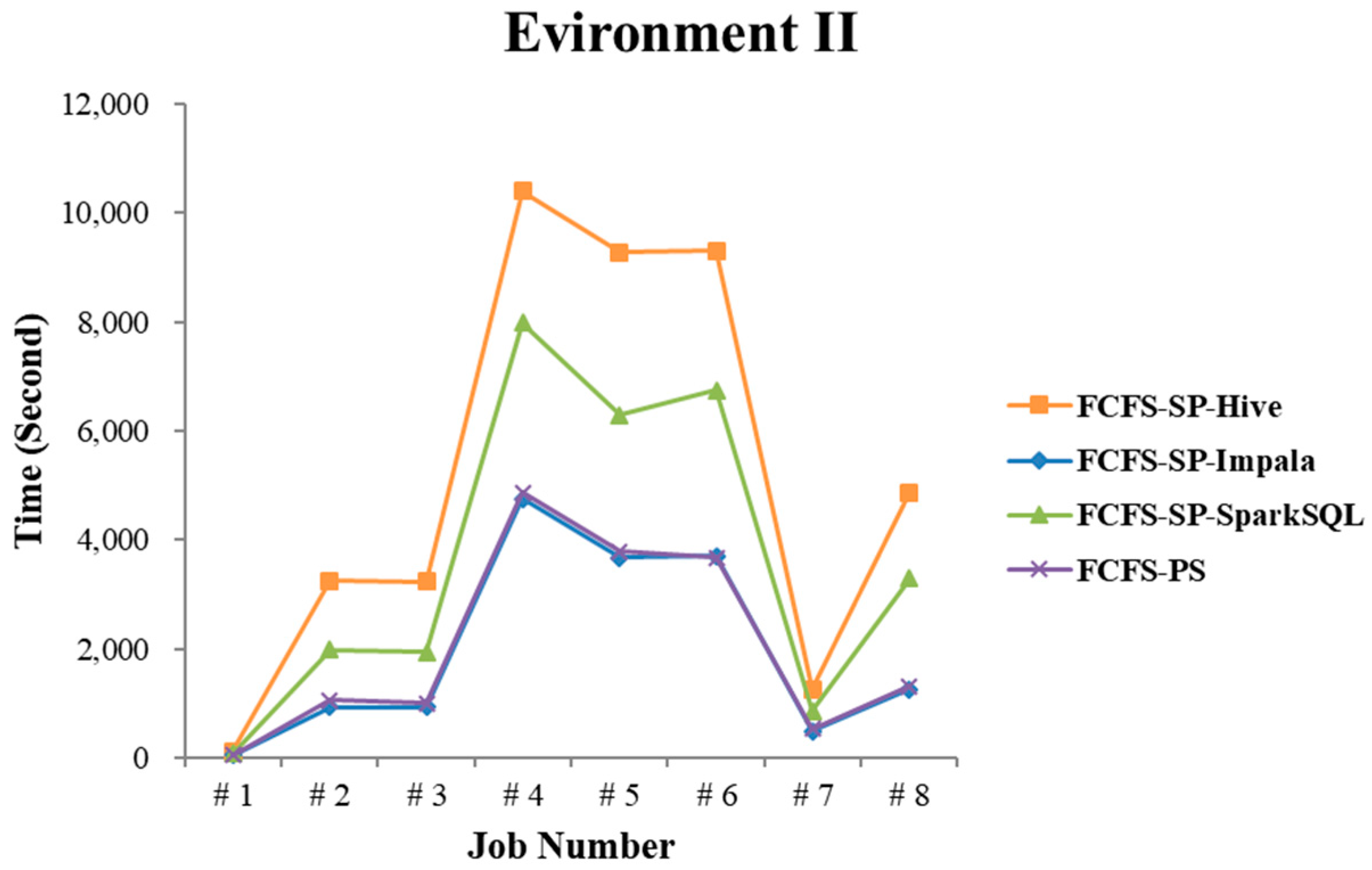
4.2.2. Test Environment II
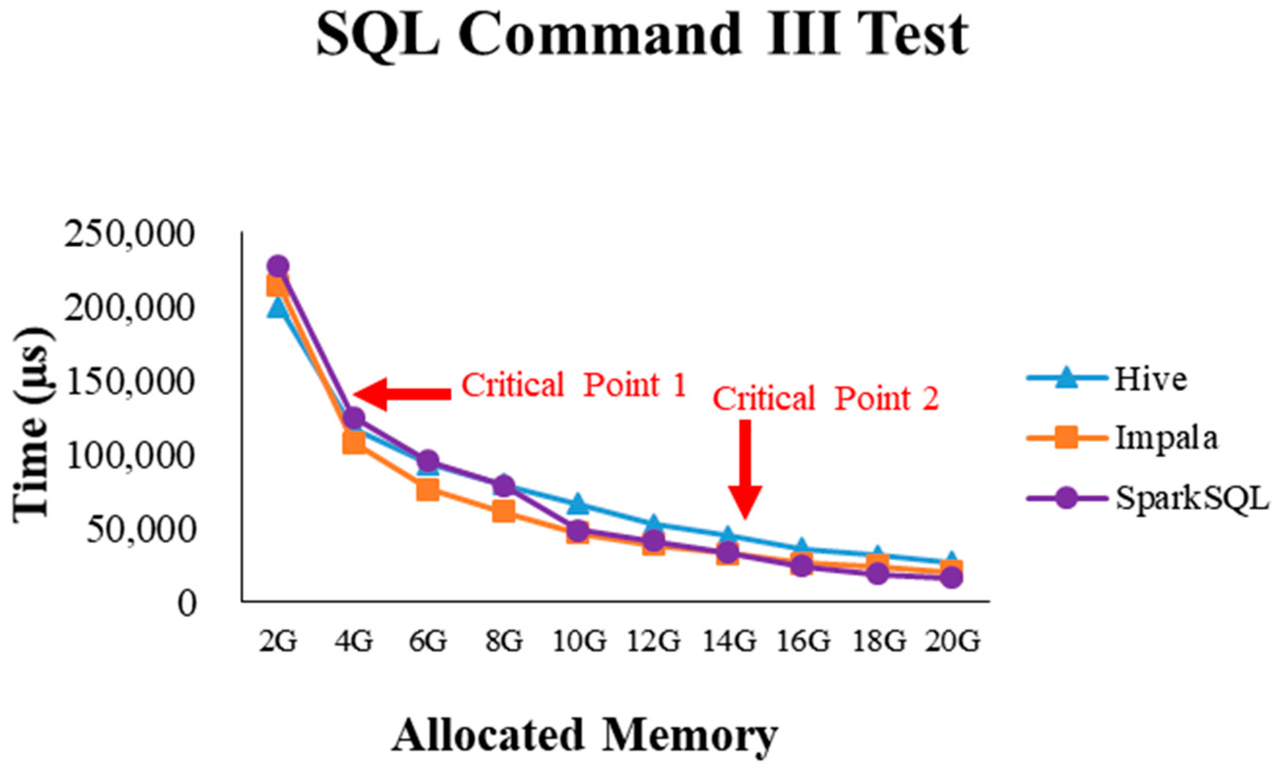
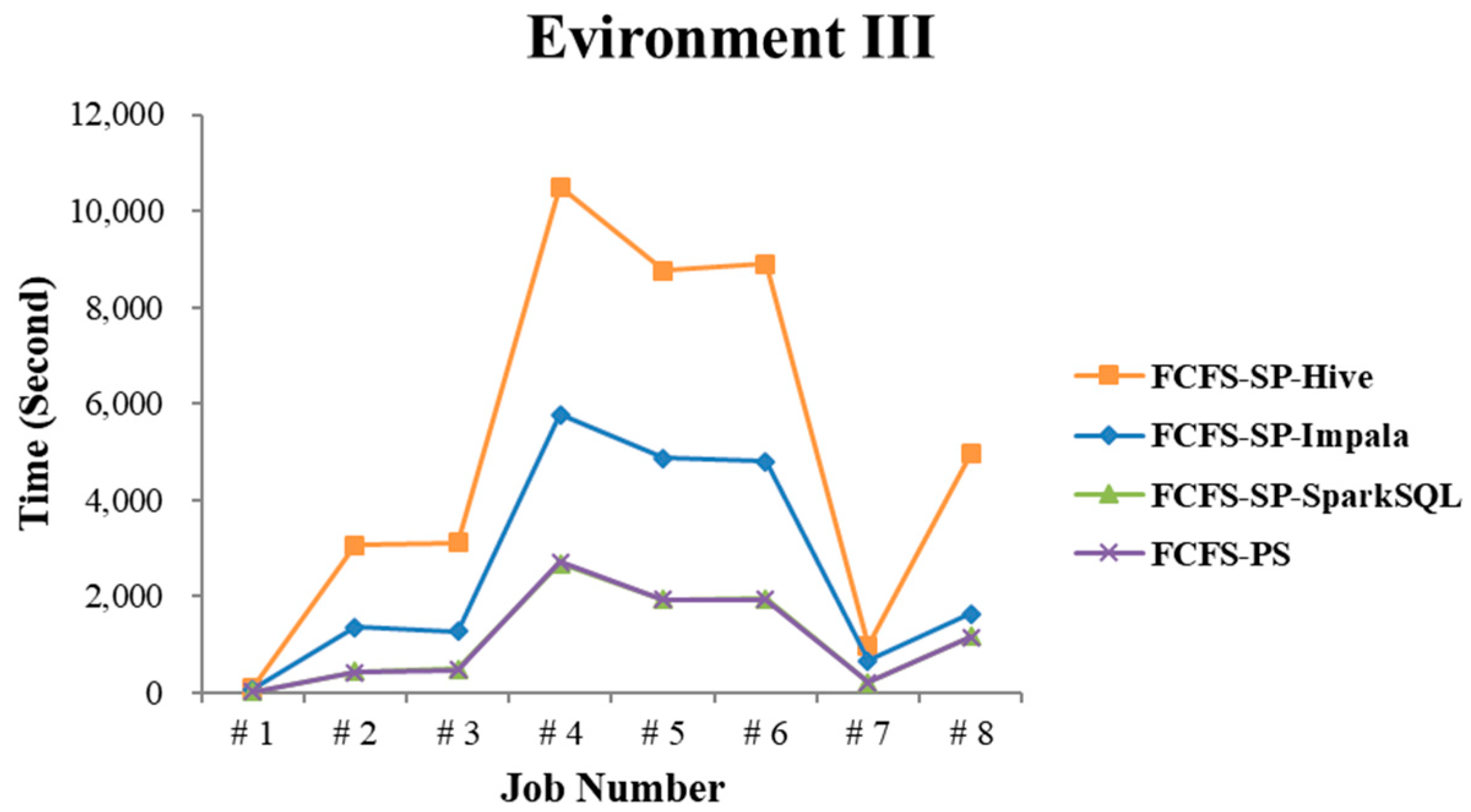
4.2.3. Test Environment III
4.2.4. Performance Evaluation
4.3. Experimental Environment in Case 2
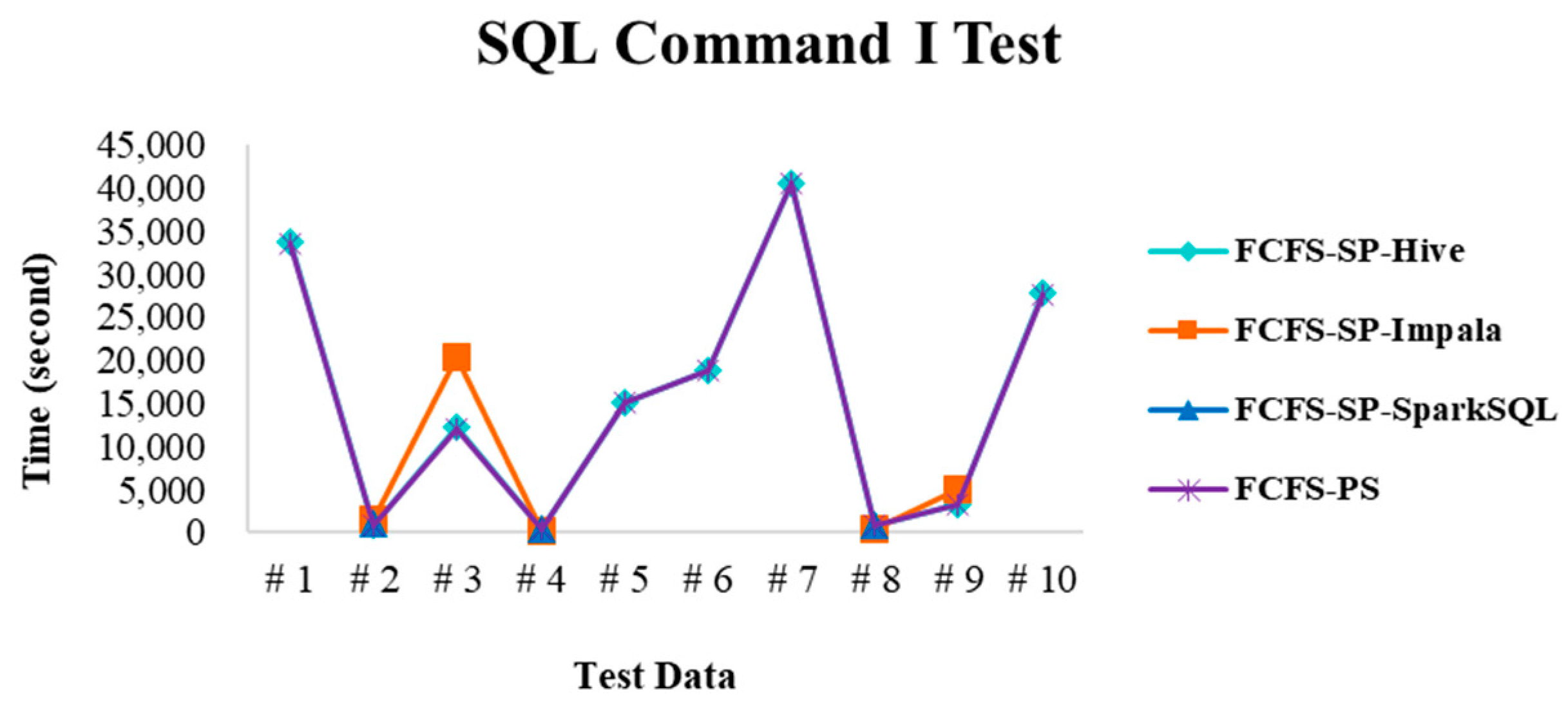
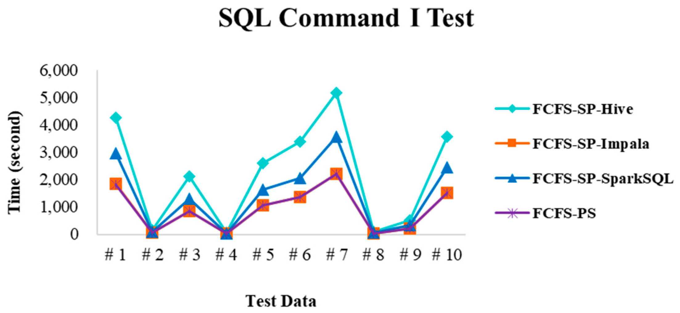
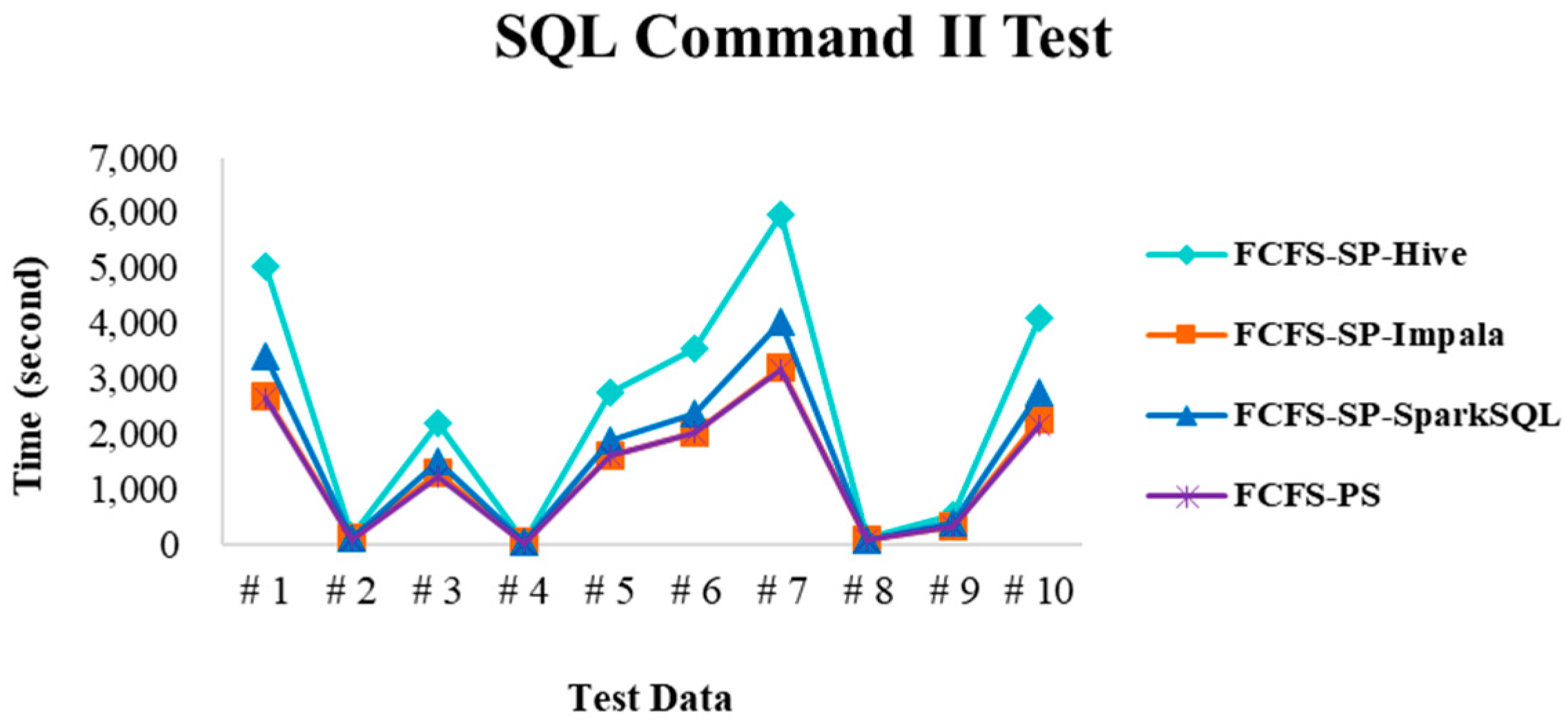
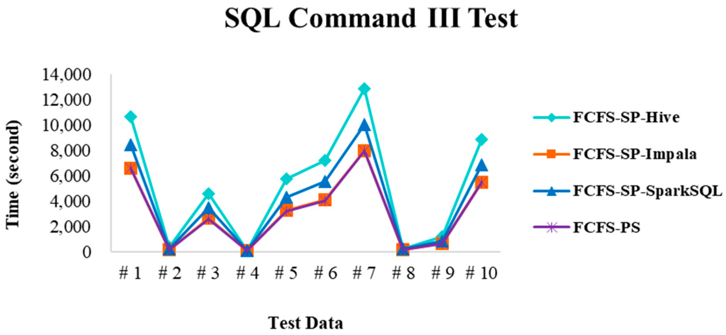
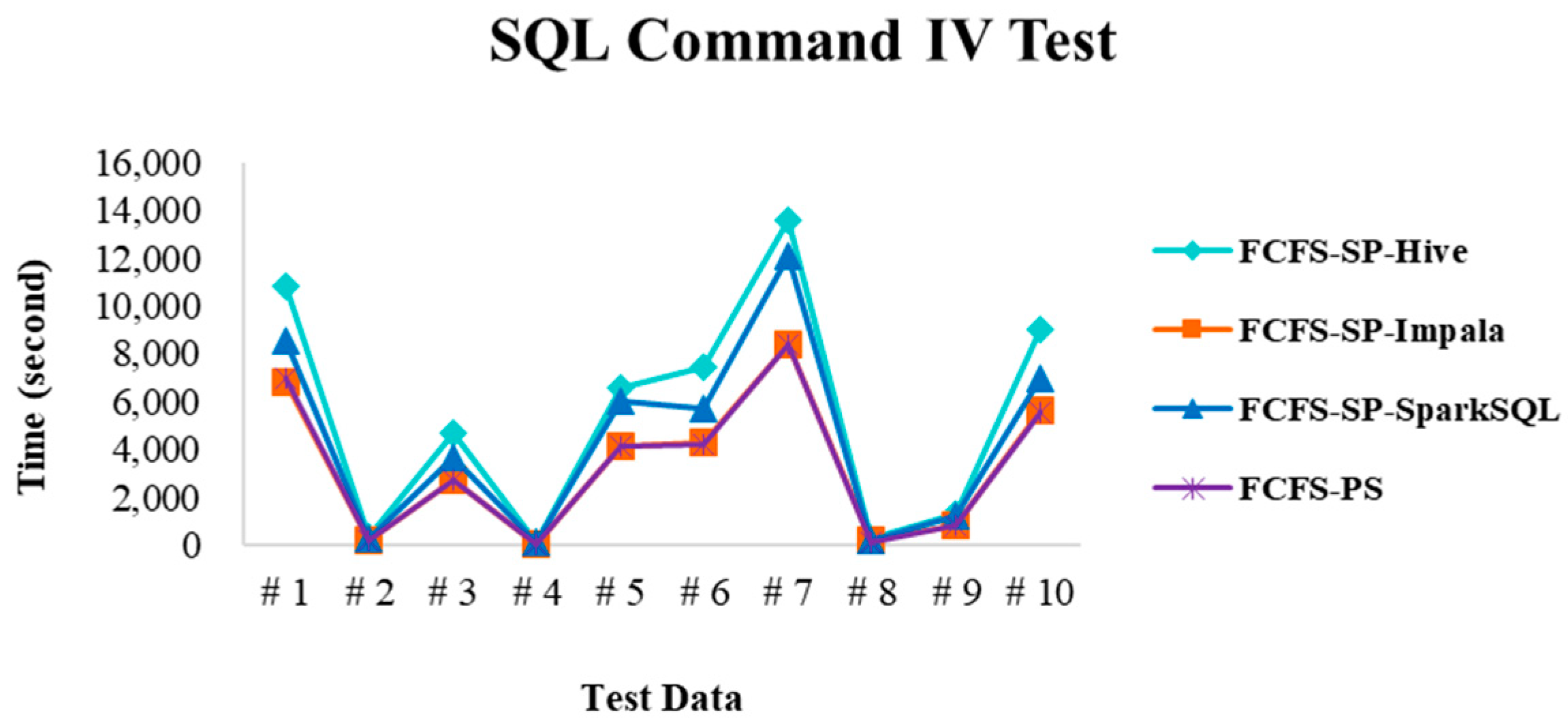
4.4. Experimental Results in Case 2
4.5. Discussion
5. Conclusions
Author Contributions
Funding
Conflicts of Interest
References
- Almgren, K.; Kim, M.; Lee, J. Extracting Knowledge from the Geometric Shape of Social Network Data Using Topological Data Analysis. Entropy 2017, 19, 360. [Google Scholar] [CrossRef]
- Fan, S.; Lau, R.Y.; Zhao, J.L. Demystifying Big Data Analytics for Business Intelligence through the Lens of Marketing Mix. Big Data Res. 2015, 2, 28–32. [Google Scholar] [CrossRef]
- Wixom, B.; Ariyachandra, T.; Douglas, D.E.; Goul, M.; Gupta, B.; Iyer, L.S.; Turetken, O. The Current State of Business Intelligence in Academia: The Arrival of Big Data. Commun. Assoc. Inf. Syst. 2014, 34, 1–13. [Google Scholar]
- Thusoo, A.; Sarma, J.S.; Jain, N.; Shao, Z.; Chakka, P.; Anthony, S.; Murthy, R. Hive: A Warehousing Solution over A Map-Reduce Framework. Proc. VLDB Endow. 2009, 2, 1626–1629. [Google Scholar] [CrossRef]
- Liu, T.; Margaret, M. Impala: A Middleware System for Managing Autonomic, Parallel Sensor Systems. ACM Sigplan Not. 2003, 38, 107–118. [Google Scholar] [CrossRef]
- Yadav, R. Spark Cookbook; Packt Publishing Ltd.: Birmingham, UK, 2015. [Google Scholar]
- Shvachko, K.V. Apache Hadoop: The Scalability Update. Login Mag. USENIX 2011, 36, 7–13. [Google Scholar]
- Zaharia, M.; Chowdhury, M.; Das, T.; Dave, A.; Ma, J.; Mccauley, M.; Stoica, I. Fast and Interactive Analytics over Hadoop Data with Spark. Login Mag. USENIX 2012, 37, 45–51. [Google Scholar]
- Borthakur, D. The Hadoop Distributed File System: Architecture and Design. Hadoop Proj. Website 2007, 11, 21. [Google Scholar]
- Dean, J.; Ghemawat, S. MapReduce: Simplified Data Processing on Large Clusters. Commun. ACM 2008, 51, 107–113. [Google Scholar] [CrossRef]
- Chang, F.; Dean, J.; Ghemawat, S.; Hsieh, W.C.; Wallach, D.A.; Burrows, M.; Chandra, T.; Fikes, A.; Gruber, R.E. Bigtable: A Distributed Storage System for Structured Data. In Proceedings of the 2006 USENIX Symposium on Operating Systems Design and Implementation (OSDI), Seattle, WA, USA, 6–8 November 2006; pp. 205–218. [Google Scholar]
- Ghemawat, S.; Gobioff, H.; Leung, S.T. The Google File System. In Proceedings of the ACM SIGOPS Operating Systems Review (SOSP ’03), Bolton Landing, NY, USA, 19–22 October 2003; Volume 37, pp. 29–43. [Google Scholar]
- DeCandia, G.; Hastorun, D.; Jampani, M.; Kakulapati, G.; Lakshman, A.; Pilchin, A.; Vogels, W. Dynamo: Amazon’s Highly Available Key-Value Store. ACM SIGOPS Oper. Syst. Rev. 2007, 41, 205–220. [Google Scholar] [CrossRef]
- Casado, R.; Younas, M. Emerging Trends and Technologies in Big Data Processing. Concurr. Comput. Pract. Exp. 2015, 27, 2078–2091. [Google Scholar] [CrossRef]
- Abadi, D.; Babu, S.; Özcan, F.; Pandis, I. SQL-on-Hadoop Systems: Tutorial. Proc. VLDB Endow. 2015, 8, 2050–2051. [Google Scholar] [CrossRef]
- Bajaber, F.; Elshawi, R.; Batarfi, O.; Altalhi, A.; Barnawi, A.; Sakr, S. Big Data 2.0 Processing Systems: Taxonomy and Open Challenges. J. Grid Comput. 2016, 14, 379–405. [Google Scholar] [CrossRef]
- Zlobin, D.A. In-Memory Data Grid. 2017. Available online: http://er.nau.edu.ua/bitstream/NAU/27936/1/Zlobin%20D.A.pdf (accessed on 1 August 2018).
- Chang, B.R.; Tsai, H.-F.; Tsai, Y.-C. High-Performed Virtualization Services for In-Cloud Enterprise Resource Planning System. J. Inf. Hiding Multimed. Signal Process. 2014, 5, 614–624. [Google Scholar]
- Proxmox Virtual Environment. Available online: https://p.ve.proxmox.com/ (accessed on 1 August 2018).
- Chang, B.R.; Tsai, H.-F.; Chen, C.-M.; Huang, C.-F. Analysis of Virtualized Cloud Server Together with Shared Storage and Estimation of Consolidation Ratio and TCO/ROI. Eng. Comput. 2014, 31, 1746–1760. [Google Scholar] [CrossRef]
- Thusoo, A.; Sarma, J.S.; Jain, N.; Shao, Z.; Chakka, P.; Zhang, N.; Antony, H.S.; Liu, R.; Murthy, R. Hive—A Petabyte Scale Data Warehouse using Hadoop. In Proceedings of the IEEE 26th International Conference on Data Engineering, Long Beach, CA, USA, 1–6 March 2010; pp. 996–1005. [Google Scholar]
- LLVM 3.0 Release Notes. Available online: http://releases.llvm.org/3.0/docs/ReleaseNotes.html (accessed on 1 August 2018).
- Gibilisco, G.P.; Krstic, S. InstaCluster: Building a big data cluster in minutes. arXiv, 2015; arXiv:1508.04973. [Google Scholar]
- Fitzpatrick, B. Distributed Caching with Memcached. Linux J. 2004, 2004, 5. [Google Scholar]
- Chang, B.R.; Tsai, H.-F.; Chen, C.-Y.; Guo, C.-L. Empirical Analysis of High Efficient Remote Cloud Data Center Backup Using HBase and Cassandra. Sci. Program. 2015, 294614, 1–10. [Google Scholar] [CrossRef]
- Li, P. Centralized and Decentralized Lab Approaches Based on Different Virtualization Models. J. Comput. Sci. Coll. 2010, 26, 263–269. [Google Scholar]
- Chang, B.R.; Tsai, H.-F.; Chen, C.-M. Assessment of In-Cloud Enterprise Resource Planning System Performed in a Virtual Cluster. Math. Probl. Eng. 2014, 2014, 947234. [Google Scholar] [CrossRef]
- Many Books. Available online: http://manybooks.net/titles/shakespeetext94shaks12.html (accessed on 1 August 2018).


| Group | Data Size |
|---|---|
| Test file I | 100 MB—About 400 thousand records |
| Test file II | 500 MB—About two million records |
| Test file III | 1 GB—About 4 million records |
| Category | Function |
|---|---|
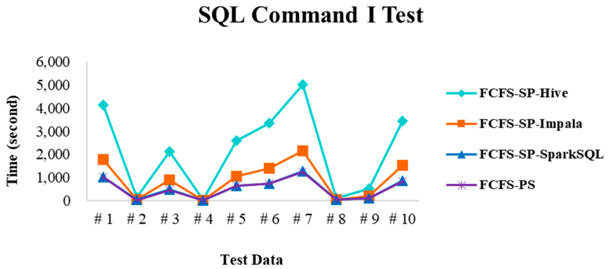
| SQL command I | Only search specific fields |
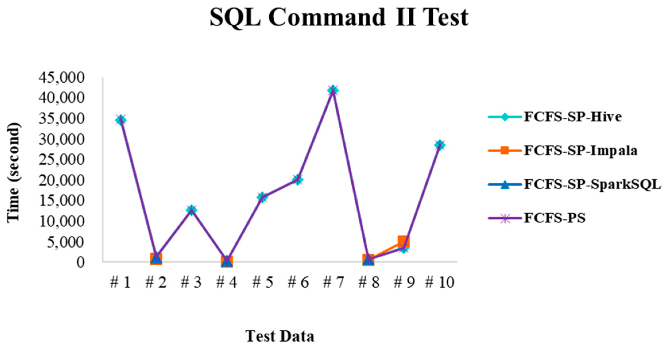
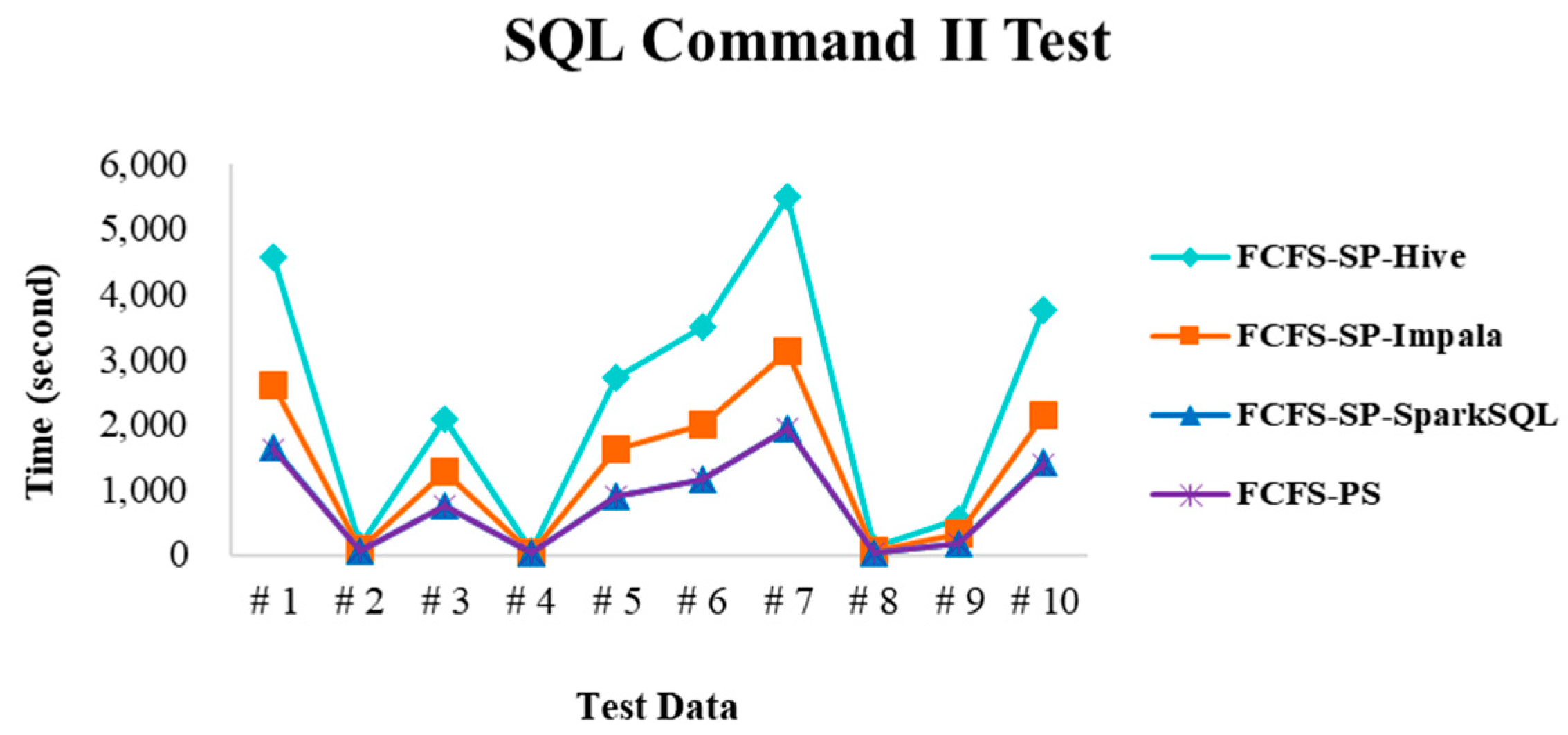
| SQL command II | Search for a particular field and add the comparison condition |
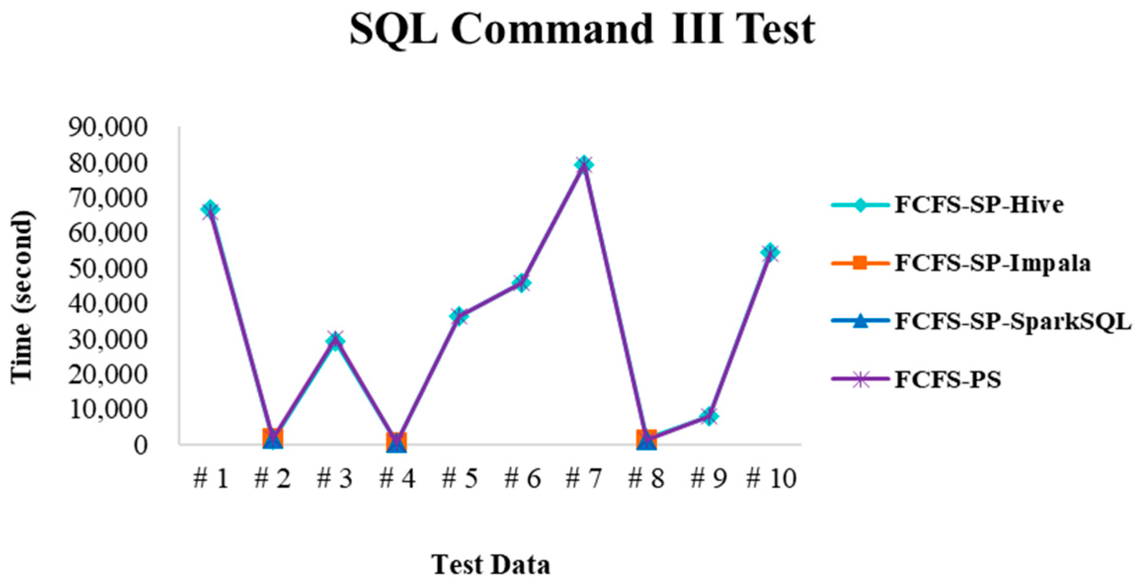
| SQL command III | Execute the commands containing Table JOIN |
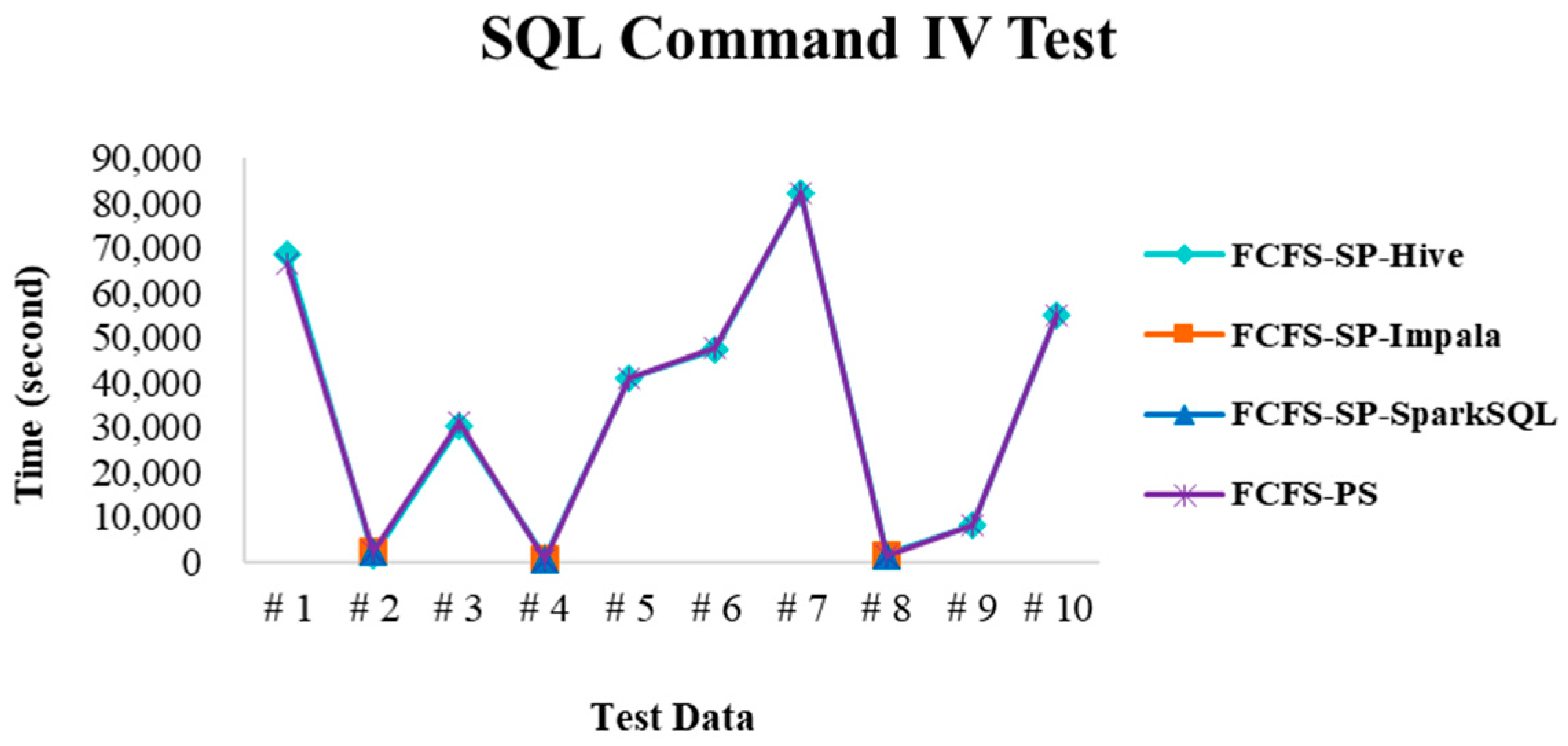
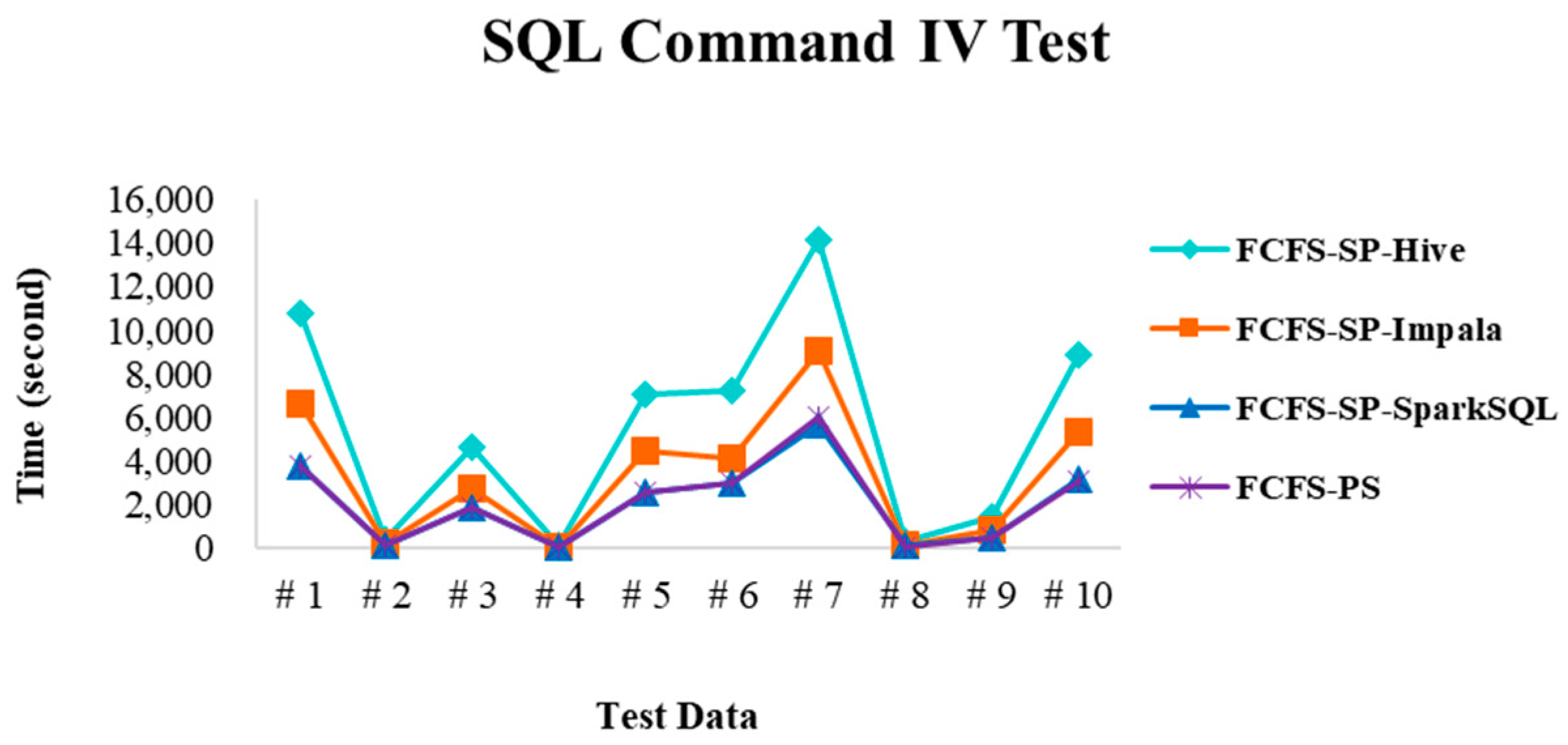
| SQL command IV | Execute the commands containing GROUP BY |
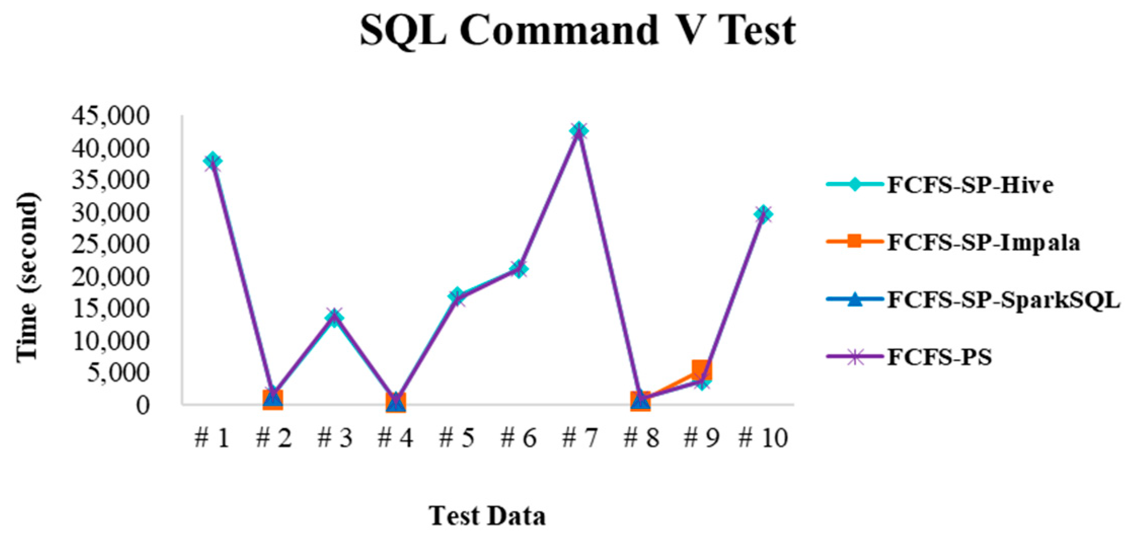
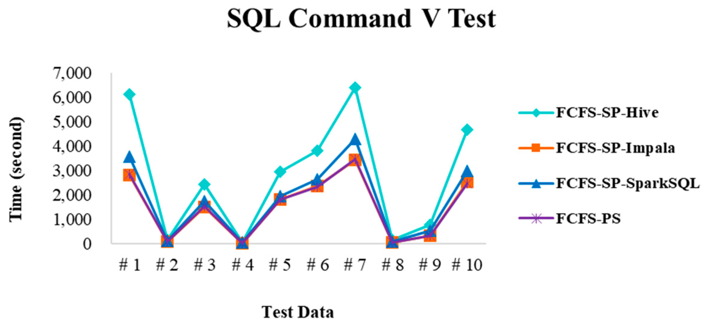
| SQL command V | Execute the commands containing INSERT INTO |
| Tools | Command |
|---|---|
| Hive | Use “enforced hive” command to run the tool |
| Impala | Use “enforced impala” command to run the tool |
| SparkSQL | Use “enforced sparksql” command to run the tool |
| Command | Function |
|---|---|
| sql [sql_cmd] | Enter a SQL query command |
| stat | Displays the current cluster status |
| flush | Clear all in-memory cache |
| purge [days] | Clear part of cache that are not accessed in a number of days |
| display [on|off] | Turn on/off to display search results |
| enforced [name|auto] | Forced to use a specific tool (Hive, Impala, or SparkSQL) |
| Test Environment | Memory Size |
|---|---|
| Test environment I | Reserve 3 GB remaining memory space |
| Test environment II | Reserve 10 GB remaining memory space |
| Test environment III | Allocate all memory space 20 GB |
| No. | Data Size | Codename |
|---|---|---|
| 1 | 850 GB | A |
| 2 | 30 GB | B |
| 3 | 400 GB | C |
| 4 | 10 GB | D |
| 5 | 500 GB | E |
| 6 | 630 GB | F |
| 7 | 1 TB | G |
| 8 | 20 GB | H |
| 9 | 100 GB | I |
| 10 | 700 GB | J |
| Category | Function |
|---|---|
| SQL command I | Only search specific fields e.g., SELECT key FROM test10g ORDER BY val1; |
| SQL command II | Add the comparison condition e.g., SELECT key FROM test10g WHERE val1 + val2 = 250; |
| SQL command III | Execute the commands containing Table JOIN e.g., SELECT test100g.val1, test100g.val2, test10g.val3 FROM test100g, test10g WHERE test100g.val2 = test10g.val2; |
| SQL command IV | Execute the commands containing GROUP BY e.g., SELECT val1, count(val1) FROM test100g GROUP BY val1; |
| SQL command V | Execute the commands containing INSERT INTO e.g., INSERT INTO test10g (key, val1, val2, val3) values (‘key69’, ‘85’, ‘163’, ‘69’); |
| Method | Command |
|---|---|
| Hive | Use “enforced hive” command to run the tool |
| Impala | Use “enforced impala” command to run the tool |
| SparkSQL | Use “enforced sparksql” command to run the tool |
| In-memory Cache | Reaction time when cache hit |
| In-disk Cache | Reaction time when cache hit |
| Method | Environment I | Environment II | Environment III | Weighted Average Execution Time |
|---|---|---|---|---|
| FCFS-SP-Hive | 22,834 | 3604 | 3530 | 3567 |
| FCFS-SP-Impala | - | 2047 | 2033 | 2040 |
| FCFS-SP-SparkSQL | - | 2681 | 1257 | 1969 |
| FCFS-PS | 24,325 | 2169 | 1340 | 1755 |
| Operation | FCFS-SP-Hive | FCFS-SP-Impala | FCFS-SP-SparkSQL | FCFS-PS |
|---|---|---|---|---|
| Environment I | - | - | - | - |
| Environment II | 0.5436 | 0.9940 | 0.7573 | 1.0000 |
| Environment III | 0.3414 | 0.6082 | 0.9934 | 1.0000 |
| Method | Average Normalized PI | Performance Index |
|---|---|---|
| FCFS-SP-Hive | 0.443 | 44 |
| FCFS-SP-Impala | 0.801 | 80 |
| FCFS-SP-SparkSQL | 0.875 | 88 |
| FCFS-PS | 1.000 | 100 |
| No. | Data Size | Use Case | Codename |
|---|---|---|---|
| 1 | 10 GB | World-famous masterpiece | WC |
| 2 | 250 GB | Load of production machine: Overloading | OD |
| 3 | 250 GB | Load of production machine: Underloading | UD |
| 4 | 1 TB | Qualified rate of semiconductor products | YR |
| 5 | 750 GB | Correlation among temperature and people’s power utilization | TE |
| 6 | 750 GB | Correlation among rainfall and people’s power utilization | RE |
| 7 | 100 GB | Flight information in the airport | AP |
| 8 | 500 GB | Traffic violation/accidents | TA |
| Method | Environment I | Environment II | Environment III | Weighted Average Execution Time |
|---|---|---|---|---|
| FCFS-SP-Hive | 33,405 | 5215 | 5045 | 5130 |
| FCFS-SP-Impala | - | 1972 | 2553 | 2262 |
| FCFS-SP-SparkSQL | - | 3647 | 1110 | 2378 |
| FCFS-PS | 33,406 | 2036 | 1105 | 1570 |
| Operation | FCFS-SP-Hive | FCFS-SP-Impala | FCFS-SP-SparkSQL | FCFS-PS |
|---|---|---|---|---|
| Environment I | - | - | - | - |
| Environment II | 0.3781 | 1.0000 | 0.5582 | 1.0000 |
| Environment III | 0.2190 | 0.4329 | 0.9959 | 1.0000 |
| Method | Average Normalized PI | Performance Index |
|---|---|---|
| FCFS-SP-Hive | 0.299 | 30 |
| FCFS-SP-Impala | 0.716 | 72 |
| FCFS-SP-SparkSQL | 0.777 | 78 |
| FCFS-PS | 1.000 | 100 |
© 2018 by the authors. Licensee MDPI, Basel, Switzerland. This article is an open access article distributed under the terms and conditions of the Creative Commons Attribution (CC BY) license (http://creativecommons.org/licenses/by/4.0/).
Share and Cite
Chang, B.R.; Tsai, H.-F.; Lee, Y.-D. Integrated High-Performance Platform for Fast Query Response in Big Data with Hive, Impala, and SparkSQL: A Performance Evaluation. Appl. Sci. 2018, 8, 1514. https://doi.org/10.3390/app8091514
Chang BR, Tsai H-F, Lee Y-D. Integrated High-Performance Platform for Fast Query Response in Big Data with Hive, Impala, and SparkSQL: A Performance Evaluation. Applied Sciences. 2018; 8(9):1514. https://doi.org/10.3390/app8091514
Chicago/Turabian StyleChang, Bao Rong, Hsiu-Fen Tsai, and Yun-Da Lee. 2018. "Integrated High-Performance Platform for Fast Query Response in Big Data with Hive, Impala, and SparkSQL: A Performance Evaluation" Applied Sciences 8, no. 9: 1514. https://doi.org/10.3390/app8091514
APA StyleChang, B. R., Tsai, H.-F., & Lee, Y.-D. (2018). Integrated High-Performance Platform for Fast Query Response in Big Data with Hive, Impala, and SparkSQL: A Performance Evaluation. Applied Sciences, 8(9), 1514. https://doi.org/10.3390/app8091514