Computational Fluid Dynamic Accuracy in Mimicking Changes in Blood Hemodynamics in Patients with Acute Type IIIb Aortic Dissection Treated with TEVAR

 ,
, 

Abstract
:1. Introduction
2. Materials and Methods
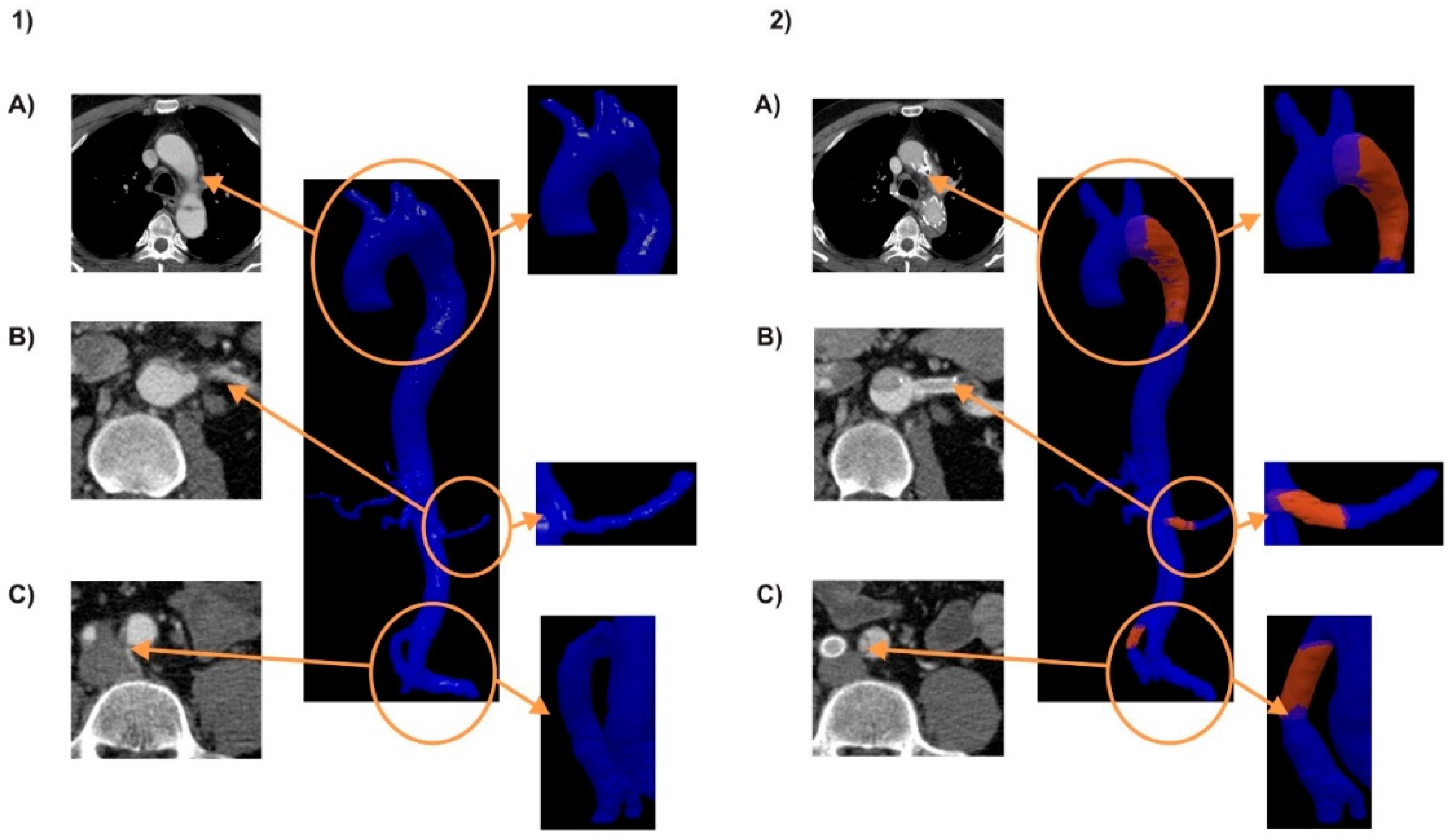
2.1. Materials
2.2. Computational Fluid Dynamics Analysis
2.3. Statistical Analysis
3. Results
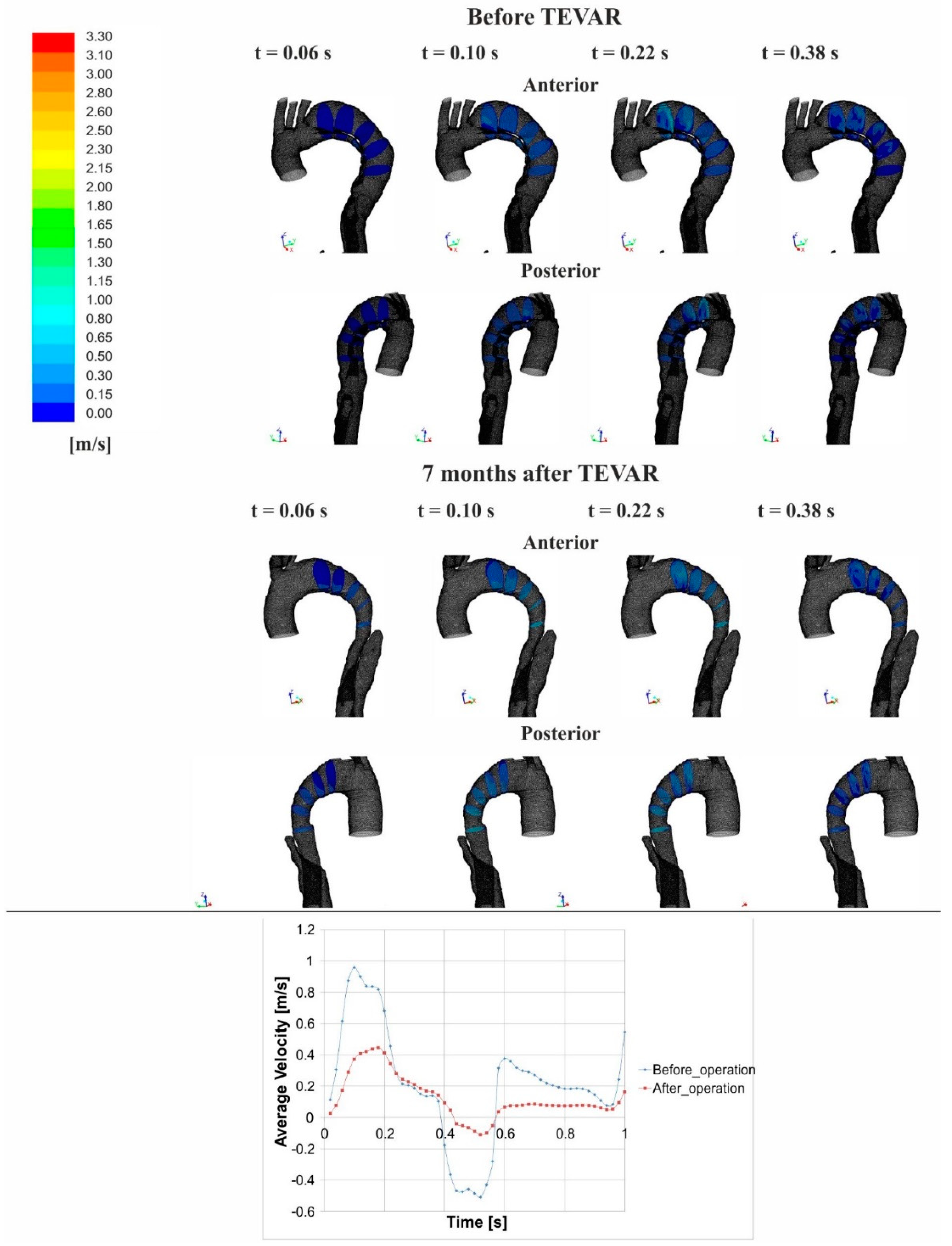
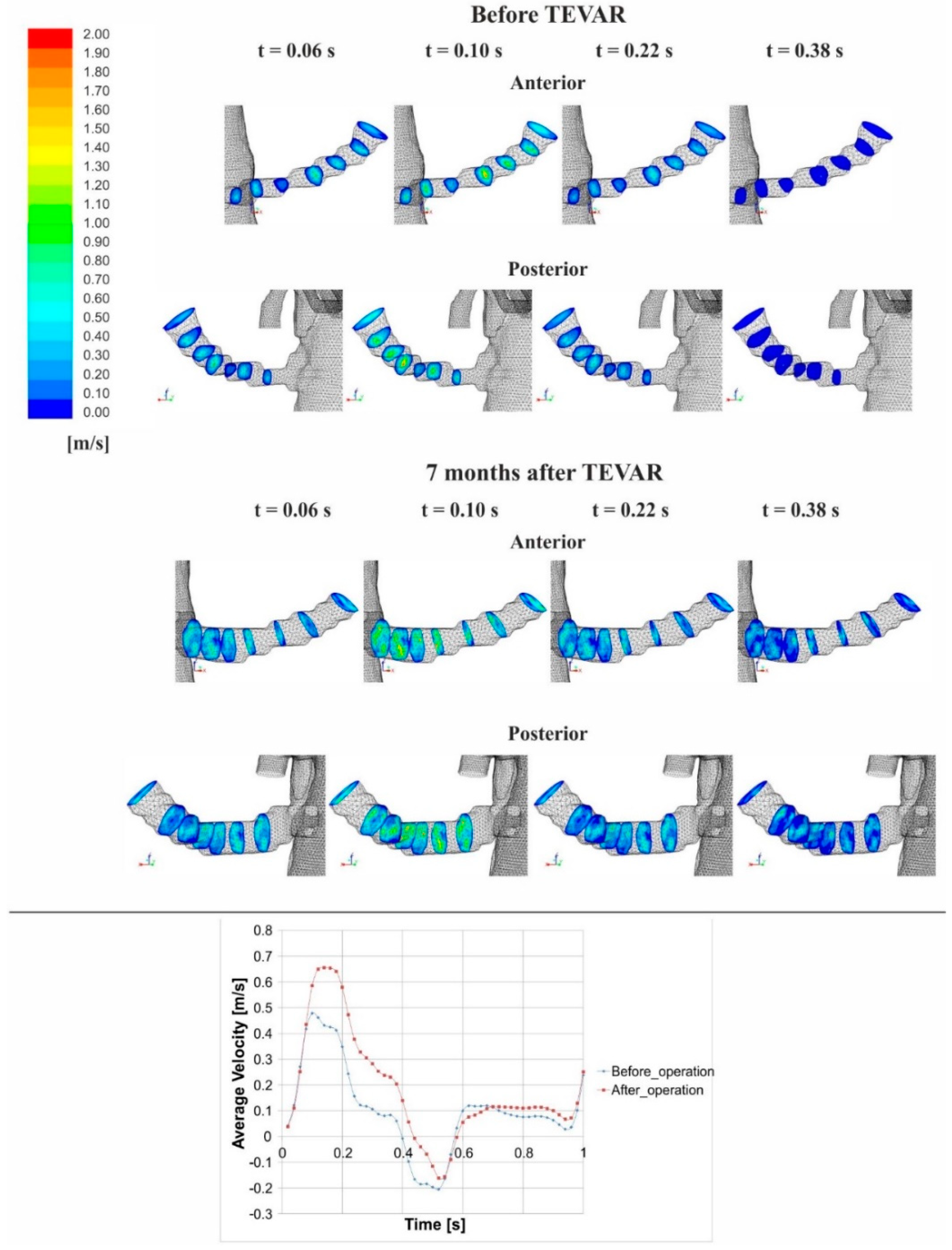
3.1. Flow Analysis
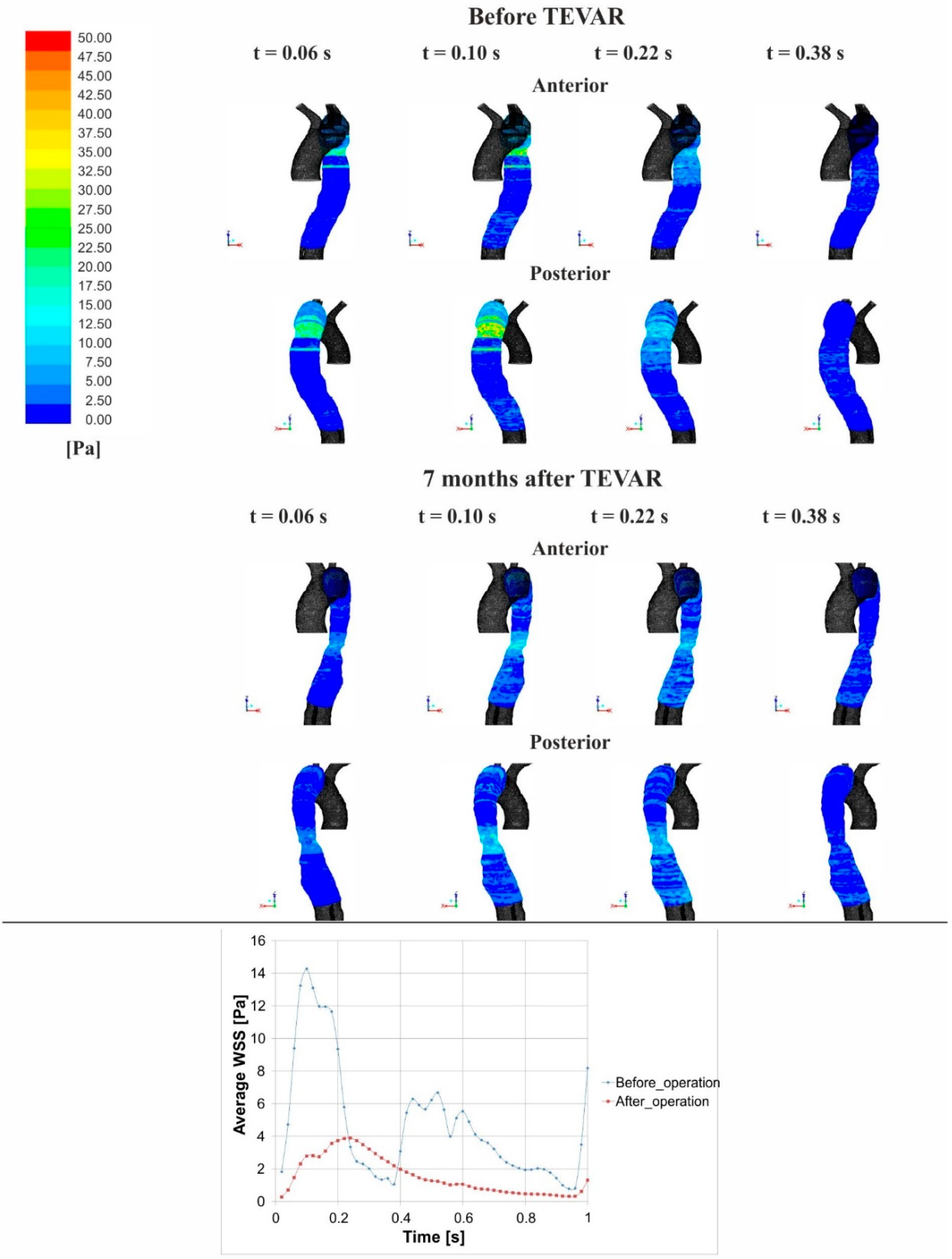
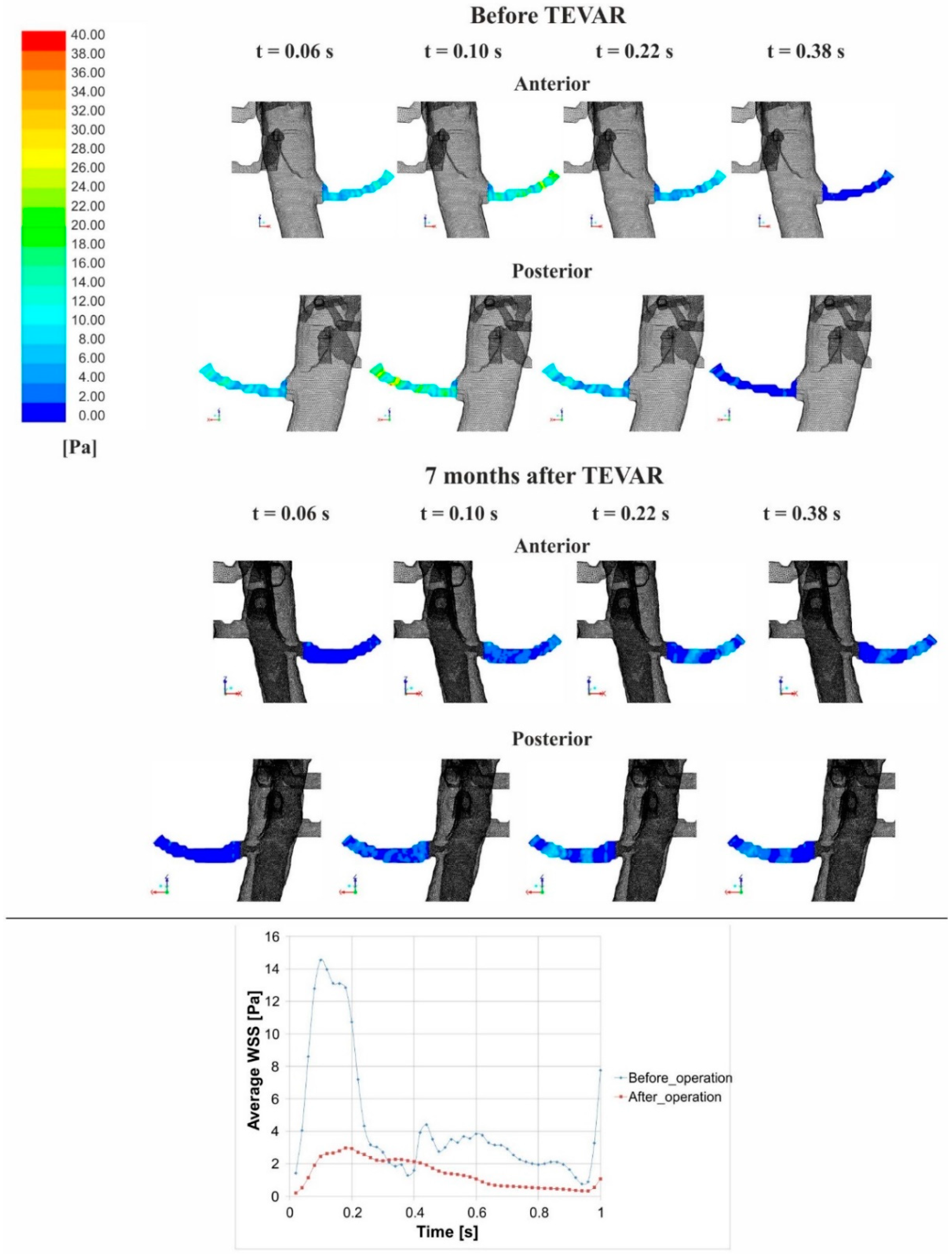
3.2. Stress Analysis
4. Discussion
Limitations to the Study
5. Conclusions
Author Contributions
Funding
Acknowledgments
Conflicts of Interest
References
- Olsson, C.; Thelin, S.; Stahle, E.; Ekbom, A.; Granath, F. Thoracic aortic aneurysm and dissection: Increasing prevalence and improved outcomes reported in a nationwide population-based study of more than 14,000 cases from 1987 to 2002. Circulation 2006, 114, 2611–2618. [Google Scholar] [CrossRef] [PubMed]
- Hagan, P.G.; Nienaber, C.A.; Isselbacher, E.M.; Bruckman, D.; Karavite, D.J.; Russman, P.L.; Evangelista, A.; Fattori, R.; Suzuki, T.; Oh, J.K.; et al. The International Registry of Acute Aortic Dissection (IRAD): New insights into an old disease. JAMA J. Am. Med. Assoc. 2000, 283, 897–903. [Google Scholar] [CrossRef]
- Roberts, C.S.; Roberts, W.C. Aortic dissection with the entrance tear in the descending thoracic aorta. Analysis of 40 necropsy patients. Ann. Surg. 1991, 213, 356–368. [Google Scholar] [CrossRef] [PubMed]
- Suzuki, T.; Mehta, R.H.; Ince, H.; Nagai, R.; Sakomura, Y.; Weber, F.; Sumiyoshi, T.; Bossone, E.; Trimarchi, S.; Cooper, J.V.; et al. Clinical profiles and outcomes of acute type B aortic dissection in the current era: Lessons from the International Registry of Aortic Dissection (IRAD). Circulation 2003, 108 (Suppl. 1), II312–II317. [Google Scholar] [CrossRef] [PubMed]
- Nienaber, C.A.; Fattori, R.; Lund, G.; Dieckmann, C.; Wolf, W.; von Kodolitsch, Y.; Nicolas, V.; Pierangeli, A. Nonsurgical reconstruction of thoracic aortic dissection by stent-graft placement. N. Engl. J. Med. 1999, 340, 1539–1545. [Google Scholar] [CrossRef] [PubMed]
- Dake, M.D.; Kato, N.; Mitchell, R.S.; Semba, C.P.; Razavi, M.K.; Shimono, T.; Hirano, T.; Takeda, K.; Yada, I.; Miller, D.C. Endovascular stent-graft placement for the treatment of acute aortic dissection. N. Engl. J. Med. 1999, 340, 1546–1552. [Google Scholar] [CrossRef] [PubMed]
- Herman, I.M.; Brant, A.M.; Warty, V.S.; Bonaccorso, J.; Klein, E.C.; Kormos, R.L.; Borovetz, H.S. Hemodynamics and the vascular endothelial cytoskeleton. J. Cell Biol. 1987, 105, 291–302. [Google Scholar] [CrossRef] [PubMed] [Green Version]
- Blanco, P.J.; Pivello, M.R.; Urquiza, S.A.; Feijoo, R.A. On the potentialities of 3D-1D coupled models in hemodynamics simulations. J. Biomech. 2009, 42, 919–930. [Google Scholar] [CrossRef] [PubMed]
- Polanczyk, A.; Podgorski, M.; Wozniak, T.; Stefanczyk, L.; Strzelecki, M. Computational Fluid Dynamics as an Engineering Tool for the Reconstruction of Hemodynamics after Carotid Artery Stenosis Operation: A Case Study. Medicina 2018, 54, 42. [Google Scholar] [CrossRef]
- Cheng, Z.; Tan, F.P.; Riga, C.V.; Bicknell, C.D.; Hamady, M.S.; Gibbs, R.G.; Wood, N.B.; Xu, X.Y. Analysis of flow patterns in a patient-specific aortic dissection model. J. Biomech. Eng. 2010, 132, 051007. [Google Scholar] [CrossRef] [PubMed]
- Polanczyk, A.; Strzelecki, M.; Wozniak, T.; Szubert, W.; Stefanczyk, L. 3D Blood Vessels Reconstruction Based on Segmented CT Data for Further Simulations of Hemodynamic in Human Artery Branches. Found. Comput. Decis. Sci. 2017, 42, 359–371. [Google Scholar] [CrossRef] [Green Version]
- Shahcheraghi, N.; Dwyer, H.A.; Cheer, A.Y.; Barakat, A.I.; Rutaganira, T. Unsteady and three-dimensional simulation of blood flow in the human aortic arch. J. Biomech. Eng. 2002, 124, 378–387. [Google Scholar] [CrossRef] [PubMed]
- Lam, S.K.; Fung, G.S.; Cheng, S.W.; Chow, K.W. A computational study on the biomechanical factors related to stent-graft models in the thoracic aorta. Med. Biol. Eng. Comput. 2008, 46, 1129–1138. [Google Scholar] [CrossRef] [PubMed]
- Tse, K.M.; Chiu, P.; Lee, H.P.; Ho, P. Investigation of hemodynamics in the development of dissecting aneurysm within patient-specific dissecting aneurismal aortas using computational fluid dynamics (CFD) simulations. J. Biomech. 2011, 44, 827–836. [Google Scholar] [CrossRef] [PubMed]
- Kizilova, N. Computational approach to optimal transport network construction in biomechanics. Lect. Notes Comput. Sci. 2004, 3044, 476–485. [Google Scholar]
- Amblard, A.; Berre, H.W.L.; Bou-Said, B.; Brunet, M. Analysis of type I endoleaks in a stented abdominal aortic aneurysm. Med. Eng. Phys. 2009, 31, 27–33. [Google Scholar] [CrossRef] [PubMed]
- Xenos, M.; Rambhia, S.H.; Alemu, Y.; Einav, S.; Labropoulos, N.; Tassiopoulos, A.; Ricotta, J.J.; Bluestein, D. Patient-Based Abdominal Aortic Aneurysm Rupture Risk Prediction with Fluid Structure Interaction Modeling. Ann. Biomed. Eng. 2010, 38, 3323–3337. [Google Scholar] [CrossRef] [PubMed] [Green Version]
- Auer, M.; Gasser, T.C. Reconstruction and finite element mesh generation of abdominal aortic aneurysms from computerized tomography angiography data with minimal user interactions. IEEE Trans. Med. Imaging 2010, 29, 1022–1028. [Google Scholar] [CrossRef] [PubMed]
- Polanczyk, A.; Klinger, M.; Nanobachvili, J.; Huk, I.; Neumayer, C. Artificial Circulatory Model for Analysis of Human and Artificial Vessels. Appl. Sci. 2018, 8, 1017. [Google Scholar] [CrossRef]
- Papathanasopoulou, P.; Zhao, S.; Kohler, U.; Robertson, M.B.; Long, Q.; Hoskins, P.; Xu, X.Y.; Marshall, I. MRI measurement of time-resolved wall shear stress vectors in a carotid bifurcation model, and comparison with CFD predictions. J. Magn. Reson. Imaging JMRI 2003, 17, 153–162. [Google Scholar] [CrossRef] [PubMed] [Green Version]
- Fillinger, M.F.; Greenberg, R.K.; McKinsey, J.F.; Chaikof, E.L.; Society for Vascular Surgery Ad Hoc Committee on TRS. Reporting standards for thoracic endovascular aortic repair (TEVAR). J. Vasc. Surg. 2010, 52, 1022–1033. [Google Scholar] [CrossRef] [PubMed]
- Polanczyk, A.; Podyma, M.; Trebinski, L.; Chrzastek, J.; Zbicinski, I.; Stefanczyk, L. A Novel Attempt to Standardize Results of CFD Simulations Basing on Spatial Configuration of Aortic Stent-Grafts. PLoS ONE 2016, 11, e0153332. [Google Scholar] [CrossRef] [PubMed]
- Polanczyk, A.; Wozniak, T.; Strzelecki, M.; Szubert, W.; Stefanczyk, L. Evaluating an algorithm for 3D reconstruction of blood vessels for further simulations of hemodynamic in human artery branches. IEEE Xplore Dig. Libr. 2016, 5, 103–107. [Google Scholar]
- Polańczyk, A.; Podyma, M.; Stefańczyk, L.; Zbiciński, I. Effects of stent-graft geometry and blood hematocrit on hemodynamic in Abdominal Aortic Aneurysm. Chem. Process Eng. 2012, 33, 53–62. [Google Scholar] [CrossRef]
- Polanczyk, A.; Piechota-Polanczyk, A.; Stefanczyk, L. A new approach for the pre-clinical optimization of a spatial configuration of bifurcated endovascular prosthesis placed in abdominal aortic aneurysms. PLoS ONE 2017, 12, e0182717. [Google Scholar] [CrossRef] [PubMed]
- Hoskins, P.R. Simulation and validation of arterial ultrasound imaging and blood flow. Ultrasound Med. Biol. 2008, 34, 693–717. [Google Scholar] [CrossRef] [PubMed]
- Polanczyk, A.; Podyma, M.; Stefanczyk, L.; Szubert, W.; Zbicinski, I. A 3D model of thrombus formation in a stent-graft after implantation in the abdominal aorta. J. Biomech. 2015, 48, 425–431. [Google Scholar] [CrossRef] [PubMed]
- Granata, A.; Fiorini, F.; Andrulli, S.; Logias, F.; Gallieni, M.; Romano, G.; Sicurezza, E.; Fiore, C.E. Doppler ultrasound and renal artery stenosis: An overview. J. Ultrasound 2009, 12, 133–143. [Google Scholar] [CrossRef] [PubMed] [Green Version]
- Cheng, Z.; Juli, C.; Wood, N.B.; Gibbs, R.G.; Xu, X.Y. Predicting flow in aortic dissection: Comparison of computational model with PC-MRI velocity measurements. Med. Eng. Phys. 2014, 36, 1176–1184. [Google Scholar] [CrossRef] [PubMed]
- Dillon-Murphy, D.; Noorani, A.; Nordsletten, D.; Figueroa, C.A. Multi-modality image-based computational analysis of haemodynamics in aortic dissection. Biomech. Model. Mechanobiol. 2016, 15, 857–876. [Google Scholar] [CrossRef] [PubMed]
- Yu, S.C.; Liu, W.; Wong, R.H.; Underwood, M.; Wang, D. The Potential of Computational Fluid Dynamics Simulation on Serial Monitoring of Hemodynamic Change in Type, B. Aortic Dissection. Cardiovasc. Interv. Radiol. 2016, 39, 1090–1098. [Google Scholar] [CrossRef] [PubMed]
- Hoshina, K.; Sho, E.; Sho, M.; Nakahashi, T.K.; Dalman, R.L. Wall shear stress and strain modulate experimental aneurysm cellularity. J. Vasc. Surg. 2003, 37, 1067–1074. [Google Scholar] [CrossRef]
- Rudenick, P.A.; Bijnens, B.H.; Garcia-Dorado, D.; Evangelista, A. An in vitro phantom study on the influence of tear size and configuration on the hemodynamics of the lumina in chronic type B. aortic dissections. J. Vasc. Surg. 2013, 57, 464–474. [Google Scholar] [CrossRef] [PubMed]
- Ben Ahmed, S.; Dillon-Murphy, D.; Figueroa, C.A. Computational Study of Anatomical Risk Factors in Idealized Models of Type, B. Aortic Dissection. Eur. J. Vasc. Endovasc. Surg. Off. J. Eur. Soc. Vasc. Surg. 2016, 52, 736–745. [Google Scholar] [CrossRef] [PubMed]
- Karmonik, C.; Partovi, S.; Muller-Eschner, M.; Bismuth, J.; Davies, M.G.; Shah, D.J.; Loebe, M.; Böckler, D.; Lumsden, A.B.; von Tengg-Kobligk, H. Longitudinal computational fluid dynamics study of aneurysmal dilatation in a chronic DeBakey type III aortic dissection. J. Vasc. Surg. 2012, 56, 260–263. [Google Scholar] [CrossRef] [PubMed]
- Georgakarakos, E.; Ioannou, C.V.; Kamarianakis, Y.; Papaharilaou, Y.; Kostas, T.; Manousaki, E.; Katsamouris, A.N. The role of geometric parameters in the prediction of abdominal aortic aneurysm wall stress. Eur. J. Vasc. Endovasc. Surg. Off. J. Eur. Soc. Vasc. Surg. 2010, 39, 42–48. [Google Scholar] [CrossRef] [PubMed]
- Doyle, B.J.; Callanan, A.; Burke, P.E.; Grace, P.A.; Walsh, M.T.; Vorp, D.A.; McGloughlin, T.M. Vessel asymmetry as an additional diagnostic tool in the assessment of abdominal aortic aneurysms. J. Vasc. Surg. 2009, 49, 443–454. [Google Scholar] [CrossRef] [PubMed] [Green Version]
- Duvernois, V.; Marsden, A.L.; Shadden, S.C. Lagrangian analysis of hemodynamics data from FSI simulation. Int. J. Numer. Methods Biomed. Eng. 2013, 29, 445–461. [Google Scholar] [CrossRef] [PubMed]
- Xiang, J.; Tremmel, M.; Kolega, J.; Levy, E.I.; Natarajan, S.K.; Meng, H. Newtonian viscosity model could overestimate wall shear stress in intracranial aneurysm domes and underestimate rupture risk. J. Neurointerv. Surg. 2012, 4, 351–357. [Google Scholar] [CrossRef] [PubMed]


| Name | Patient 1 | Patient 2 | Patient 3 | Patient 4 | Patient 5 |
|---|---|---|---|---|---|
| Dissection Type | IIIb | IIIb | IIIb | IIIb | IIIb |
| Entry Tear | Proximal to the left subclavian artery (LSA) (zone number 4 according to Fillinger et al., 2010) | ||||
| End of Dissection | Right iliac artery (zone number 9 according to Fillinger et al., 2010) | Right iliac artery (zone number 9 according to Fillinger et al., 2010) | Right iliac artery (zone number 9 according to Fillinger et al., 2010) | Left renal artery (zone number 8 according to Fillinger et al., 2010) | Left renal artery (zone number 8 according to Fillinger et al., 2010) |
| Vascular Prosthesis | One stent-graft (115 mm) (zone number 3–4 according to Fillinger et al., 2010), two self-expanded stents (left renal artery (zone number 10 according to Fillinger et al., 2010) and right iliac artery (zone number 8 according to Fillinger et al., 2010)) (25 mm renal, 25 mm iliac) | One stent-graft (117 mm) (zone number 3–4 according to Fillinger et al., 2010), two self-expanded stents (left renal artery (zone number 10 according to Fillinger et al., 2010) and right iliac artery (zone number 8 according to Fillinger et al., 2010)) (30 mm renal, 25 mm iliac) | One stent-graft (118 mm) (zone number 3–4 according to Fillinger et al., 2010), two self-expanded stents (left renal artery (zone number 10 according to Fillinger et al., 2010) and right iliac artery (zone number 8 according to Fillinger et al., 2010)) (25 mm renal, 30 mm iliac) | One stent-graft (120 mm) (zone number 3–4 according to Fillinger et al., 2010), one self-expanded stent (right iliac artery (zone number 8 according to Fillinger et al., 2010)) (27 mm renal) | One stent-graft (120 mm) (zone number 3–4 according to Fillinger et al., 2010), one self-expanded stent (right iliac artery (zone number 8 according to Fillinger et al., 2010)) (30 mm renal) |
| Artery Type | Blood Flow [mL/s] | |||||
|---|---|---|---|---|---|---|
| USG-Doppler | CFD | |||||
| Pre-TEVAR Median [Q1;Q2] | Post TEVAR Median [Q1;Q2] | p Value | Pre TEVAR Median [Q1;Q2] | Post TEVAR Median [Q1;Q2] | p Value | |
| Thoracic trunk | 7.724 (7.089; 9.600) | 65.220 (64.990; 65.300) | p = 0.043 | 9.100 (9.100;9.100) | 61.720 (61.700;63.050) | p = 0.043 |
| Brachiocephalic trunk | 5.300 (4.810;5.920) | 5.050 (4.370;5.200) | p = 0.043 | 5.470 (4.760;5.848) | 4.860 (4.760;5.280) | p = 0.273 |
| Carotid arteries | 4.840 (4.500;5.360) | 4.610 (4.230;5.100) | p = 0.043 | 5.030 (4.470;5.320) | 4.620 (4.470;5.070) | p = 0.715 |
| Subclavian arteries | 4.290 (4.140;4.720) | 4.170 (4.020;4.400) | p = 0.043 | 4.250 (4.010;4.664) | 4.110 (3.820;4.250) | p = 0.273 |
| Renal arteries | 9.300 (8.870;9.430) | 9.705 (9.500;9.925) | p = 0.043 | 9.280 (9.175;9.472) | 10.400 (9.885;10.495) | p = 0.043 |
| Iliac arteries | 2.320 (2.135;2.377) | 1.985 (1.912;2.050) | p = 0.079 | 2.135 (2.045;2.135) | 2.007 (1.947;2.047) | p = 0.079 |
| Artery Type | Blood Velocity [m/s] | |||||
|---|---|---|---|---|---|---|
| USG-Doppler | CFD | |||||
| Pre TEVAR Median [Q1;Q2] | Post TEVAR Median [Q1;Q2] | p Value | Pre TEVAR Median [Q1;Q2] | Post TEVAR Median [Q1;Q2] | p Value | |
| Thoracic trunk | 0.273 (0.250;0.339) | 0.223 (0.208;0.255) | p = 0.043 | 0.321 (0.321;0.321) | 0.217 (0.203;0.239) | p = 0.043 |
| Renal arteries | 0.315 (0.306;0.328) | 0.343 (0.335;0.351) | p = 0.043 | 0.324 (0.317;0.328) | 0.355 (0.349;0.371) | p = 0.043 |
| Iliac arteries | 0.034 (0.034;0.035) | 0.032 (0.031;0.034) | p = 0.079 | 0.033 (0.032;0.035) | 0.031 (0.031;0.031) | p = 0.079 |
© 2018 by the authors. Licensee MDPI, Basel, Switzerland. This article is an open access article distributed under the terms and conditions of the Creative Commons Attribution (CC BY) license (http://creativecommons.org/licenses/by/4.0/).
Share and Cite
Polanczyk, A.; Piechota-Polanczyk, A.; Domenig, C.; Nanobachvili, J.; Huk, I.; Neumayer, C. Computational Fluid Dynamic Accuracy in Mimicking Changes in Blood Hemodynamics in Patients with Acute Type IIIb Aortic Dissection Treated with TEVAR. Appl. Sci. 2018, 8, 1309. https://doi.org/10.3390/app8081309
Polanczyk A, Piechota-Polanczyk A, Domenig C, Nanobachvili J, Huk I, Neumayer C. Computational Fluid Dynamic Accuracy in Mimicking Changes in Blood Hemodynamics in Patients with Acute Type IIIb Aortic Dissection Treated with TEVAR. Applied Sciences. 2018; 8(8):1309. https://doi.org/10.3390/app8081309
Chicago/Turabian StylePolanczyk, Andrzej, Aleksandra Piechota-Polanczyk, Christoph Domenig, Josif Nanobachvili, Ihor Huk, and Christoph Neumayer. 2018. "Computational Fluid Dynamic Accuracy in Mimicking Changes in Blood Hemodynamics in Patients with Acute Type IIIb Aortic Dissection Treated with TEVAR" Applied Sciences 8, no. 8: 1309. https://doi.org/10.3390/app8081309