1. Introduction
Biomass and especially woodchips is fuel with very unstable composition (varying moisture content in wood, type and quality of wood) in comparison with fossil fuels (natural gas, oil), and considering its heterogeneous characteristics it is necessary to control the amount of combustion air during fuel supply into the boiler furnace and also during the combustion phase [
1,
2]. If the amount of air is less than optimal, incomplete combustion occurs and the flue gas contains combustible components. On the other hand, in the case of supplying a large amount of combustion air, an energy loss (called flue loss) occurs. There is also a necessity to divide the supplied combustion air into primary air and secondary air [
2,
3]. Besides that, it is necessary to provide a high enough combustion temperature and time to complete the biomass combustion process. So there is a need to achieve simultaneously controlled values of the required boiler heat output and optimal conditions for the combustion process from both the efficiency and emissions point of view [
4,
5,
6]. Therefore, the operation of biomass-fired boilers has to be properly controlled using a classical cascade [
7] and also advanced control algorithms and methods [
8,
9] with the possibility of on-line system monitoring [
10].
In medium-scale biomass-fired boilers, the amount of combustion air is in standard circumstances controlled by means of a Lambda probe that measures oxygen (O
2) concentration in a flue gas. In order to increase combustion efficiency and simultaneously to increase the amount of heat produced and to decrease harmful emissions, new control algorithms were designed based on information not only about O
2 concentration in the flue gas but also about the trend of carbon monoxide (CO) emissions. These algorithms were implemented into the control systems of the biomass-fired boiler with the aim of reaching complete combustion with minimum excess of combustion air. It was proven that a low-cost wide band Lambda probe and simple CO sensor can be used for cost-effective biomass combustion control in medium-scale and, after some simplification, also in small-scale biomass-fired boilers [
11,
12,
13]. However, due to strong interference in one type of boiler, the task of how to define a trend function of measured variables (especially CO emissions and O
2 concentration in flue gas) had to be solved. Another problem that arose was how to correctly use the noisy measured data for biomass combustion control because it was difficult to apply in a process control system [
14]. The measured values were influenced by various transfer errors, disturbances and external interferences and for that reason the measured data had to be appropriately smoothed and filtered.
There are many types of digital filters that can be used for signal filtration [
15,
16]. One of the interesting examples of digital filters is the infinite impulse response (IIR) filter. This filter consists of feedforward and feedback and it is also called the auto regressive moving average (ARMA) filter. A special group of digital filters is a group of finite impulse response (FIR) filters, also called moving average (MA) filters [
17,
18,
19]. A filter that exhibits the properties of superposition, homogeneity, and shift invariance is called a linear time invariant (LTI) filter [
20]. Its advantage is that one-dimensional LTI systems can be described by linear differential equations with constant coefficients.
Some of filters mentioned above are not convenient for biomass combustion signal filtering, because stochastic elements have an influence on the output of the filter (recursive IIR filters). For example, MA filters with exponential forgetting are not useful due to the algorithm of weight-counting [
21]. The others are useful only with a mathematical model of the system (e.g., Kalman filter) [
22].
2. Membership Function Filter
2.1. Demands on the Filter
Firstly, it must be emphasized that the supposed values of measured variables are predetermined (they are in known intervals) and it is necessary to appropriately eliminate extremely different values which arise from random interference during signal transmission. In the case of a long-lasting trend of measured values out of a supposed interval (for example, considerable increasing or decreasing of a measured variable) values are not eliminated. So the basic demand on the filter is that random changes would not have an effect on the filter output and, therefore, on controlled variables. Long-lasting changes out of the supposed interval must have an influence on the filter output and must be signified on the trend of measured variables.
Further reasons for the design of the specific filter are:
- (1)
Considering a filter application in digital controllers with limited computing capacity, the algorithm of the proposed filter has to be simple mathematically and relatively easily programmable.
- (2)
Using classical approximation methods by linear or non-linear trend functions is problematic, considering the huge number of random values in measured function behaviors as a result of strong interferences.
- (3)
Using typical known filters (for example the Kalman filter) is questionable, considering that mathematical description of the measured variables behavior is unknown.
For these reasons, a filtering method using a weighted moving average was chosen with weight calculation on the basis of different membership functions.
2.2. Description of the Filtering Method
The membership function filter, as it was named, is similar to the weight moving average filter, which is counted from k measured values, but weights are calculated based on the membership function for belonging to a set of k measured values. This is the most important difference from a weighted moving average filter, because if a set of measured values has changed, weights also change due to their dependence on an average set of values. Mathematically, such a filter can be expressed as follows.
The sample of the non-filtered signal
includes deterministic
and stochastic
elements:
The stochastic part of the signal can be suppressed by the substitution for the counted moving weight average from the last
k samples of the non-filtered signal:
where
j = 1, …,
k and
k is the chosen number of samples,
are last
k signal samples which contain the deterministic and stochastic element, and
wj are counted weights from interval (0–1〉 for
k last obtained signal samples.
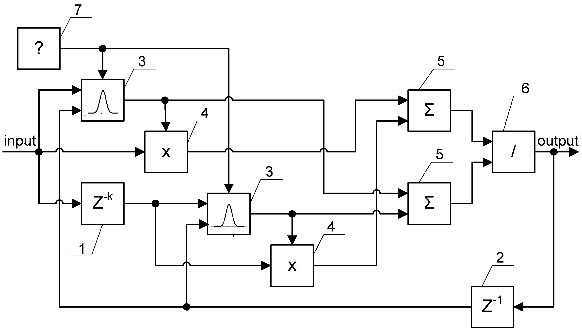
The principle diagram of such a membership function filter for
k samples of the non-filtered signal is in
Figure 1. It consists of block 1 for sampling of the non-filtered signal, block 2 for sampling of the filtered signal, blocks 3 for weight assignment of non-filtered samples according to selected membership function by block 7, and blocks 4 (multiplication), 5 (summation) and 6 (division) for calculation of the filter output according to Equation (2). The input to the filter is the current sample of the non-filtered signal containing deterministic and stochastic parts. For this sample and also for previous
k − 1 stored samples, weights are calculated according to selected membership function and multiplied by used samples. In the next step, the sum of products and the sum of weights are calculated in order to be divided, and the new filtered sample is obtained from the filter output. Finally, the output of the filter is saved for weight counting in time
ti+1. Due to division in the output block of the filter, there is a condition for filter implementation that the sum of weights can be never equal to zero.
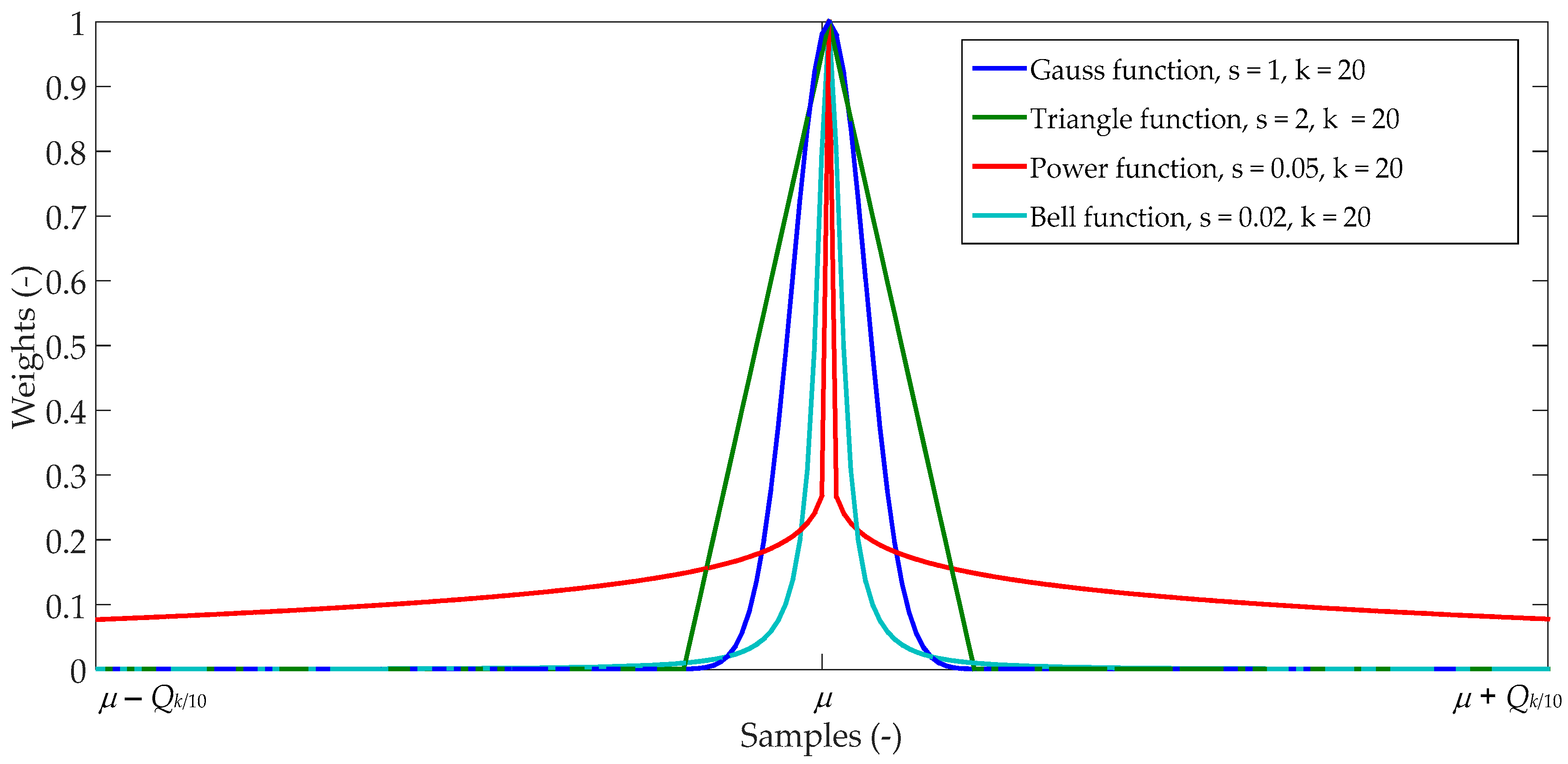
2.3. Membership Function and Its Weights Calculus
The membership function of several different distribution functions can be chosen as shown in
Figure 2. For a normal distribution function (Gauss function), the Equation is:
After some simplifications this can be derived for weight calculation:
where
s is defined as sensitivity and
μ is last weighted average.
Similarly, for the Triangle function:
Power function:
and Bell function:
2.4. Filter Parameters
Operation of the membership function filter depends mainly on two parameters: sensitivity
s of the membership function and the number of samples
k stored in the filter. In
Figure 3,
Figure 4,
Figure 5 and
Figure 6, a comparison of various sensitivity
s is shown for different membership functions with weight calculations according to Equations (4)–(7).
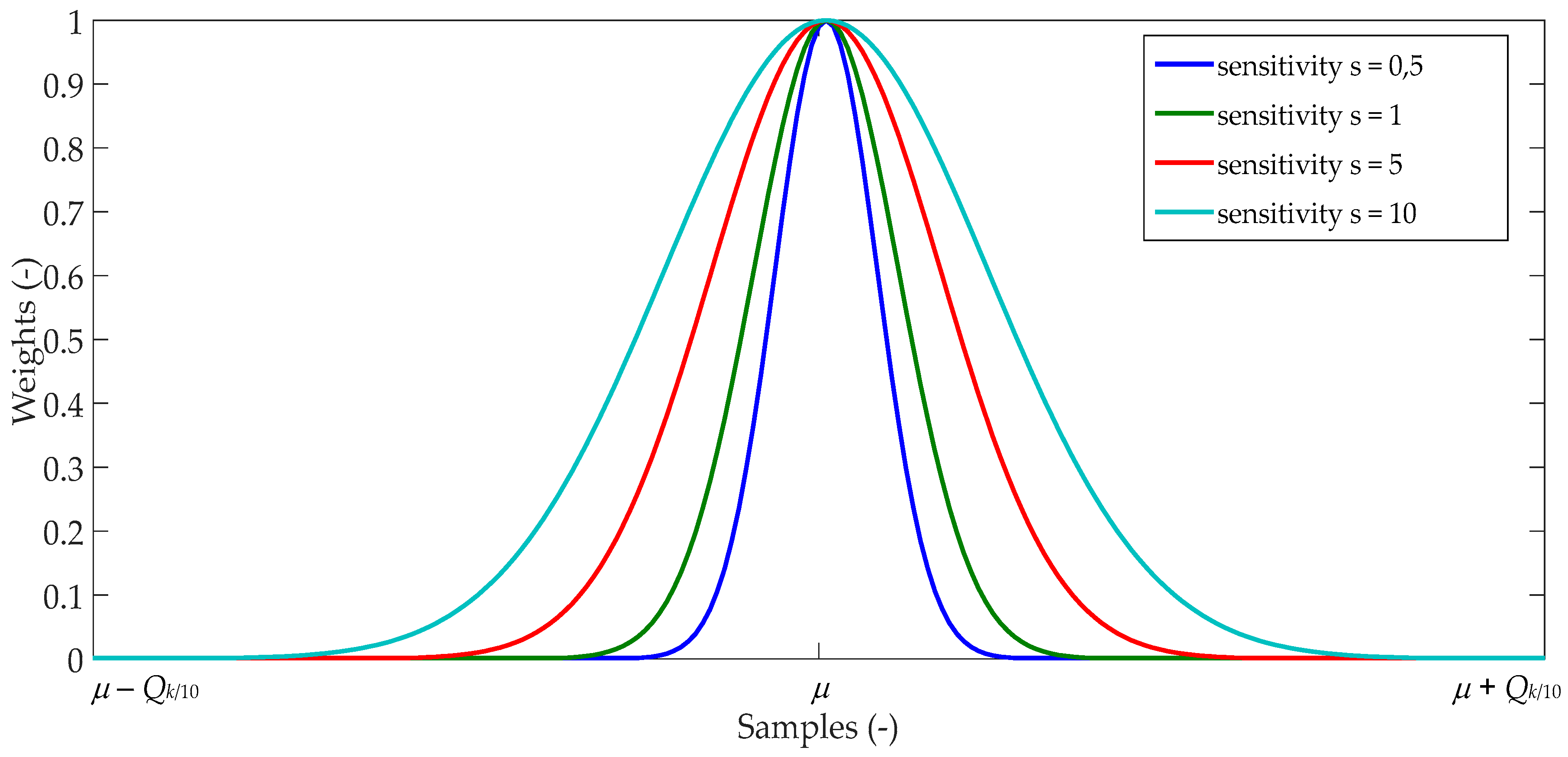
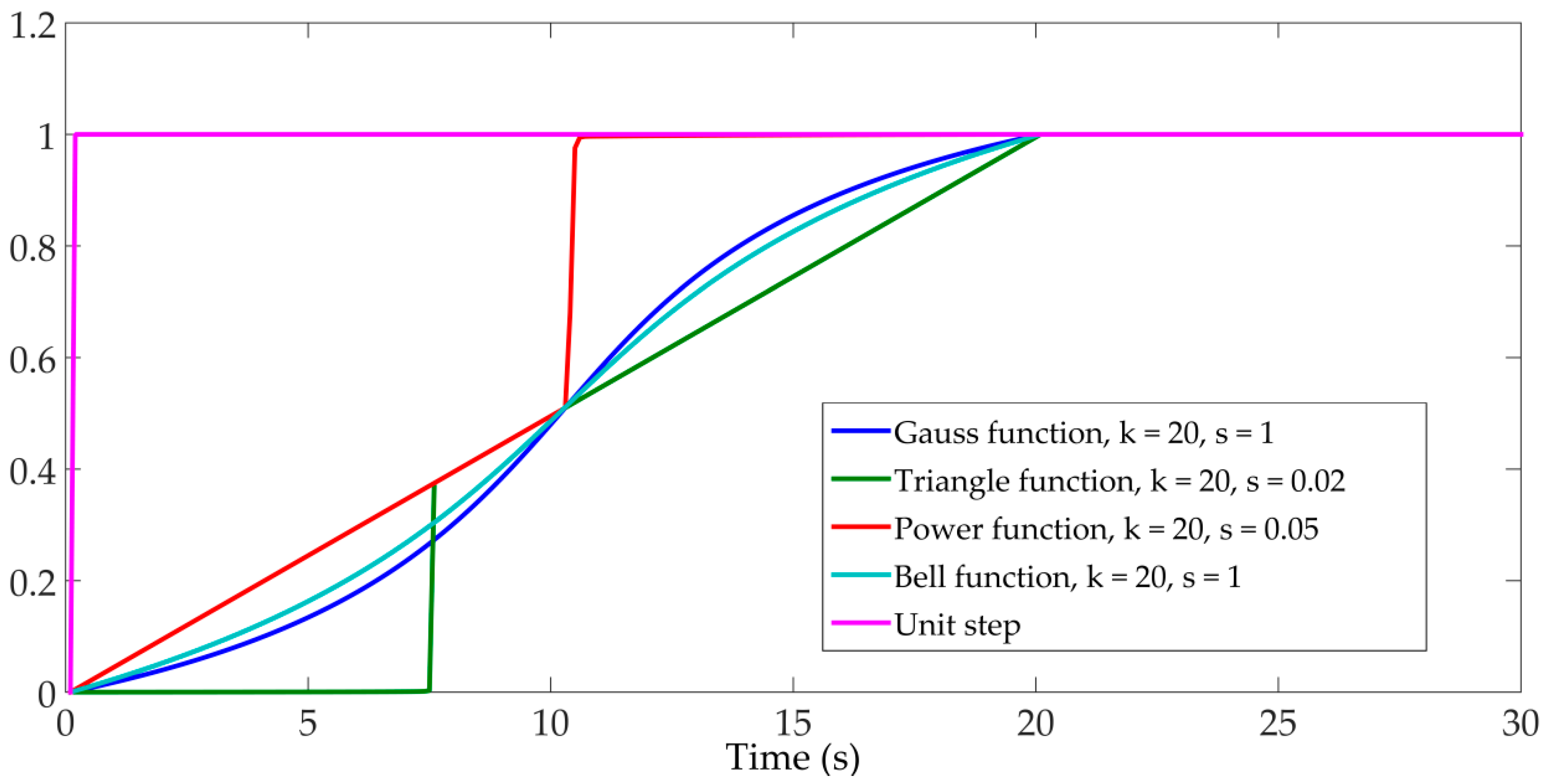
In
Figure 3, there are weights calculated according to Gauss function. Referring to
Figure 3, by filtering using Equation (4), samples which are closer to average
μ have an assignment of higher weights and only samples further away from the average
μ have an assignment of very low weight. If the sensitivity coefficient
s is lower, the interval of higher weights will be narrower, i.e. only samples which are very near to average
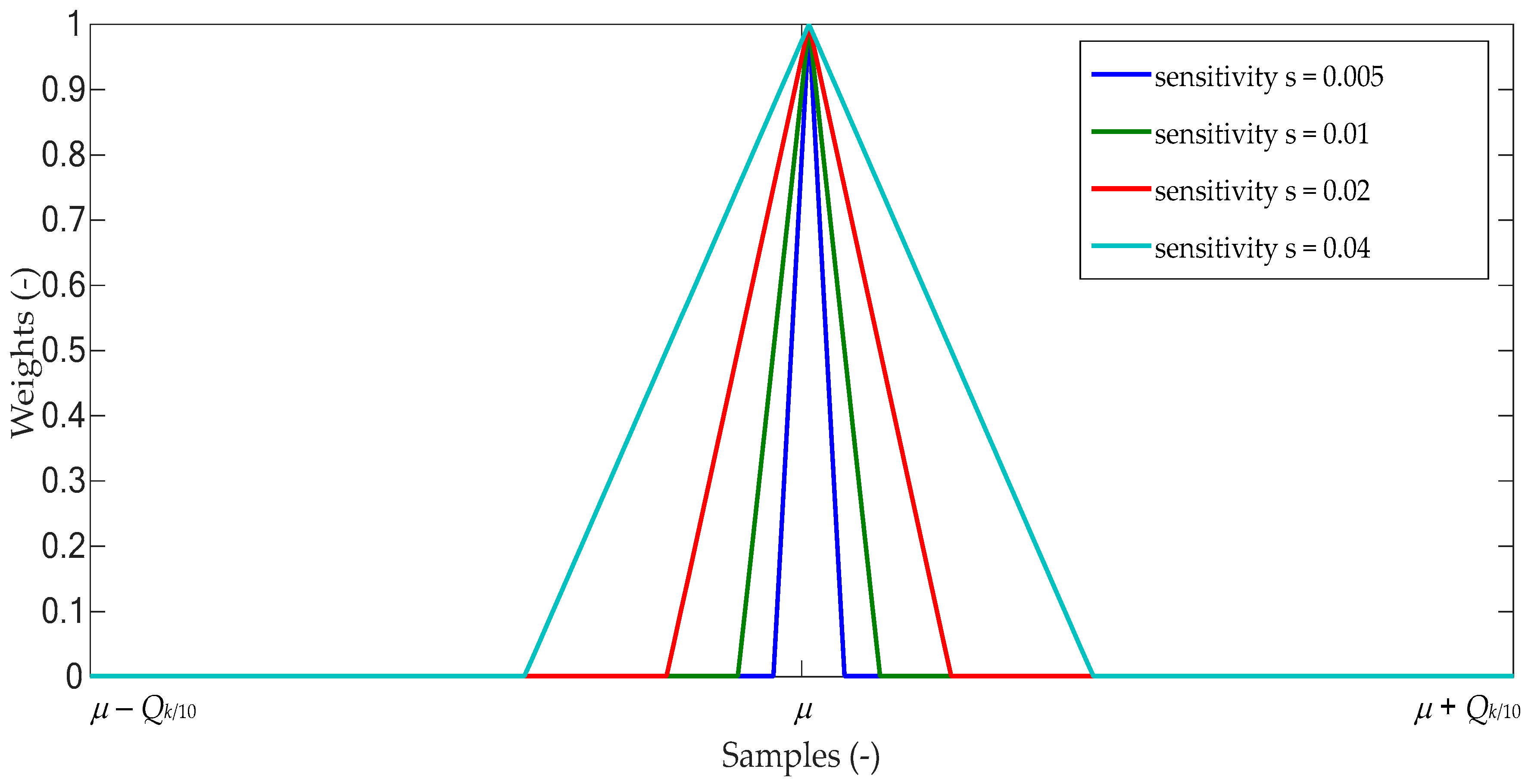
μ have an assignment of high weights. The Triangle function in Equation (5) is also suitable for using as a membership function, because as can be seen in
Figure 4 it has a similar results of weights assignment as the Gauss or Bell functions, but does not have a concave shape near average
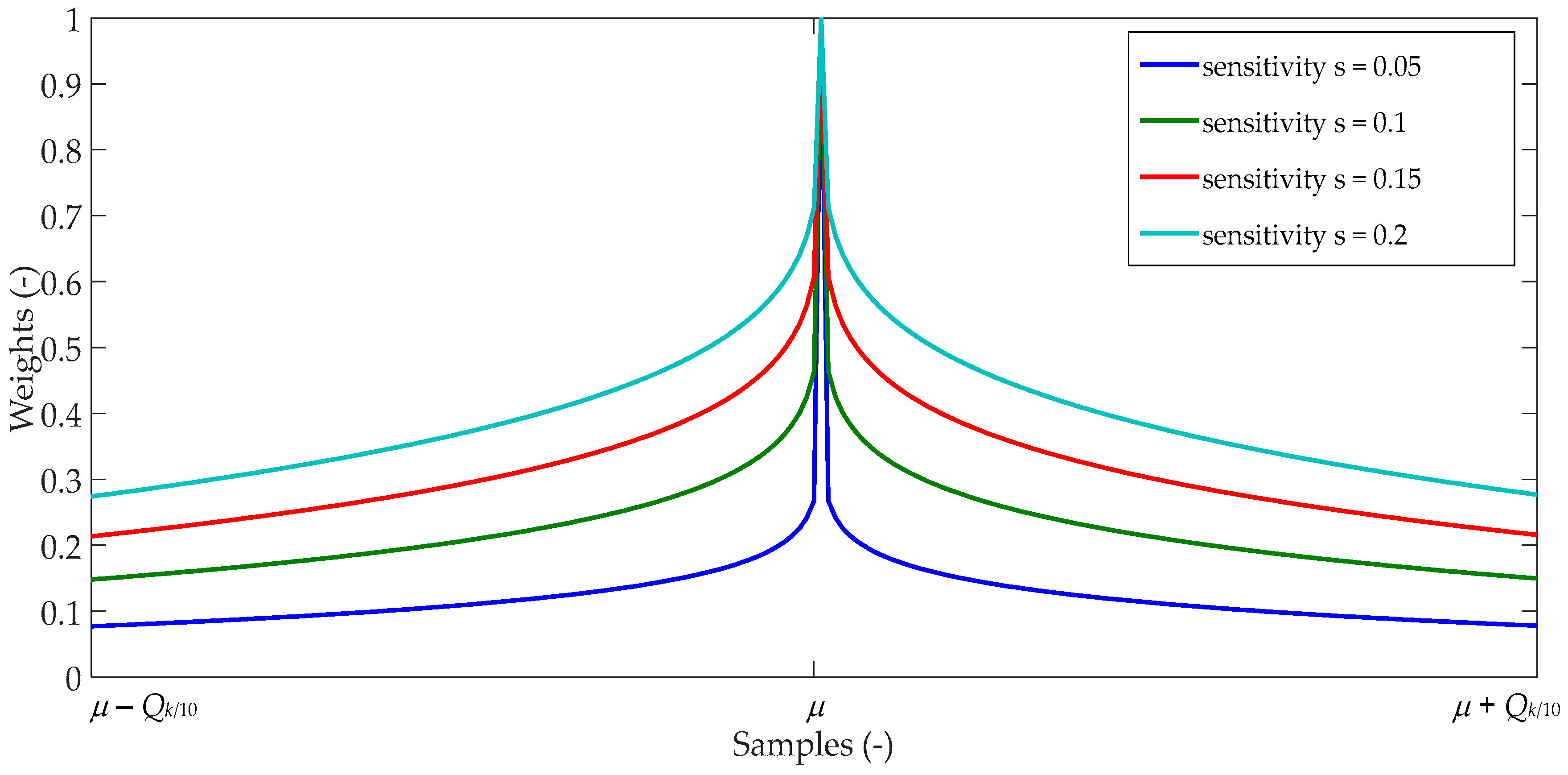
μ. The Power function in Equation (6) is not entirely appropriate for filtering because the function has the shape of a tip so the higher weights are assigned at a very narrow interval (
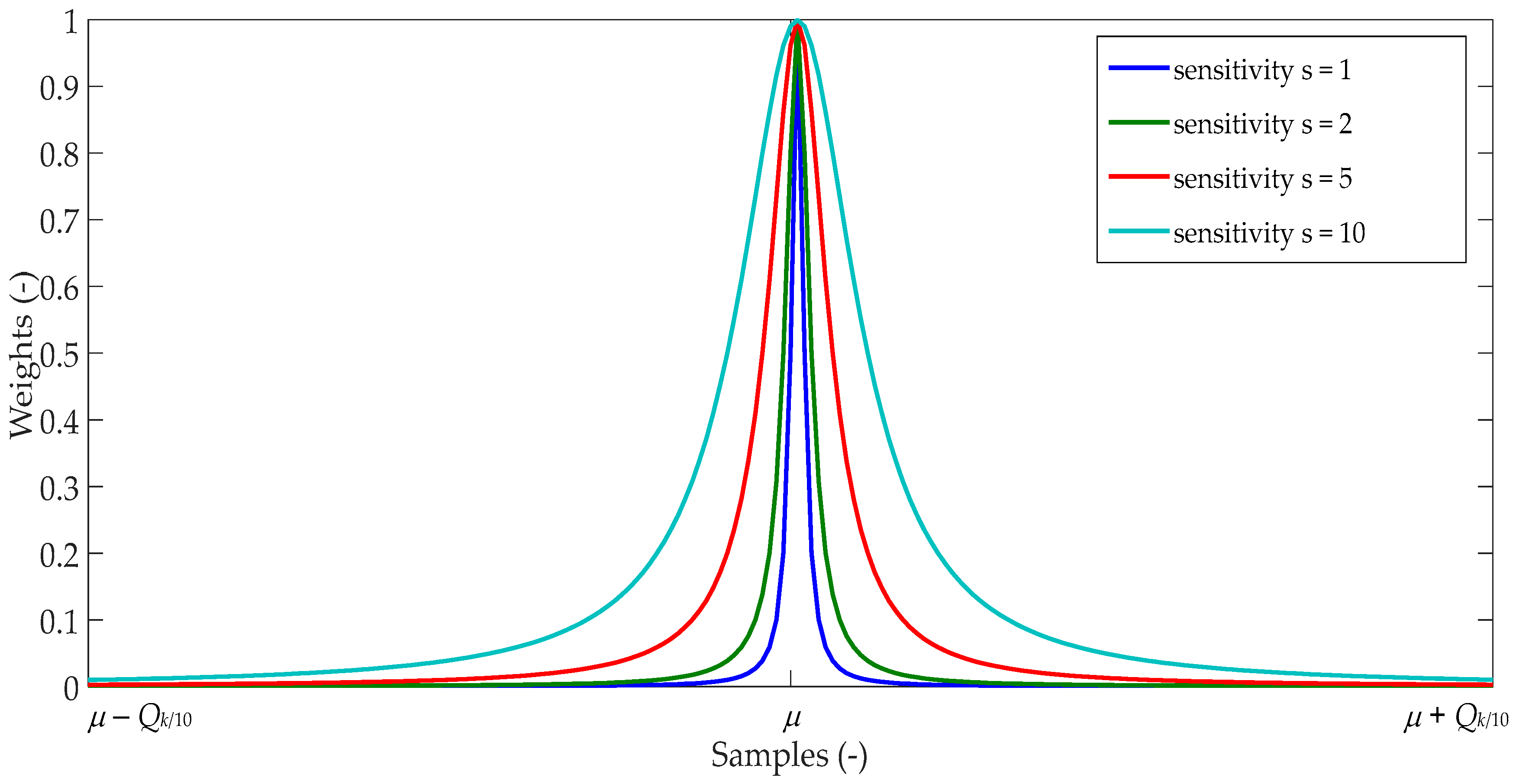
Figure 5). The Bell membership function with weights in Equation (7) has a similar behavior (
Figure 6) to the Gauss function. The main difference is the smaller width of the interval with higher weights, which seems to be useful for filtering slowly changing waveforms.
2.5. Testing of the Membership Function Filter
The model of the designed filter with the membership function was created in C programming language (Microsoft Visual C++ Express 2008 for Matlab R2007A, Microsoft Corporation, Redmond, WA, USA, 2010) and it was implemented into the Matlab Simulink (Matlab R2010a, The MathWorks Inc., Natick, MA, USA, 2010) environment as an individual block. Firstly, the model time responses to unit step were simulated for
k = 20 samples using different membership functions (
Figure 7).
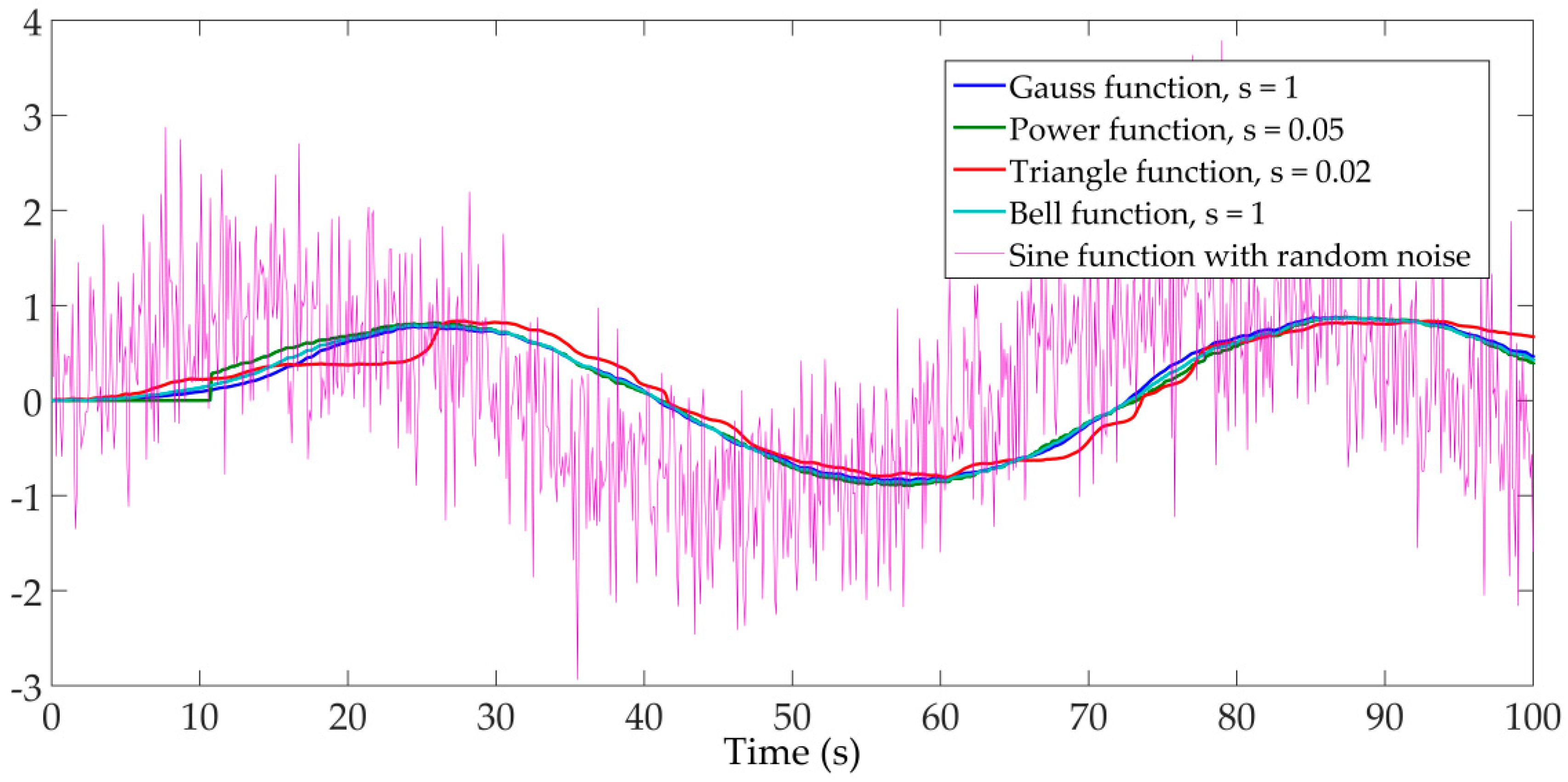
Next, the model was simulated for filtration of the sine function with random noise (
Figure 8) again for
k = 20 samples using different membership functions with the following sensitivity parameters: for the Gauss function in Equation (4)
s = 1, for the Triangle function in Equation (5)
s = 0.02, for the Power function in Equation (6)
s = 0.05, and for the Bell function in Equation (7)
s = 1.
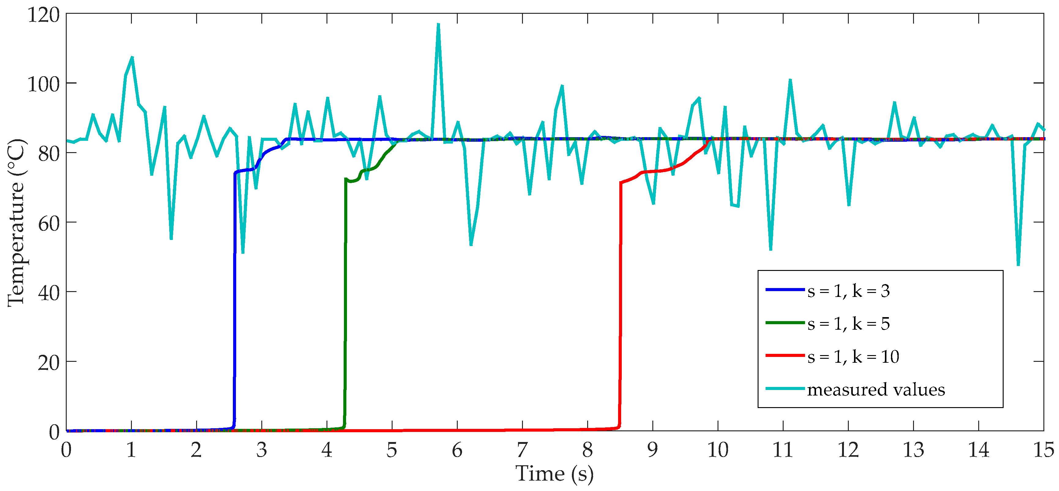
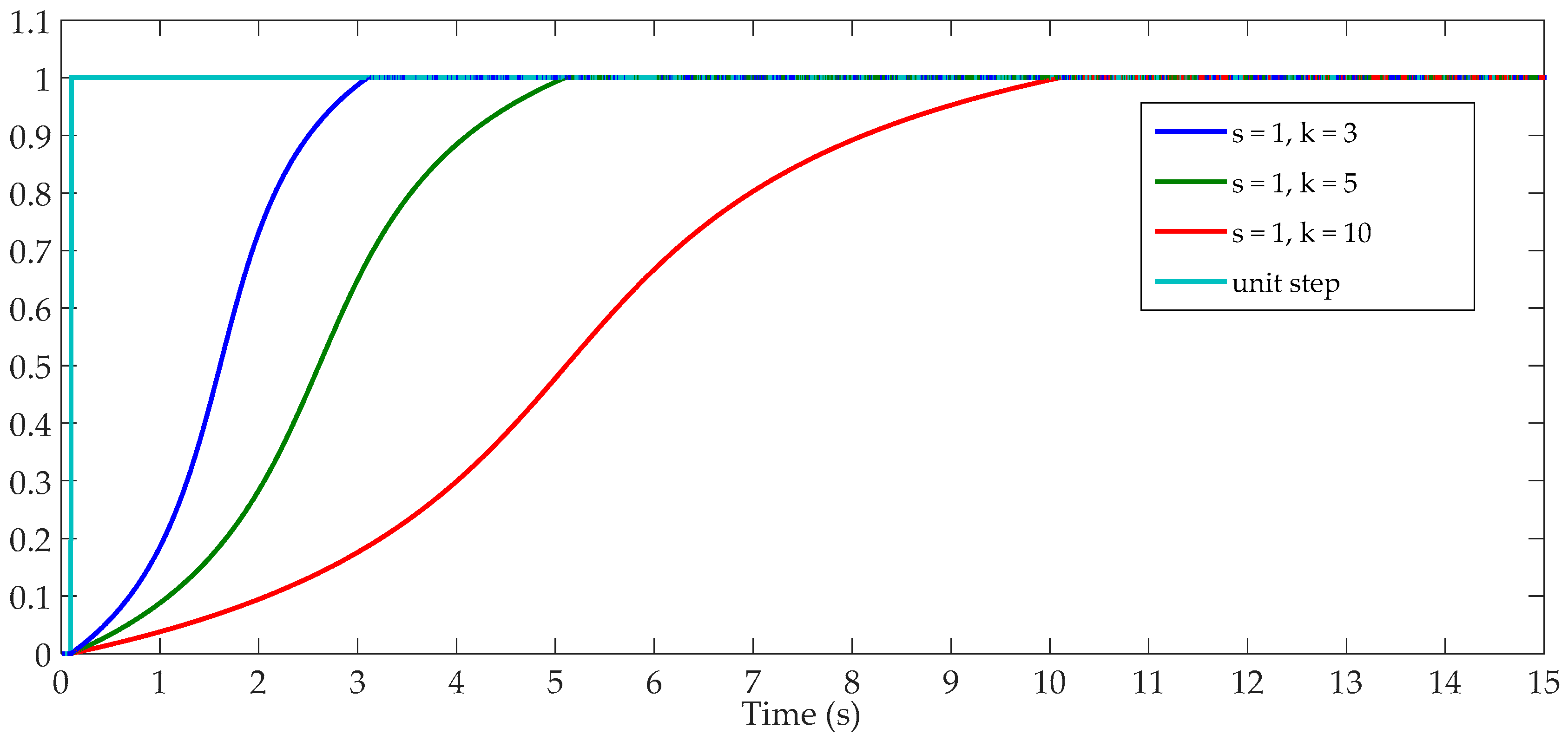
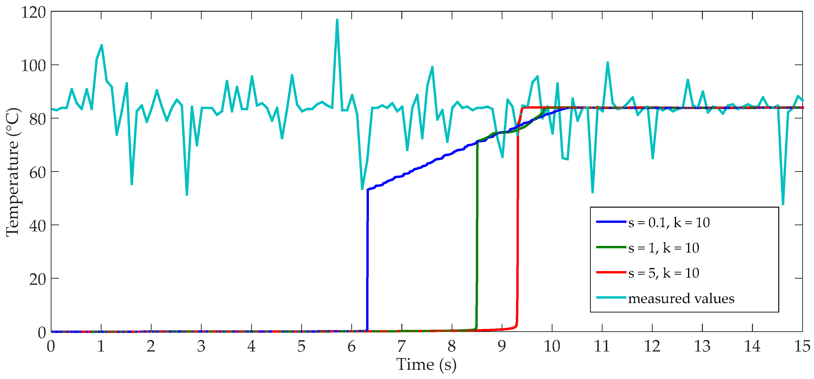
The influence of sensitivity
s and the number of samples
k were tested on a filter with the Gauss membership function. Filter time responses to unit step for different number of samples
k are in
Figure 9. The change of parameter
k can be seen in
Figure 10 as the time delay of filtration of the noisy measured temperature. The change of the membership function sensitivity
s as influenced on the filter output can be seen in
Figure 11.
3. Results
The designed filter with the Gauss membership function was implemented into a free programmable industrial process control system of biomass combustion which was monitored on-line by a Supervisory Control and Data Acquisition (SCADA) system [
11]. On-line monitoring allows visualization of the technological process (graphical schemes, diagrams, trends and reports), to evaluate the quality of combustion process and to change the control parameters with access via the internet [
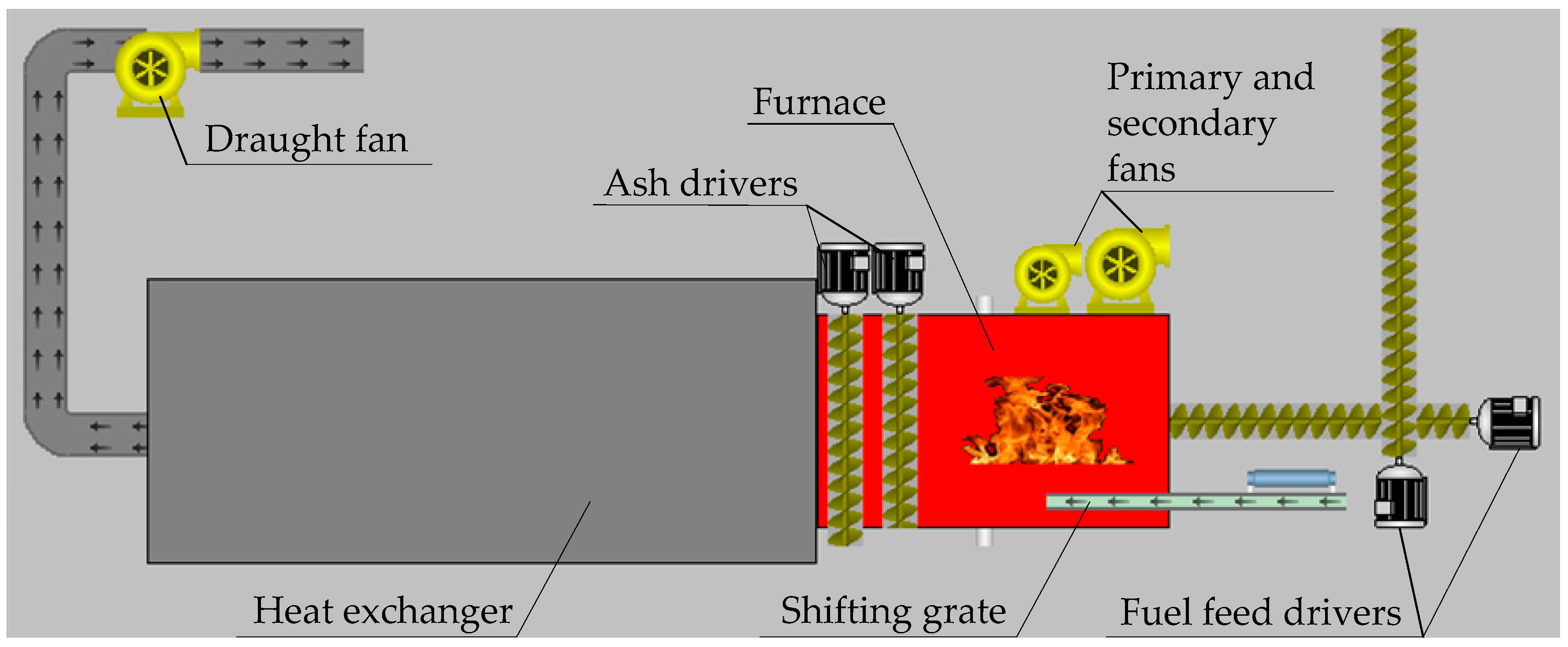
1]. The designed control and monitoring system was installed for the control of two medium-scale biomass-fired boilers for woodchip combustion (with different powers and different manufactures). Grate furnace combustion technology was used in both boilers, and the sketch of one type of boiler is in
Figure 12. The reversible shifting grate is situated in the firebox, the primary combustion air is fed by means of a fan under the grate, the secondary one above the grate. The amount of primary and secondary air is controlled by means of corresponding fan rpm [
3].
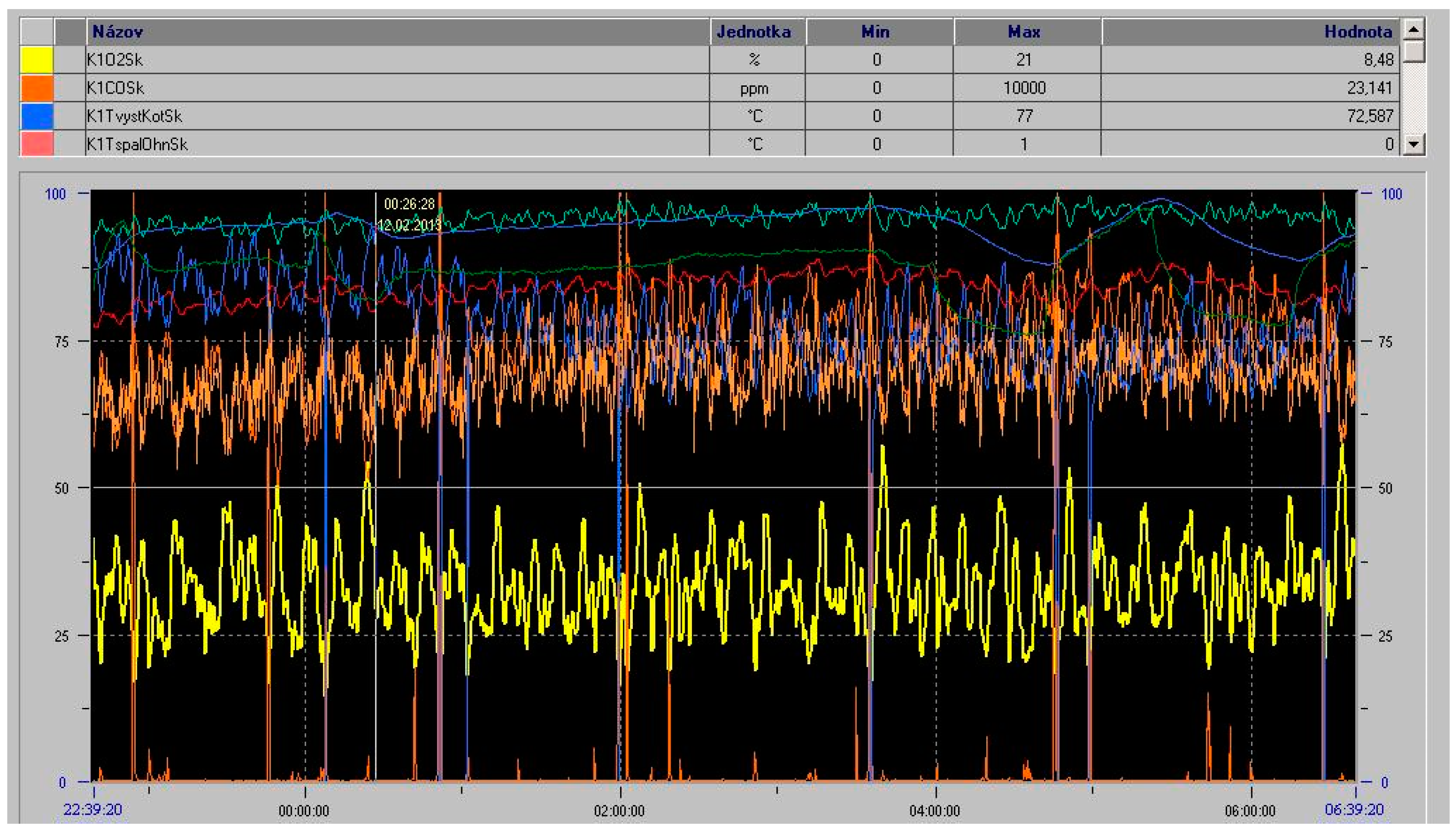
In
Figure 13 there is an example of the process variables’ remote monitoring. As can be seen, some of them are interfered with strongly. In particular the quality of O
2 concentration sensing (yellow course in
Figure 13) was unable to be used for effective control of the combustion process. The correct values of O
2 concentration in the flue gas are very important for the combustion process control because efficiency of the biomass combustion depends on the excess air ratio
λ, which can be obtained from the measured O
2 concentration as follows [
23]:
where O
2% is oxygen concentration in the flue gas in percentage.
That is why, firstly, the new filter with a membership function was applied for filtering O
2 concentration measured data and the result of filtration is shown in
Figure 14.
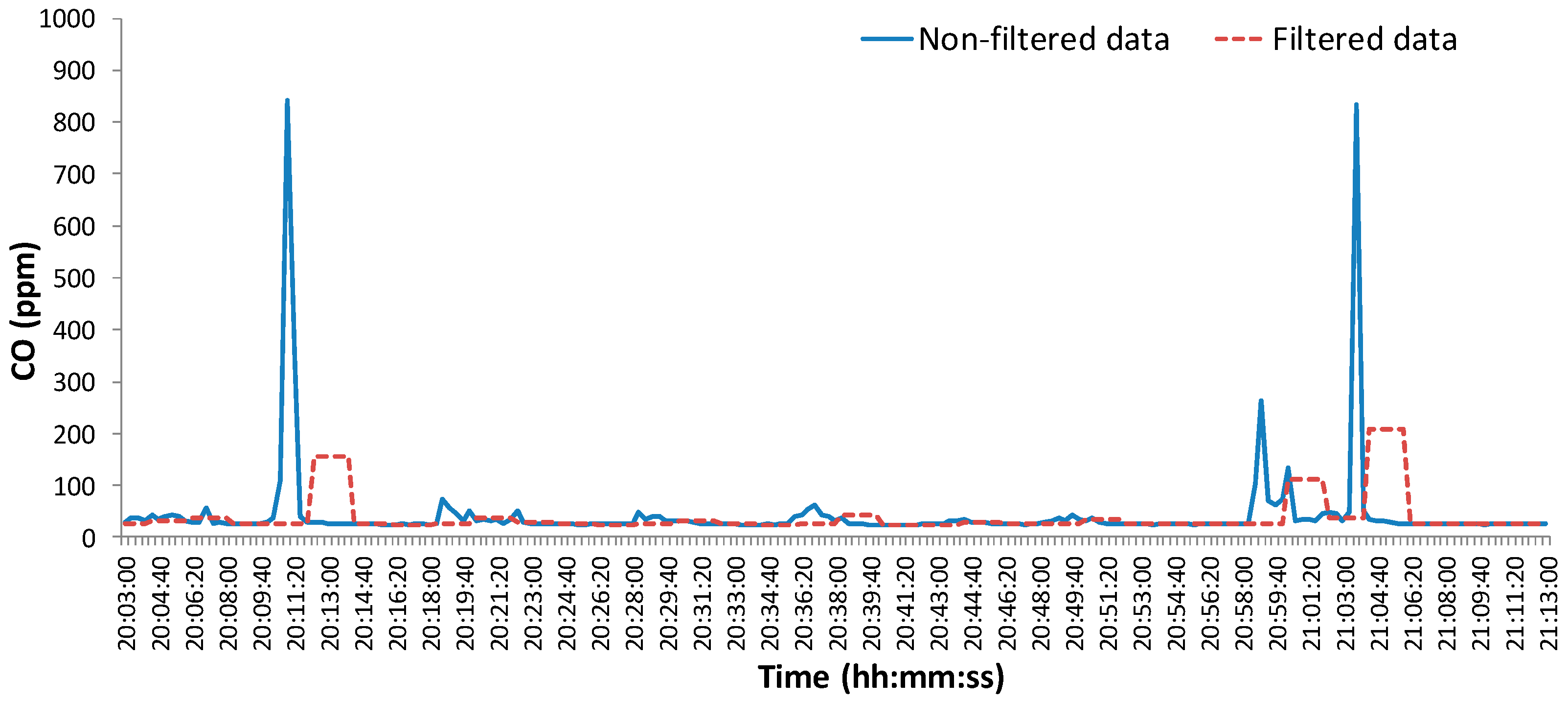
The optimal range of excess air ratio
λ for biomass combustion is usually in the interval (1.4–2) and its optimal value depends on the type of wood, the moisture content in the wood, combustion chamber construction, and so on. However, the most optimal biomass combustion operating conditions are when the compromise between maximal combustion efficiency and minimal CO emissions is achieved. One of the control algorithm’s tasks is to find such a value of excess air ratio
λ so that CO emissions would be minimal, even with the change in fuel parameters. To fulfill this task, it is necessary to continuously monitor a trend between CO emission and excess air ratio and, consequently, to change the set point of O
2 concentration in the flue gas [
11,
24]. That is why this filter was also applied for filtering CO emissions’ measured data, and the result of filtration is shown in
Figure 15.
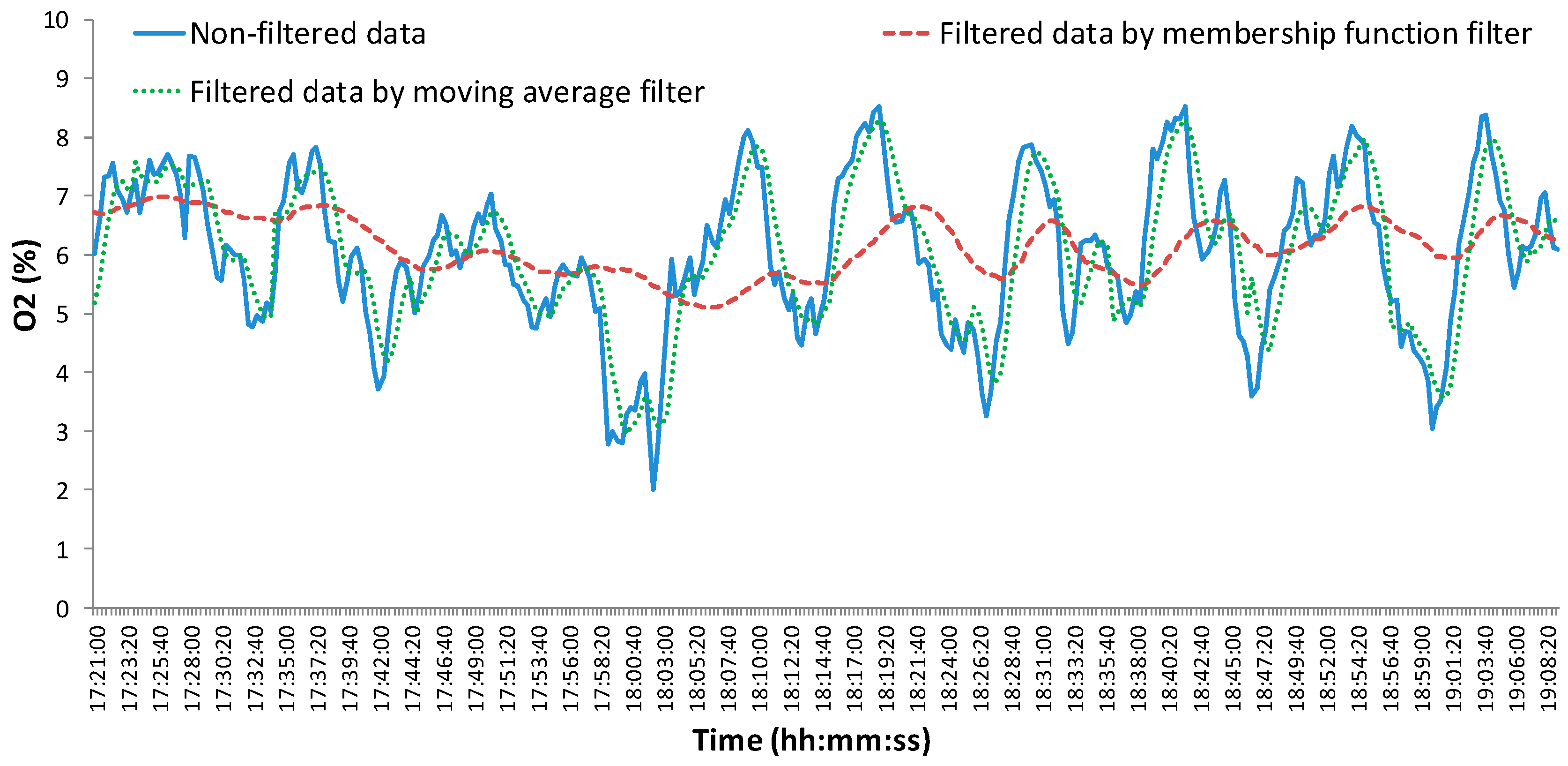
The quality of filtration has been confirmed by comparison of the membership function filter with the other types of filters.
Figure 16, for example, shows a comparison with a moving average filter. As such, it can be seen that the moving average filter does not exclude values that are extremely different. On the other hand, the membership function filter monitors the trend of data, but there is a significant time delay. However, this time delay does not have an important impact on O
2 or CO sensing in the biomass combustion process because the trend of their concentration is important not their current values.
4. Conclusions
Behavior of the membership function filter can be influenced mainly by two parameters:
- (1)
Sensitivity s of the membership function—this determines how strongly the samples near the average value are preferred, respectively, and how strongly the samples away from the average value are suppressed.
- (2)
The number of samples k used for counting of moving weighted average-higher value of parameter k causes a longer time delay of the filter, but on the other hand if k is very low the filtered data copy more real data with noise.
The filter with a normal distribution membership function was chosen for filtering important variables in the biomass combustion process. This function with appropriately selected parameters s and k ensures that the remote values from the average have lower weights (in opposite to Bell and Power function) and values which are close to the average have concave shape of weights (in opposite to Triangle function).
This was proven by implementation of the designed special filter into a control system of biomass combustion process that it is useful for signal filtering of O
2 concentration measured by a low-cost wide band Lambda probe and CO emissions measured by a simple CO sensor. The implemented filter based on the Gauss membership function with parameters set to values
k = 60,
s = 4 had a significant effect on reducing signal interferences arising in the biomass. The implemented control algorithms based on using information about the filtered tendency of nascent carbon monoxide successfully stabilized the combustion process in medium-scale biomass-based boilers, especially during the start of combustion or its interruption due to some disturbance. These advanced algorithms can also compensate for varying woodchip parameters (moisture content in wood, type and quality of wood), which is an object of intensive research at the authors’ workplace [
25].
5. Patents
Inventors: Boržíková, J., Mižák, J., Piteľ, J., Židek, K. Membership Function Filter. Patent number: SK201200021-A3.
Inventors: Balara, M., Mižák, J., Mižáková, J., Piteľ, J. Discrete Signal Weighting Average Computing Device. Patent number: SK201350050-A3.


