Investigation of the Dynamic Buckling of Spherical Shell Structures Due to Subsea Collisions


1
Department of Civil Engineering, Jiangsu University of Science and Technology, Zhenjiang 215002, China
2
Department of Civil Engineering, School of Engineering, University of Birmingham, Birmingham B15 2TT, UK
*
Author to whom correspondence should be addressed.
Appl. Sci. 2018, 8(7), 1148; https://doi.org/10.3390/app8071148
Submission received: 24 May 2018
/
Revised: 10 July 2018
/
Accepted: 12 July 2018
/
Published: 14 July 2018
(This article belongs to the Section Mechanical Engineering)
Abstract
:This paper is the first to present the dynamic buckling behavior of spherical shell structures colliding with an obstacle block under the sea. The effect of deep water has been considered as a uniform external pressure by simplifying the effect of fluid–structure interaction. The calibrated numerical simulations were carried out via the explicit finite element package LS-DYNA using different parameters, including thickness, elastic modulus, external pressure, added mass, and velocity. The closed-form analytical formula of the static buckling criteria, including point load and external pressure, has been firstly established and verified. In addition, unprecedented parametric analyses of collision show that the dynamic buckling force (peak force), mean force, and dynamic force redistribution (skewness) during collisions are proportional to the velocity, thickness, elastic modulus, and added mass of the spherical shell structure. These linear relationships are independent of other parameters. Furthermore, it can be found that the max force during the collision is about 2.1 times that of the static buckling force calculated from the analytical formula. These novel insights can help structural engineers and designers determine whether buckling will happen in the application of submarines, subsea exploration, underwater domes, etc.
1. Introduction
Deep sea submarines have been used widely in many applications such as investigation, the exploration of oceanographic resources, military action, and so on [1,2,3,4,5]. In reality, all subsea structures are subjected to significant hydrostatic pressure [6,7]. Therefore, the pressure hull is the most important component of any deep submersible. It cannot only offer the capability for resisting the external load, it can also provide more workspace for captains or scientists. The shape of the hull is usually designed as a spherical shape [8,9]. In practice, the exploration vehicle usually works at a sea depth of 1.5–8.5 km under the mean sea level with a low speed [10,11,12,13]. During operations, a collision could occur between the submarine and any obstacle such as a rock wall, iceberg, cliff, or another submarine, as shown in Figure 1. The collisions can induce the damage of the submarine nose structure through the failure of components, and the unstable deformation or buckling of the spherical nose. The buckling behavior and buckling criterion of spherical shell structures subjected to collisions have attracted more research attention over recent years [14,15,16].
Many previous studies have been carried out that investigate spherical shells under a uniform pressure [17,18,19,20]. The first and most preeminent researcher who established the buckling theory is Timoshenko [21]. His classical conclusion was derived under the elastic material and small deformation assumption. Afterwards, many studies considering large deformation and more complicated loads have been investigated [22,23,24]. Smith [25] evaluated the buckling of a multi-segment underwater hull. In his study, it was revealed that the collapse pressures from numerical analyses agreed well with all five experimental results obtained from the collapse test of a laboratory-scale mild steel structure. Zhang and Wang [26] studied the effect of thickness on the buckling strength of egg-shaped pressure hulls. The results showed that the egg-shaped pressure hulls seem to be applicable to deep sea manned/unmanned submersibles, especially to full ocean depth ones (11,000 m). Khakina [27] and Yu [28] studied the buckling load using the energy method for subsea collisions. However, they studied the static problem without dynamic effect.
It was reported that the deep pressure hull could be buckled without exceeding the limited strength under collision [29,30], which can be strongly affected by the shell thickness, collision velocity, and properties of materials [31,32]. Nevertheless, spherical pressure hulls are the most efficient and popular type for the deep-sea pressure hull structures [33,34,35], as the spherical hull has the lowest buoyancy factor (weight-to-buoyancy ratio) [36,37]. Liang and Shieh [38] reported the results of a numerical study on the optimal design of a multi-segment spherical hull, which contained details regarding the sensitivity analysis of the design variables, including the thickness and the inner radius of the rib-ring. Furthermore, Xu bai et al. [39] analyzed the capacity of the ring-stiffened cylindrical shell via the experimental method. The paper exhibited the influence on the stability of the cylindrical shell, but had little analytical discussion based on the derivations of the buckling loads of the cylindrical shell. Mackay et al. [40] studied the stability of submarines with and without artificial failure. Several numerical models to evaluate stability were established, but whether or not the results could be extended to the other applications was not discussed. Bich et al. [41] analyzed the nonlinear static and buckling of spherical shells under external pressure, incorporating the effects of temperature. They took von Karman-Donnell geometrical nonlinearity and the external pressure load without a concentrated load into account.
Based on the critical literature review, it appears that very few studies exist for the spherical shells that consider both external pressure and collision [42,43,44]. Therefore, this present paper is the first to reveal the dynamic buckling behavior for spherical shell structures experiencing the hydrostatic pressure and the concentrated dynamic force induced by subsea collision. This study employs ANSYS18.0 and LS-DYNA to establish the static and dynamic models, respectively. Parametric analysis has been carried out to determine and validate an explicit formulation for static critical buckling load. To obtain the relationship between dynamic buckling force and the static buckling force, the max and mean dynamic force over the duration of the collision are analyzed. The effects of the material and geometrical properties, external pressure, and added mass of the spherical shells are then investigated and discussed.
2. Static Buckling Criteria
2.1. Static Buckling Criteria
From the introduction above, the buckling critical pressure of the spherical shell under a uniform external pressure load based only on the elastic material can be written as Equation (1) [45]:
where , are the elastic modulus and the Poisson ratio of the materials, respectively. and are the thickness and the radius of the shell, respectively. However, surprisingly, it is important to note that there is no buckling critical force for the spherical shell under concentrated load only.
By defining p* in Equation (2), where p is the concentrated load, it can be found [45] that the slope of reaction force–deflection curve changed rapidly at around p* = 2.0. Thus, there is no analytical buckling critical load for the spherical shell under both external pressure and concentrated load [46,47,48,49]. From the report [45] mentioned above, the critical force as a critical point load situation can be defined by p* = 2.2. Clearly, the critical point load varies with different pressure, so that the buckling criteria is the function of both point load and external uniform pressure . In this paper, the critical formulation can be expressed as Equation (3), satisfying two limitations:
2.2. Verification of FEM Model
The evaluation result of the spherical shell under concentrated load is shown in Figure 2, which can be verified by the FEM model. The model is based on a perfect hemispherical shell with a radius of 5 m and a thickness of 0.1 m. The displacement has been applied at the apex of the shell, with the bottom of the shell fixed in all of the X-Y-Z directions, as shown in Figure 2a. The ideal elastic–plastic model has been adopted as the constitutive model in which the elastic modulus is 210 GPa, the yield stress is 750 MPa, and the Poisson ratio is 0.23, as shown in Figure 2b. The Shell181 element in ANSYS 18.0 is used with the large displacement option on. Figure 2c shows a comparison plot of the reaction force of the apex versus the deflection ratio, where the deflection ratio was defined as , and p* was defined as shown in Equation (2).
Figure 2c shows the comparison of the reaction force at the apex point versus the corresponding displacement between the numerical data and experimental results from Sabir [49]. In order to demonstrate the influence of the discretization, the numerical result with different meshing size is displayed. Since the results of size = 0.3 m and size = 0.1 m are the same, the size 0.3 m has thus been adopted in this paper. It can be concluded that the results agree very well, and the result trend is not linear or bilinear, but rather is irregular. At the beginning, the slope is steep, and after p’ at around 2.2, the slope becomes very mild. Thus, the value of can be defined by p* = 2.2.
2.3. Static Simulations
2.3.1. Model
Several numerical simulations have been conducted to validate the precise expression of buckling formulation and the relevant parameters by regression analysis. The models have simulated identical parameters to the initial studies with thicknesses of 0.05 m and 0.10 m, respectively. In order to obtain the critical load data, including pressure and point load, the different uniform pressure and displacement have been applied 1.0 m at the apex [52,53,54]. The bottom of the shell is set to be fixed, as shown in Figure 2a.
Figure 3 shows the typical results of reaction force versus the corresponding displacement. When the displacement is at 0.10 m, the reaction force reaches its maximum value. Then, it decreases with the increment of displacement, implying that the shell has been buckled. Note that the point load has to be in the inverse direction (negative value) in order to enable the large deformation. The buckling load can be obtained as p = 9.8 MN with q = 16 MPa. In addition, the von Mises stress at the apex versus the displacement is depicted in the same figure. The maximum stress is about 415 MPa, which is less than the yield stress, considering that the structure may be failed for either exceeding the limited strength or buckling without exceeding the limited strength, so that the material behaves as an elastic model before buckling.
2.3.2. Results
2.3.3. Regression Analysis
Figure 4a–d shows the relationship of reaction force versus pressure, according to the data of Table 1 and Table 2. In order to obtain the precise function, the results are fitted based on the same function by using the regression analysis method. It can be obtained that the function of Equation (3) can be written as Equation (4) with two parameters of , , which satisfy the limitation of Equation (3) totally when < 0,
2.4. Buckling Criteria Analysis
All of the results of regression analyses are shown in Table 3. The average values of and are 0.208 and 0.875. For convenience in application, the parameters of Equation (5) can be admitted as = 0.2 and = −0.9.
2.5. Discussion on Static Buckling
According to the results of Table 3, Equation (4) can be re-written as Equation (5). It should be noted that when the force and pressure satisfy the formula in Equation (5), the static buckling will incur. The pressure tends to be an infinite value, as the pressure tends to be zero. In such a case, the buckling force does not exist if the pressure is very small. Similarly, Sabir [49] also showed that when < 0.05, the buckling would not be induced.
3. Dynamic Buckling Criteria
3.1. Model
The dynamic model has been established by using two segments, including a spherical shell and a cylinder, as depicted as Figure 5a. The nose structure of the submarine can be simplified as a model of a spherical shell with added mass, as illustrated as Figure 5b. The obstacle block in both models has been simulated by solid elements. The shell structure of the submarine nose is modeled using shell elements in LS-DYNA [55]. The material for the obstacle block is set to be the rigid material with E = 35 GPa and a density of 2400 kg/m3. For the cylinder, it is usually reinforced by ring bars, a stiffener, or other measures. It is also considered as a rigid body with a thickness of 0.04 m and a density of 7800 kg/m3. The spherical shell in both models is assumed to behave as an elastic material with E = 210 GPa and a density of 7800 kg/m3. The added mass is set to 35,800 kg, which can be calculated from the total mass of the cylinder model. In addition, the effect of the strain rate was neglected in this study on the basis of the low velocity impacts. In the modeling, the radius of the shell is set to be 2.0 m, with a thickness of 0.03 m and an external pressure of 20 MPa, which implies that the submarine is considered to be in operations at the depth of 2.0 km under the sea.
The external pressure can be calculated by Equation (6):
where , , and are the density of water and gravity acceleration and the height under the sea, respectively. The pressure is then applied to the surface of the shell, as illustrated in Figure 5a,b. The initial velocity was set to be in the Z direction, which is normal to the rigid block. Since the shell structure is not a closure surface, there should be a concentrated force applied together with the added mass to resist the external pressure. The total force value was . Figure 6a,b shows the details of the meshes for both models. There are 7935 shell elements and 2600 solid elements after optimal meshing. Since the pressure load exists at all times, the static analysis under the pressure will only be carried out as the precursor prior to the dynamic analysis in LS-DYNA [56,57,58].
3.2. Comparison of Two Models
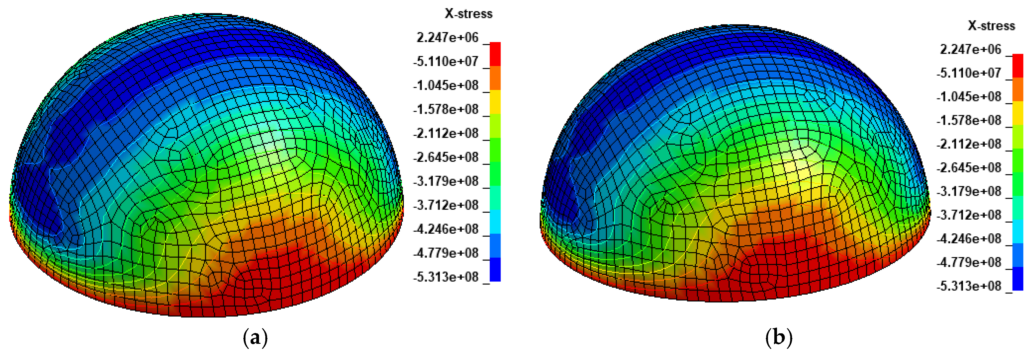
Figure 7 shows the initial state of X-stress, which is caused by the static pressure only without the time effect. Figure 7a shows the X-stress of the cylinder model, while Figure 7b shows that of the spherical shell model. It can be found that the maximum stress for each model is −648 MPa and −660 MPa (the negative sign implies that the member is in a compression state), respectively, which only has a 2.0% discrepancy. In addition, the X-stress at the apex will be = 650 MPa. The result agrees very well.
Figure 8 illustrates the displacement in the velocity direction versus time in the cases of both the cylinder and spherical shell, respectively. This figure depicts that the displacements are identical before contact (t < 0.02 s), and almost the same during the contact time (0.02 s < t < 0.06 s); lastly, it has very small discrepancy after contact (t > 0.06 s).
Figure 9 presents the time history of contact forces during collision or impact. The max forces are 17.3 MN and 17.1 MN, and the mean forces are and 9.93 MN and 9.89 MN, respectively. Therefore, it can be observed that the contact forces can be considered identical values.
Figure 10a depicts the time history of the kinetic energy. It shows that the kinetic energy is almost the same for both cases up until the half of the contact time (t < 0.045 s); then, there is some time delay (phase difference) between the cases of the cylinder model and the spherical model. After the impulse contact, the values of kinetic energy remain mostly the same (t > 0.08). Figure 10b depicts the internal energy and total energy time history of both models. It could be noticed that the internal energy of the cylinder is two times of that of the spherical shell model before collision (t < 0.02). Note that the cylinder is set to be the rigid material, so that it cannot absorb energy [59]. Nevertheless, the changing trends of the internal energy and total energy are the same.
According to the discussion above, it can be seen that all of the physical quantities of force, stress, displacement, and energy of both models could be the same. Thus, it is necessary to consider the spherical model instead of a simplified cylinder model in order to determine the dynamic buckling of the structure subjected to the collision impacts.
3.3. Relationship between Static Force and Dynamic Force
From Section 2 above, the static buckling force, including point load and pressure load, can be calculated by Equation (6). To identify the buckling under the dynamic force of collision impacts, the relationship between the static force and dynamics force should be established.
3.3.1. Methodology
In this section, the relationship between the static and dynamic force is investigated. Figure 11 illustrates the schematic plot of the calculation for the impulse, which is referred to as , the average force, which is referred to as , and the max force, which is referred to as . The average force and impulse can be calculated by Equation (7) as follows:
where and are the beginning and end of the collision procedure, , and is the contact force, which is the variable with respect to time during the contact. The skewness of the contact force is measured by . The ratio between the max and mean force represents the dynamic contact load redistribution or the skewness of the dynamic collision force during the impact.
3.3.2. Parametric Effect Due to Velocity
Table 4 presents the statistical data of the dynamic forces under different velocities. The results of , the maximum force, and the average force are calculated as described above.
Figure 12 shows the relationships between forces and velocity simulated under various cases of thickness at 0.04 m and 0.06 m. Figure 13 shows the time history of forces for the cases of impact velocities of 12 m/s, 14 m/s, and 16 m/s, respectively. It should be noted that when the velocity is larger than 14, the shell structure can be considered to be buckled already. According to Figure 13 and Table 4, the duration and impulse of collision contact is almost the same before buckling, and the skewness ratio of is almost the same as well, which implies that the contact forces have the same shape functions under a variety of impact velocities.
In addition, it can be observed that the maximum force and the mean force during collision are proportional to the velocity before dynamic buckling incurs, and the impulse is also proportional to the velocity. To identify the skewness ratio, both the maximum force and the mean force can be written in the same function as Equation (8) with different coefficients:
where and are the proportional ratio. The results of regression analysis are shown in Table 5. The skewness can be descripted by the ratio of , which can be considered as a constant value of 1.70. On this ground, it can be concluded that the maximum force and the average force comply with the same rules, and the ratio is dependent on the thickness. Moreover, the ratios of and in different cases of t = 0.06 m and 0.04 m are 1.5 and 1.6, respectively, which are almost the same as the identical ratio over the corresponding thickness. It is important to note that Equation (8) is independent of the other parameters.
3.3.3. Parametric Effect Due to Thickness
The simulations are carried out using the identical parameters with the radius of 2.0 m, the elastic modulus of 210 GPa, a Poisson ratio of 0.15, the external pressure of 15 MPa, and the different thickness parameters of 0.03 m, 0.04 m, 0.05 m, and 0.06 m, respectively. For the case of a small thickness of 0.03 m, the impact velocities are set to be 1.0 m/s and 2.0 m/s, whilst in the other cases, the velocities are set to be 4.0 m/s and 8.0 m/s.
Table 6 presents the relationship between the contact force and the thickness. It should be noted that the impact duration is different in each case of thickness, since the shell thickness can change the contact stiffness. To compare the effect of the shell thickness, the contact forces due to an impact velocity of 1.0 m/s are visualized over the data derived from an impact velocity of 4.0 m/s, as illustrated by Equation (6) and Table 4 (previously discussed in Section 3.3.2).
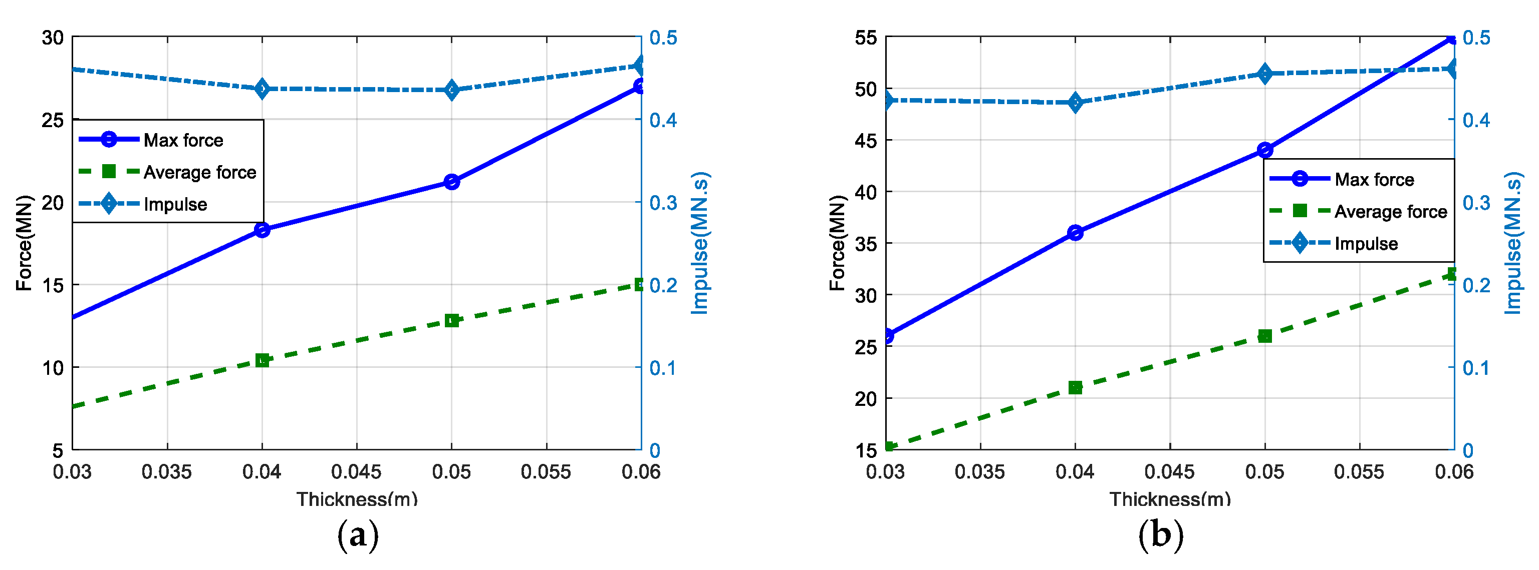
Figure 14a shows the relationship between force versus impulse and the shell thickness considering the velocity of 4.0 m/s. Figure 14b shows the same for the velocity of 8.0 m/s. It can be seen that the impulse is almost the same, despite the differences in impact duration. It can be found that the relationship can be expressed as a linear relation as written in Equation (9), considering the results from the various conditions shown in Table 7, where, and are the coefficients of maximum force and mean force, and and are a constant. When the impulses are almost identical, it is noted that the higher the max force, the shorter the time duration.
According to the results shown in Table 7, it can be found that the ratio of to can be considered as a fixed value at 1.70, which is the average value of 1.72, 1.69, 1.67 and 1.72; thereby, the maximum force and the mean force can be expressed using an identical formulation, . Furthermore, it can be established that the contact forces during collisions have an identical shape function, despite the differences in shell thickness. The ratios of to under different cases of v = 4.0 and 8.0 m/s are 0.47 and 0.48, respectively, which are almost identical to the ratio of the corresponding velocity. Thus, it can be evident that Equation (9) is independent of the other parameters.
3.3.4. Effect of Elastic Modulus and External Pressure
Numerical simulations have been carried out for evaluating the effects of elastic modulus and external pressure. The shell models have adopted the radius of 2.0 m, a Poisson ratio of 0.15, the external pressure of 15 MPa, the velocity of 3.0 m/s, and thicknesses of 0.04 m and 0.05 m, with a variety of elastic moduli and different pressures, respectively. Note that is the elastic modulus ratio, which is defined as .
Table 8 presents the relationship between the contact forces and elastic modulus ratios together with external pressures. It should be noted that the duration time of impulse contact decreases with the incremental increase of elastic modulus (or contact stiffness), but the duration time remains the same over a variety of external pressure values.
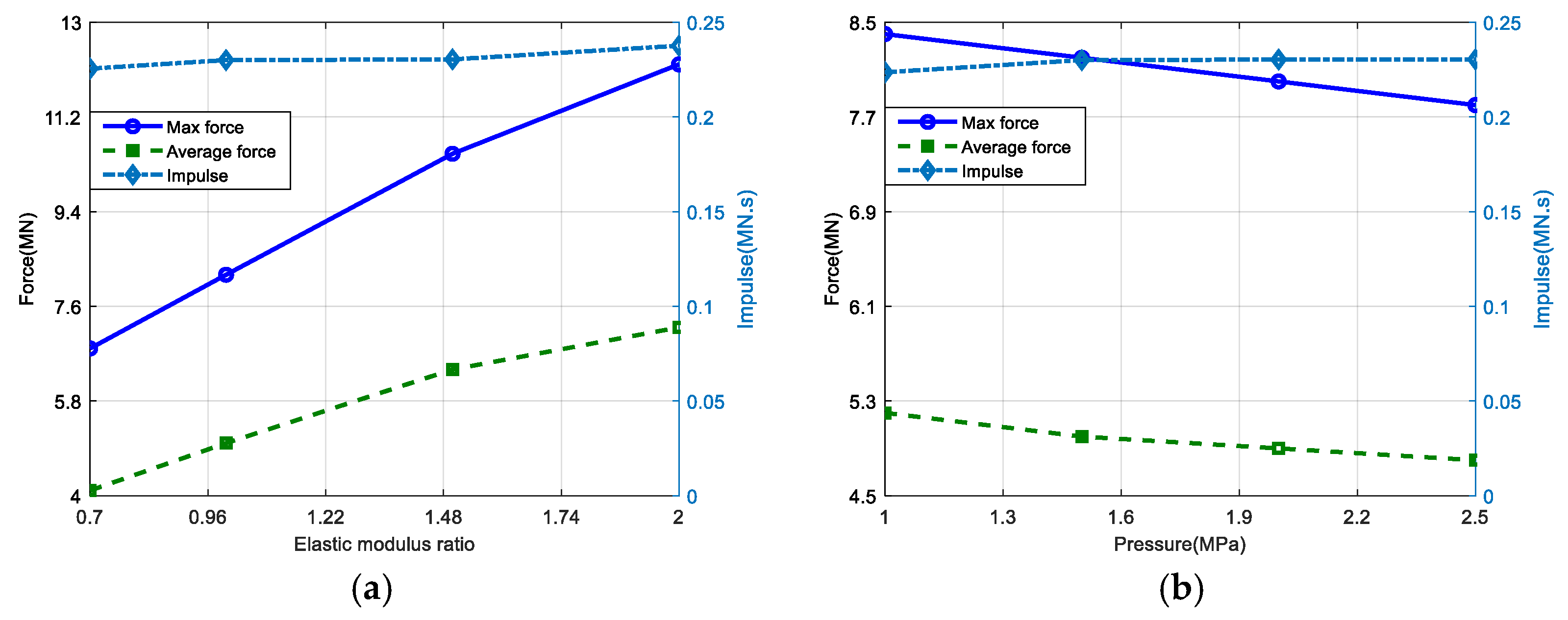
Figure 15a illustrates the relationships between force and elastic modulus ratios, while Figure 15b illustrates the relationships between forces and external pressures. Based on the results obtained, the contact forces comply with Equation (10), while the impulses remain the same over different cases. These results imply that the exchange of impact momentum for every case under various elastic modulus ratios or different external pressures is identical.
where and are the proportional coefficients. The results of regression analysis are shown in Table 9. It is apparent that the ratio of and can be considered as a constant value of 1.70, and the slope of the force over the pressure relationship is relatively very small. It can be evident that the dynamic forces are constant, regardless of the changes in external pressure. The maximum force and the mean force can be expressed in accordance with the analytical formulation, , where is 1.70 without the effect of the elastic modulus ratio. It is also clear that the contact forces during collision impacts have an identical shape function for all of the cases of the various elastic modulus ratios.
3.3.5. Parametric Effect of Added Mass
The simulations have been carried out using the shell radius of 2.0 m, a Poisson ratio of 0.15, the external pressure of 15 MPa, the velocity of 3.0 m/s, and thicknesses of 0.04 m and 0.06 m with different added mass ratios. It should be noticed that the mass ratio can be calculated as Equation (11), where is the added mass, and = 35,800 kg. The different mass ratio can simulate the different weights of the submarine.
Table 10 presents the relationship between forces and mass ratios. It should be noticed that the duration time of contact increases with the incremental increase of the mass ratio. From the regression analysis, it can be obtained that the maximum force and the mean force can be expressed in Equation (12), where the , , , and values are the proportional coefficients respective to the mass ratios.
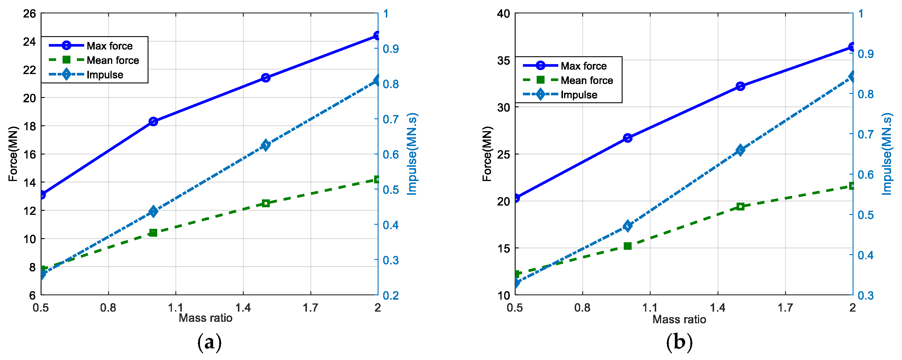
Figure 16a illustrates the relationship between the maximum force and the mean force over a variety of mass ratios, and Figure 16b illustrates the relationship of both forces versus external pressures. It is apparent that both the maximum force and the mean force comply with a linear function, as expressed by Equation (12). In addition, the ratios of and are almost the same value of 1.70. It can be observed that in the cases of different added masses, the contact forces have an identical skewness ratio. Furthermore, the ratios of and in different thickness cases of t = 0.04 meters and t = 0.06 meters are 0.6 and 0.66 respectively, which are almost identical to the ratios of the corresponding thicknesses. Thus, it can be concluded that Equation (12) is independent of the other parameters.
3.3.6. Contact Force Principle
Based on the results obtained earlier, the average force during the collision contact is proportional to the thickness and velocity, and it is linear to the elastic modulus and added mass based on the elastic material. Thus, the force can be written as Equation (13):
Combining equations (8) and (12), and taking into account the data in Table 4, Table 5, Table 6, Table 7, Table 8, Table 9, Table 10 and Table 11, the formula can be established precisely, and it can be used to solve for a variable when knowing the other parameters. Simultaneously, the collision contact forces have the almost same skewness ratio during collision. Thus, the mean force can be calculated by Equation (14):
In addition, since the contact forces in various cases using different impact velocities have the same shape function, the contact forces can thereby be descripted as Equation (15). Figure 17 shows the comparison of contact forces between the fitting results derived from Equation (15) and the numerical data. Excellent agreement can be established. Besides, according to Equation (15), the skewness ratio can be derived theoretically as = 1.57, which has a 7.6% discrepancy compared with the numerical value 1.70.
According to Equation (15), the dynamics equation can be written in Equation (16) correspondingly, where is the stiffness of the spherical shell. The relationship depends on the thickness, elastic modulus, and radius of the shell:
It can be evident that the function of displacement versus time is a harmonic function as well, and the duration time of collision depends on the thickness, elastic modulus, and density of the shell, but has little effect due to the radius and velocity of the spherical shell. This conclusion can be verified by the extensive data in Table 4, Table 5, Table 6, Table 7, Table 8, Table 9, Table 10.
3.4. Dynamic Buckling Criteria
The dynamic buckling problem can be solved if the relationship between the static buckling force and maximum force is established. In this section, the relationships between the maximum forces of collision and static buckling forces according to Equation (3) are investigated.
Figure 18 shows the X-stress of the shell under the external pressure of 15 MPa. At the beginning, the initial state is the same between the cases of velocities of 2.8 m/s and 2.7 m/s when the pressure load and configuration of the shell are the same.
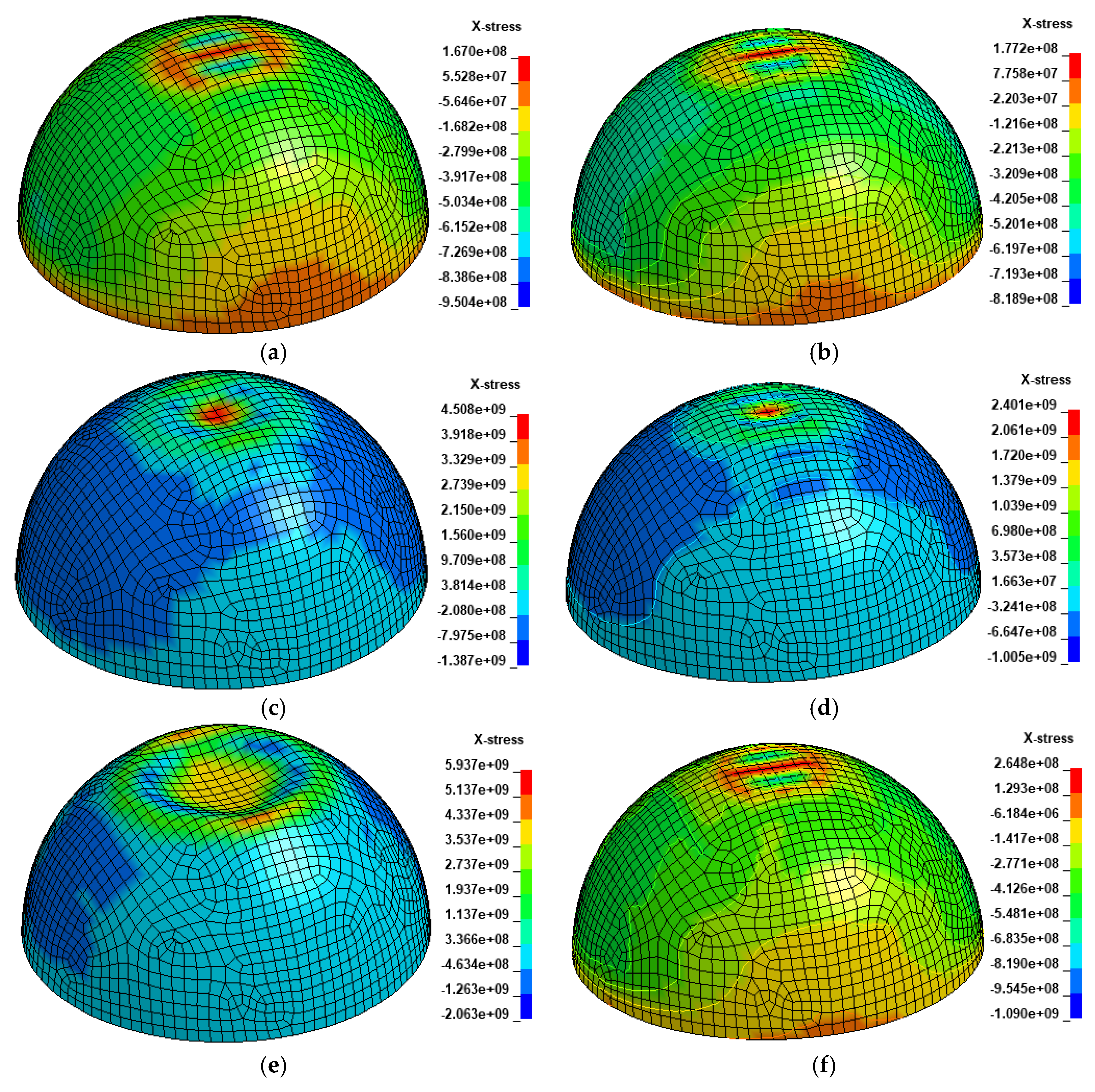
Figure 19a–h shows the mechanisms of collision for the cases with impact velocities of 2.8 m/s and 2.7 m/s. It demonstrates that in the velocity case of 2.7 m/s, the deformation of the spherical shell can be restored elastically after the collisions. However, when the velocity is larger than 2.7 m/s (even at 2.8 m/s), the deformation of the spherical shell cannot be restored after the collisions, which became larger and larger under the load of pressure and contact force. In that case, the shell can be considered to have buckled under the dynamic collisions.
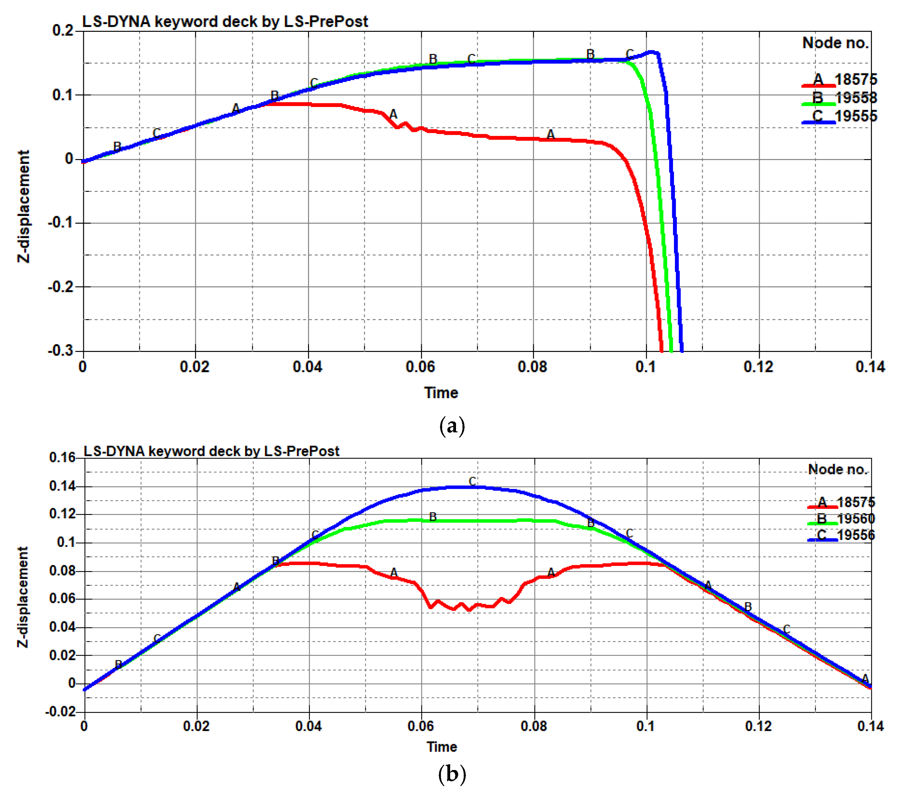
Figure 20 illustrates the Z displacement of three nodes, as previously shown in Figure 19h, which are marked as yellow spots with velocities of 2.8 m/s and 2.7 m/s, respectively. It can be found that the displacements are the same before collision contact, but they can be very different from the beginning of contact. In the velocity case of 2.7 m/s, the displacement will return back symmetrically, whilst in the case of 2.8 m/s, the displacement will return back in a steep slope (non-elastic), which implies that the shell had buckled already (the same conclusion as with Figure 19).
3.5. Dynamic Buckling Force
On this ground, the critical impact velocity Vcr can be determined to be 2.7 m/s, and according to the criteria shown above, some more critical velocities in different cases can be obtained in Table 12. It should be noted that for the application of submarines, an exploration is usually among 1.0 km to 4.5 km deep, and the external pressure is correspondingly set to be within 10 MPa to 45 MPa.
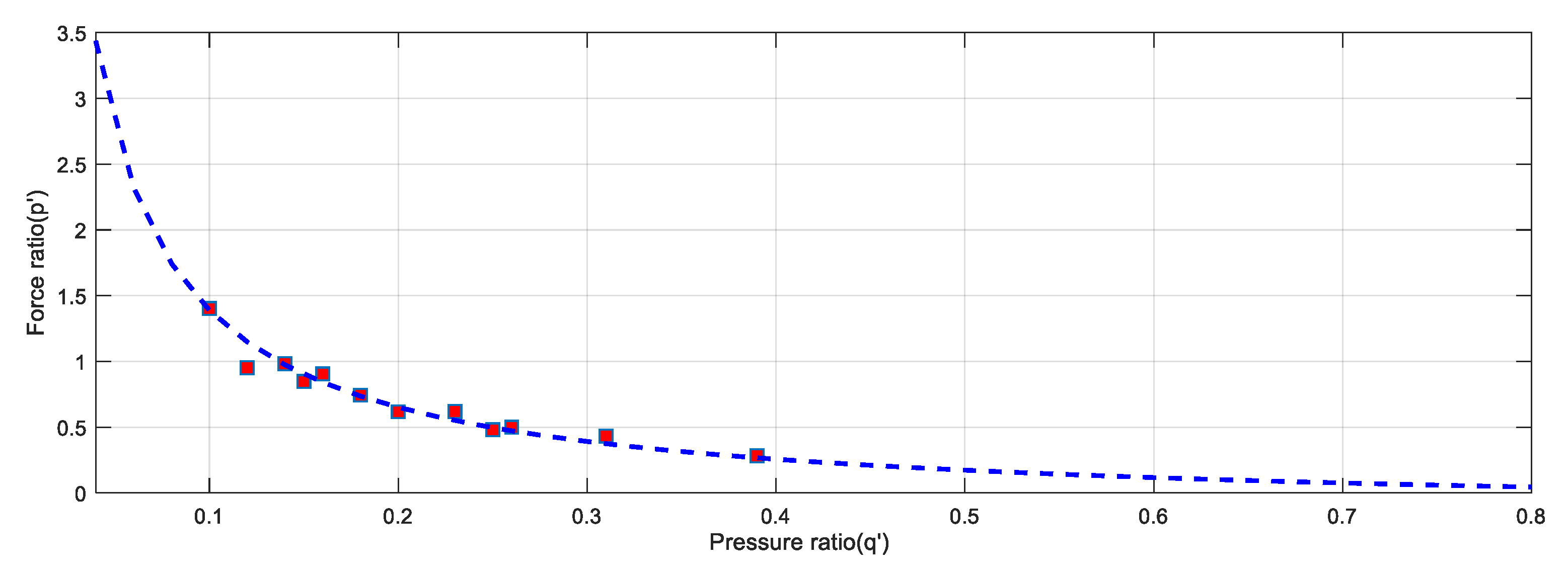
According to Table 12, the critical load in the collision can be converted into the normalized results tabulated in Table 13. Note that the labels p’ and q’ show the normalized values of pressure and maximum force respectively, according to Equation (6). The pe shows the static buckling force calculated from Equation (6) as well. The ratio is deducted by p/p’, which demonstrates the multiple of the maximum force over to the static buckling force from Equation (6).
It can be found that the maximum critical force is about 2.1 times that of the static force, inducing the dynamic buckling during the collision impacts. In summary, the critical dynamic force over the static buckling force ratios can be illustrated in Figure 21. It can also be concluded that the analytical prediction fits with the numerical simulation result very well.
4. Discussion
According to Equation (5), when the pressure tends to be zero, which means that there is no external pressure under the shell, the buckling forces can increase without boundary. Physically speaking, if the pressure ratio is less than 0.05, the force ratio would be larger than 2.8. In such a case, it can be considered that the structural buckling of the shell cannot occur.
During the collision impacts, the maximum force can be considered to be 1.70 times the average force derived from Equation (7). The impulse of collision is linear to the velocity and added mass, but has a negligible change due to the thickness and elastic modulus. In addition, the quasi-static buckling force deduced by Equation (5) is about only 0.48 times that of the maximum force during the collision. It should be noted that Equation (5) is based on the elastic material, as the buckling usually occurs before the plastic stage. The effect of strain rate is neglected for the low velocity analysis in this study. It is noted that the spherical shell could reach up to the plastic stage or over the limited stress under the collision before buckling. In that case, the structure will be damaged or failed for the lack of strength, so it is suggested that the static analysis should be analyzed before the buckling analysis.
For applications from the outcome of this study, the critical force under a single point load and a single uniform pressure load, which are named and , respectively, can be calculated firstly by Equation (1) and Equation (2) relevant to the property of the material and the parameters of the geometry. Then, the external pressure can be determined by the operation depth under the sea; therefore, Equation (5) can be used by the designer to determine the quasi-static buckling force. After obtaining the normalized force ratio of , it can be used to identify the critical velocity, which may induce the dynamic buckling by Equation (13). By the mechanism described above, the dynamic buckling of the spherical shell under the collision impacts and external pressure can be evaluated.
5. Conclusions
This paper has studied the buckling of a spherical shell structure subjected to both external pressure and point load in order to establish criteria to predict the dynamic buckling of a spherical shell structure under collision impacts. In the present study, the standard for static buckling, including external pressure and concentrated load, was established as Equation (5). Furthermore, the relationship between static force and dynamic force under subsea collisions has been studied based on the theory that the static buckling criteria can be used to reflect the dynamic collision problem. By extensive parametric analyses, a precise formulation has been formed and validated using multiple regression analyses. During the collisions, the maximum and mean contact forces are proportional to the velocity and thickness of the shell, and are also linear to the total mass and elastic modulus. For the collision impulses, they are proportional to the velocity and added mass, but the elastic modulus and shell thickness do not affect their momentum change. In addition, the same skewness ratio of the contact forces during different parameters can be considered the same value: 1.70. In that case, the contact force during collision can be descripted as a sine function with respect to time.
Overall, this study has established a fundamental framework and novel theory to simulate, design, and validate the dynamic buckling for a spherical shell structure under collision impacts and external pressure. The precise formulations shown in the present paper enable the prediction of the dynamic buckling of spherical shell structures subjected to subsea collisions. Such insights and outcomes will benefit the potential applications involving submarines and deep sea exploration, etc.
Author Contributions
L.P., S.K. and Z.D.C. developed and initialized the concept and methods; L.P. developed model and carried out analyses; S.K. provided analysis tools and validated the model; Z.D.C. and S.S.W. provided industry guidance and verified results with national standards; L.P., S.K., Z.D.C. and S.S.W. wrote and reviewed the paper; L.P. and S.S.W sought funding.
Funding
This work was supported by the national Natural Science Foundation of China (grant numbers 51508238) and by the Jiangsu Postdoctoral Research Plan (grant numbers 1601014B). The APC is sponsored by the University of Birmingham Library, U.K.
Acknowledgments
The second author wishes to gratefully acknowledge the Japan Society for Promotion of Science (JSPS) for his JSPS Invitation Research Fellowship (Long-term), Grant No L15701, at Track Dynamics Laboratory, Railway Technical Research Institute and at Concrete Laboratory, the University of Tokyo, Tokyo, Japan. The JSPS financially supports this work as part of the re-search project, entitled “Smart and reliable railway infrastructure”. Special thanks to European Commission for H2020-MSCA-RISE Project No. 691135 “RISEN: Rail Infrastructure Systems Engineering Network” (www.risen2rail.eu) [60]. In addition, the collaboration and assistance from EU Cost Action TU1409 (Mathematics for Industry Network) are highly appreciated.
Conflicts of Interest
The authors declare that there are no conflicts of interest regarding the publication of this paper.
References
- Yang, C.; Weller, S.D.; Wang, Y.X.; Ning, D.Z.; Johanning, L. Hydrodynamic response of a submerged tunnel element suspended from a twin-barge under random waves. Ocean Eng. 2017, 135, 63–75. [Google Scholar] [CrossRef]
- Figeys, W.; Ignoul, S.; Van Gemert, D. Strengthening of an industrial cylindrical shell damaged by a collision. In Structural Analysis of Historic Construction: Preserving Safety and Significance, Proceedings of the 6th International Conference on Structural Analysis of Historic Construction (SAHC08), Bath, UK, 2–4 July 2008; Taylor & Francis: London, UK, 2008. [Google Scholar]
- Kaewunruen, S.; Pompeo, G.; Bartoli, G. Blast simulations and transient responses of longspan glass roof structures: A case of London’s railway station. In Proceedings of the 25th UKACM Conference on Computational Mechanics, Birmingham, UK, 12–13 April 2017. [Google Scholar]
- Savićević, S.; Jovanović, Ž.I.J. Experimental research on machine elements of helicoidal shell shape. Tehnicki Vjesnik 2017, 24, 167–175. [Google Scholar]
- Wang, L.P.; Ayala, O.; Kasprzak, S.E.; Grabowski, W.W. Theoretical Formulation of Collision Rate and Collision Efficiency of Hydrodynamically Interacting Cloud Droplets in Turbulent Atmosphere. Am. Meteorol. Soc. 2005, 62, 2433–2450. [Google Scholar] [CrossRef]
- Ida, D.; Nakao, K. Collision of Time-Like Shells in Spherically Symmetric Spacetime. Prog. Theor. Phys. 1999, 101, 989–1000. [Google Scholar] [CrossRef] [Green Version]
- Thompson, J.M.T. Advances in Shell Buckling: Theory and Experiments. Int. J. Bifurc. Chaos 2015, 25, 1530001. [Google Scholar] [CrossRef] [Green Version]
- Bauer, S.M.; Tovstik, P.E. Buckling of Spherical Shells under Concentrated Load and Internal Pressure. Tech. Mech. 1998, 18, 135–139. [Google Scholar]
- Nash, T.J.; McDaniel, D.H.; Leeper, R.J.; Deeney, C.D.; Sanford, T.W.; Struve, K.; DeGroot, J.S. Design, simulation, and application of quasi-spherical 100 ns z-pinch implosions driven by tens of mega-amperes. Phys. Plasmas 2005, 12, 052705. [Google Scholar] [CrossRef]
- Ahn, S.S.; Ruzzene, M. Optimal design of cylindrical shells for enhanced buckling stability: Application to supercavitating underwater vehicles. Finite Elem. Anal. Des. 2006, 42, 967–976. [Google Scholar] [CrossRef]
- Chung, M.; Lee, H.J.; Kang, Y.C.; Lim, W.B.; Kim, J.H.; Cho, J.Y.; Byun, W.; Kim, S.J.; Park, S.H. Experimental study on dynamic buckling phenomena for supercavitating underwater vehicle. Int. J. Naval Archit. Ocean Eng. 2012, 4, 183–198. [Google Scholar] [CrossRef]
- Tan, C.S.; Sutton, R.; Chudley, J. An integrated collision avoidance system for autonomous underwater vehicles. Int. J. Control 2008, 7, 1027–1049. [Google Scholar] [CrossRef]
- McPhail, S.; Furlong, M.; Pebody, M. Low-Altitude Terrain following and Collision Avoidance in a Flight-Class Autonomous Underwater Vehicle. Proc. Inst. Mech. Eng. Part M J. Eng. Maritime Environ. 2010, 224, 279–292. [Google Scholar] [CrossRef]
- Qin, Q.H.; Wang, T.J. Low-velocity heavy-mass impact response of slender metal foam core sandwich beam. Compos. Struct. 2011, 93, 1526–1537. [Google Scholar] [CrossRef]
- Zhang, M.; Tang, W.; Wang, F.; Zhang, J.; Cui, W.; Chen, Y. Buckling of bi-segment spherical shells under hydrostatic external pressure. Thin-Walled Struct. 2017, 120, 1–8. [Google Scholar] [CrossRef]
- Pan, B.B.; Cui, W.C.; Shen, Y.S.; Liu, T. Further study on the ultimate strength analysis of spherical pressure hulls. Mar. Struct. 2010, 23, 444–461. [Google Scholar] [CrossRef]
- Helfer, E.; Harlepp, S.; Bourdieu, L.; Robert, J.; MacKintosh, F.C.; Chatenay, D. Buckling of actin-coated membranes under application of a local force. Phys. Rev. Lett. 2001, 87, 088103. [Google Scholar] [CrossRef] [PubMed]
- Seaman, L. The Nature of Buckling in Thin Spherical Shells. PhD Thesis, Massachusetts Institute of Technology, Cambridge, MA, USA, 1962. [Google Scholar]
- Kaplan, A.; Fung, Y.C. A Nonlinear Theory of Bending and Buckling of Tein Elastic Shallow Spherical Shells; National Advisory Committee for Aeronautics: Washington, DC, USA, 1954.
- Vető, D. Analysis of Quasi-Isometric Polygonal Buckling Shapes of Spherical Shells. Ph.D. Thesis, Budapest University of Technology and Economics, Department of Mechanics, Materials and Structures, Budapest, Hungary, 2016. [Google Scholar]
- Timoshenko, S.; Gere, J.M. Theory of Elastic Stability; McGraw-Hill International Book Company: London, UK, 1963. [Google Scholar]
- Shahandeh, R.; Showkati, H. Influence of ring-stiffeners on buckling behavior of pipelines under hydrostatic pressure. J. Construct. Steel Res. 2016, 121, 237–252. [Google Scholar] [CrossRef]
- Wang, J.H.; Zhang, W.J.; Guo, X.; Koizumi, A.; Tanaka, H. Mechanism for buckling of shield tunnel linings under hydrostatic pressure. Tunn. Undergr. Space Technol. 2015, 49, 144–155. [Google Scholar] [CrossRef]
- Yan, S.T.; Shen, X.L.; Jin, Z.J.; Ye, H. On elastic-plastic collapse of subsea pipelines under external hydrostatic pressure and denting force. Appl. Ocean Res. 2016, 58, 305–321. [Google Scholar] [CrossRef]
- Błachut, J.; Smith, P. Buckling of multi-segment underwater pressure hull. Ocean Eng. 2008, 35, 247–260. [Google Scholar] [CrossRef]
- Zhang, J.; Wang, M.; Cui, W.; Wang, F.; Hua, Z.; Tang, W. Effect of thickness on the buckling strength of egg- shaped pressure hulls. Ships Offshore Struct. 2018, 13, 375–384. [Google Scholar] [CrossRef]
- Khakina, P.N. Buckling Load of Thin Spherical Shells Based on the Theorem of Work and Energy. Int. J. Eng. Technol. 2013, 5, 392–394. [Google Scholar] [CrossRef]
- Evkin, A.Y.; Lykhachova, O.V. Energy barrier as a criterion for stability estimation of spherical shell under uniform external pressure. Int. J. Solids Struct. 2017, 118–119, 14–23. [Google Scholar] [CrossRef]
- Gish, L.A. A pseudo-coupled analytic fluid-structure interaction method for underwater implosion of cylindrical shells. Appl. Ocean Res. 2017, 66, 156–163. [Google Scholar] [CrossRef]
- Gangyi, H.; Fei, X.; Jun, L. The transient responses of two-layered cylindrical shells attacked by underwater explosive shock waves. Compos. Struct. 2010, 92, 1551–1560. [Google Scholar] [CrossRef]
- Cho, S.R.; Muttaqie, T.; Do, Q.T.; Kim, S.; Kim, S.M.; Han, D.H. Experimental investigations on the failure modes of ring-stiffened cylinders under external hydrostatic pressure. Int. J. Naval Archit. Ocean Eng. 2018. [Google Scholar] [CrossRef]
- Hutchinson, J.W.; Thompson, J.M.T. Imperfections and energy barriers in shell buckling. Int. J. Solids Struct. 2018. [Google Scholar] [CrossRef]
- Kaewunruen, S. Underpinning systems thinking in railway engineering education. Australas. J. Eng. Educ. 2017, 22, 107–114. [Google Scholar] [CrossRef]
- Huang, H.; Zhang, Y.; Han, Q. Stability of hydrostatic-pressured FGM thick rings with material nonlinearity. Appl. Math. Model. 2017, 45, 55–64. [Google Scholar] [CrossRef]
- Wang, J.H.; Koizumi, A.; Yuan, D.J. Theoretical and numerical analyses of hydrostatic buckling of a noncircular composite liner with arched invert. Thin-Walled Struct. 2016, 102, 148–157. [Google Scholar] [CrossRef]
- Yu, C.L.; Chen, Z.T.; Chen, C.; Chen, Y.T. Influence of initial imperfections on ultimate strength of spherical shells. Int. J. Naval Archit. Ocean Eng. 2017, 9, 473–483. [Google Scholar] [CrossRef]
- Lin, S.; Xie, Y.M.; Li, Q.; Huang, X.; Zhou, S. Buckling-induced retraction of spherical shells: A study on the shape of aperture. Sci. Rep. 2015, 5, 11309. [Google Scholar] [CrossRef] [PubMed] [Green Version]
- Liang, C.C.; Shiah, S.W.; Jen, C.Y.; Chen, H.W. Optimum design of multiple intersecting spheres deep-submerged pressure hull. Ocean Eng. 2004, 31, 177–199. [Google Scholar] [CrossRef]
- Bai, X.; Xu, W.; Ren, H.; Li, J. Analysis of the influence of stiffness reduction on the load carrying capacity of ring-stiffened cylindrical shell. Ocean Eng. 2017, 135, 52–62. [Google Scholar] [CrossRef]
- MacKay, J.R.; Smith, M.J.; van Keulen, F.; Bosman, T.N.; Pegg, N.G. Experimental investigation of the strength and stability of submarine pressure hulls with and without artificial corrosion damage. Mar. Struct. 2010, 23, 339–359. [Google Scholar] [CrossRef]
- Bich, D.H.; Dung, D.V.; Hoa, L.K. Nonlinear static and dynamic buckling analysis of functionally graded shallow spherical shells including temperature effects. Compos. Struct. 2012, 94, 2952–2960. [Google Scholar] [CrossRef]
- Shariati, M.; Allahbakhsh, H.R. Numerical and experimental investigations on the buckling of steel semi-spherical shells under various loadings. Thin-Walled Struct. 2010, 48, 620–628. [Google Scholar] [CrossRef]
- Hutchinson, J.W.; Thompson, J.M. Nonlinear buckling behaviour of spherical shells: Barriers and symmetry-breaking dimples. Philos. Trans. A Math. Phys. Eng. Sci. 2017, 375. [Google Scholar] [CrossRef] [PubMed]
- Zhang, J.; Zhang, M.; Cui, W.; Tang, W.; Wang, F.; Pan, B. Elastic-plastic buckling of deep sea spherical pressure hulls. Mar. Struct. 2018, 57, 38–51. [Google Scholar] [CrossRef]
- Penning, F.A.; Tburston, G.A. The Stability of Shallow Spherical Shells under Concentrated Load; National Aeronautics and Space Administration: Washington, DC, USA, 1965.
- Zhang, J.; Zhu, B.; Wang, F.; Tang, W.; Wang, W.; Zhang, M. Buckling of prolate egg-shaped domes under hydrostatic external pressure. Thin-Walled Struct. 2017, 119, 296–303. [Google Scholar] [CrossRef]
- Takla, M. Instability and axisymmetric bifurcation of elastic-plastic thick-walled cylindrical pressure vessels. Int. J. Press. Vessel. Pip. 2018, 159, 73–83. [Google Scholar] [CrossRef]
- Yan, S.; Shen, X.; Jin, Z. On instability failure of corroded rings under external hydrostatic pressure. Eng. Fail. Anal. 2015, 55, 39–54. [Google Scholar] [CrossRef]
- Sabir, A.B. Large deflection and buckling behaviour of a spherical shell with inward point load and uniform external pressure. J. Mech. Des. 1964, 6, 399–409. [Google Scholar] [CrossRef]
- Coman, C.D.; Bassom, A.P. Asymptotic limits and wrinkling patterns in a pressurised shallow spherical cap. Int. J. Non-Linear Mech. 2016, 81, 8–18. [Google Scholar] [CrossRef]
- Farhat, C.; Wang, K.G.; Main, A.; Kyriakides, S.; Lee, L.H.; Ravi-Chandar, K.; Belytschko, T. Dynamic implosion of underwater cylindrical shells: Experiments and Computations. Int. J. Solids Struct. 2013, 50, 2943–2961. [Google Scholar] [CrossRef]
- Nski, T.N.; Swiniarski, J. Numerical Calculations of Stability of Spherical Shells. Mech. Mech. Eng. 2010, 14, 325–337. [Google Scholar]
- Veto, D.; Sajtos, I. Theoretical, numerical and experimental analysis of polygonal buckling shapes of spherical shells subjected to concentrated load. J. Int. Assoc. Shell Spat. Struct. 2017, 58, 144–155. [Google Scholar] [CrossRef]
- MacKay, J.R.; van Keulen, F.; Smith, M.J. Quantifying the accuracy of numerical collapse predictions for the design of submarine pressure hulls. Thin-Walled Struct. 2011, 49, 145–156. [Google Scholar] [CrossRef]
- Livermore Software Technology Corporation (LSTC). LS-DYNA®KEYWORD USER’S MANUAL I; Livermore Software Technology Corporation: Livermore, CA, USA, 2016. [Google Scholar]
- Fan, W.; Xing, W. Deflection Solutions for Concentrated Force on Spherical Shell. In Proceedings of the 5th International Conference on Civil Engineering Transportation (ICCET 2015), Guangzhou, China, 28–29 November 2015. [Google Scholar]
- Evkin, A.Y. Large deflections of deep orthotropic spherical shells under radial concentrated load: Asymptotic solution. Int. J. Solids Struct. 2005, 42, 1173–1186. [Google Scholar] [CrossRef]
- Wunderlich, W.; Albertin, U. Buckling behaviour of imperfect spherical shells. Non-Linear Mech. 2002, 37, 589–605. [Google Scholar] [CrossRef]
- Gao, S.; Wang, X. A static spherically symmetric thin shell wormhole colliding with a spherical thin shell. Phys. Rev. D 2015, 93, 064027. [Google Scholar]
- Kaewunruen, S.; Sussman, J.M.; Matsumoto, A. Grand Challenges in Transportation and Transit Systems. Front. Built Environ. 2016, 2, 4. [Google Scholar] [CrossRef]
Figure 1.
The collision of exploration under water. (a) Exploration vehicle with ship; (b) Exploration vehicle under the sea.
Figure 1.
The collision of exploration under water. (a) Exploration vehicle with ship; (b) Exploration vehicle under the sea.
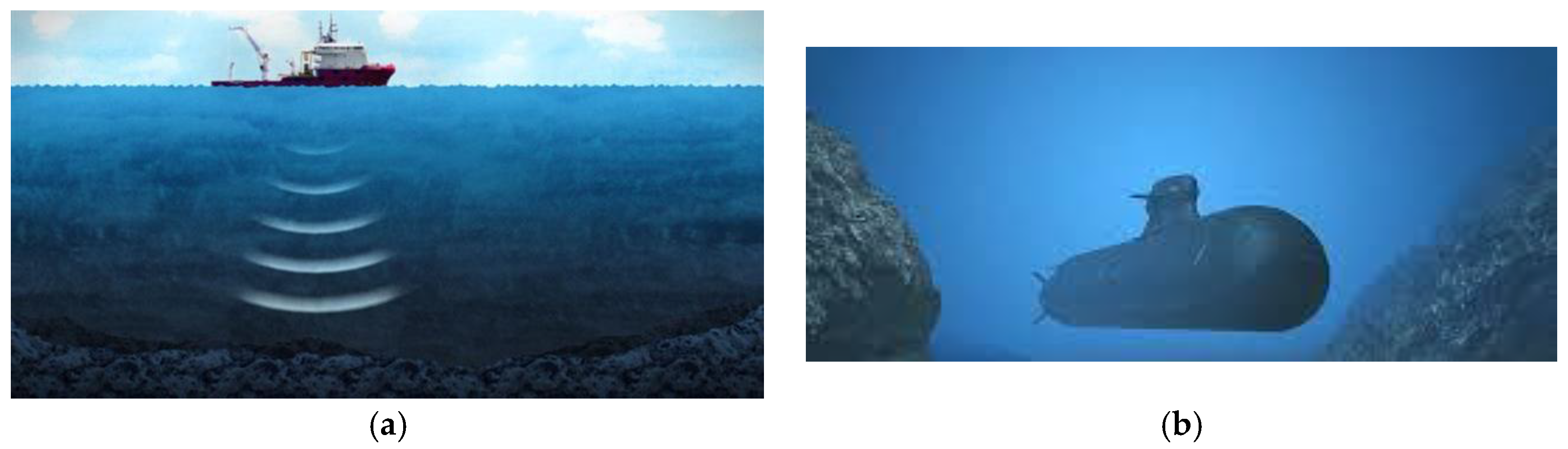
Figure 2.
The verification of the model and the result. (a) The geometry and finite element model (FEM) of structural shell for analysis; (b) The material constitutive model for FEM simulation; (c) The plot of reaction load vs. defection (0.3 m).
Figure 2.
The verification of the model and the result. (a) The geometry and finite element model (FEM) of structural shell for analysis; (b) The material constitutive model for FEM simulation; (c) The plot of reaction load vs. defection (0.3 m).
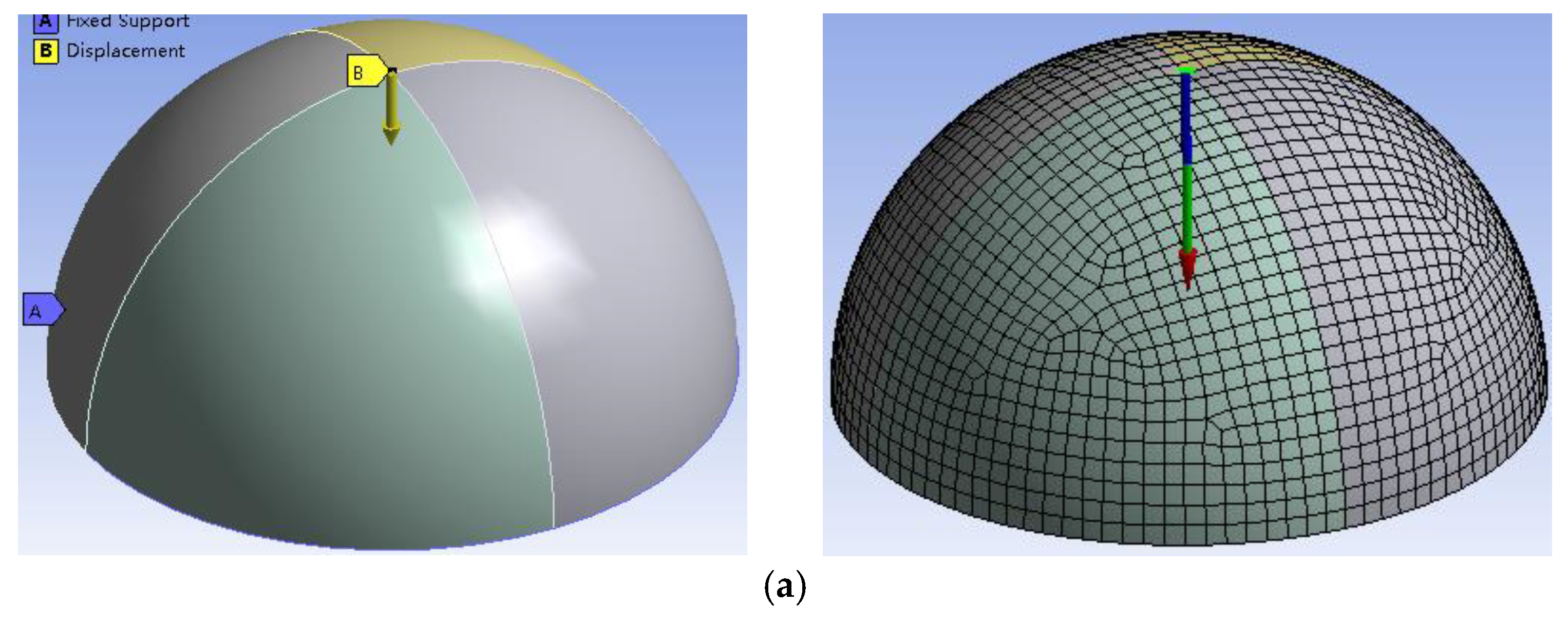
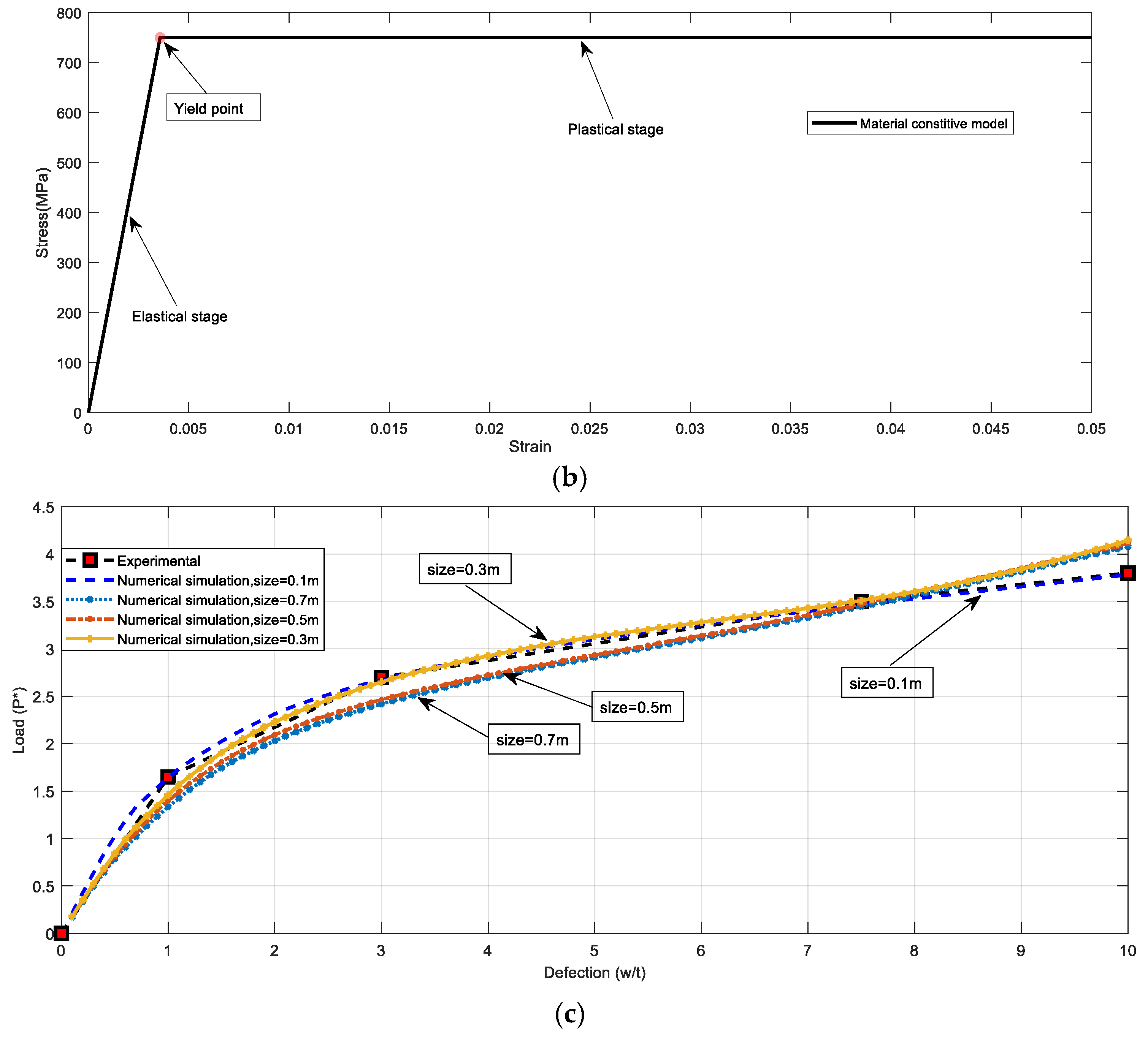
Figure 3.
The typical plot of reaction force vs. displacement.
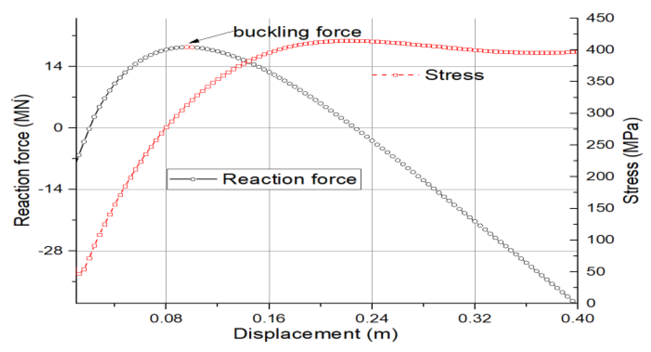
Figure 4.
The plot of reaction force vs. pressure with fitting function. (a) Case 1; (b) Case 2; (c) Case 3; (d) Case 4.
Figure 4.
The plot of reaction force vs. pressure with fitting function. (a) Case 1; (b) Case 2; (c) Case 3; (d) Case 4.

Figure 5.
The geometry and mesh model for the cylinder and spherical models. (a) The plan view of the cylinder model; (b) The plan view of the spherical model.
Figure 5.
The geometry and mesh model for the cylinder and spherical models. (a) The plan view of the cylinder model; (b) The plan view of the spherical model.

Figure 6.
The geometry and mesh model for the cylinder and spherical models. (a) The mesh of the cylinder model; (b) The mesh of the spherical model.
Figure 6.
The geometry and mesh model for the cylinder and spherical models. (a) The mesh of the cylinder model; (b) The mesh of the spherical model.
Figure 7.
The initial state of X-stress (Pa) with R = 2.0 m, t = 0.03 m, q = 20 MPa, v = 4 m/s. (a) Cylinder shell model; (b) Spherical model.
Figure 7.
The initial state of X-stress (Pa) with R = 2.0 m, t = 0.03 m, q = 20 MPa, v = 4 m/s. (a) Cylinder shell model; (b) Spherical model.

Figure 8.
The plot of displacement vs. time with R = 2.0 m, t = 0.03 m, q = 20 MPa, and v = 4 m/s.
Figure 9.
The plot of contact force vs. time with R = 2.0 m, t = 0.03 m, and q = 20 MPa.

Figure 10.
The plot of energy vs. time with R = 2.0 m, t = 0.03 m, q = 20 MPa, and v = 4 m/s. (a) Kinetic energy; (b) Internal energy and total energy.
Figure 10.
The plot of energy vs. time with R = 2.0 m, t = 0.03 m, q = 20 MPa, and v = 4 m/s. (a) Kinetic energy; (b) Internal energy and total energy.

Figure 11.
The typical plot of force vs. time.

Figure 12.
Effect of velocity on forces and impulse, with t = 0.04 m and 0.06 m. (a) t = 0.04 m; (b) t = 0.06 m.
Figure 12.
Effect of velocity on forces and impulse, with t = 0.04 m and 0.06 m. (a) t = 0.04 m; (b) t = 0.06 m.

Figure 13.
Collision force vs. time with velocities of 12 m/s, 14 m/s, and 16 m/s, and t = 0.06 m.
Figure 14.
Effect of shell thickness on forces and impulse at impact velocities of 4.0 m/s and 8.0 m/s. (a) 4.0 m/s; (b) 8.0 m/s.
Figure 14.
Effect of shell thickness on forces and impulse at impact velocities of 4.0 m/s and 8.0 m/s. (a) 4.0 m/s; (b) 8.0 m/s.

Figure 15.
Effect of elastic modulus and external hydraulic pressure on forces and impulse. (a) Force vs. elastic modulus ratio; (b) Force vs. external pressure.
Figure 15.
Effect of elastic modulus and external hydraulic pressure on forces and impulse. (a) Force vs. elastic modulus ratio; (b) Force vs. external pressure.

Figure 16.
Effect of structural mass on forces and impulse. (a) Thickness 0.06; (b) Thickness 0.04.

Figure 17.
Collision contact force vs. time with fitting result, R = 2.0 m, t = 0.06 m, q = 15 MPa, and E = 210 GPa.
Figure 17.
Collision contact force vs. time with fitting result, R = 2.0 m, t = 0.06 m, q = 15 MPa, and E = 210 GPa.
Figure 18.
The initial state of shell in the X-stress (Pa). (a) 2.8 m/s; (b) 2.7 m/s.

Figure 19.
The X-stress during contact procedure (Pa). (a) 2.8 m/s at t = 0.04 s; (b) 2.7 m/s at t = 0.04 s; (c) 2.8 m/s at t = 0.05 s; (d) 2.7 m/s at t = 0.05 s; (e) 2.8 m/s at t = 0.06 s; (f) 2.7 m/s at t = 0.06 s; (g) 2.8 m/s at t = 0.07 s; (h) 2.7 m/s at t = 0.07 s.
Figure 19.
The X-stress during contact procedure (Pa). (a) 2.8 m/s at t = 0.04 s; (b) 2.7 m/s at t = 0.04 s; (c) 2.8 m/s at t = 0.05 s; (d) 2.7 m/s at t = 0.05 s; (e) 2.8 m/s at t = 0.06 s; (f) 2.7 m/s at t = 0.06 s; (g) 2.8 m/s at t = 0.07 s; (h) 2.7 m/s at t = 0.07 s.


Figure 20.
The X displacement time history at velocities of 2.8 m/s and 2.7 m/s. (a) The case of 2.8 m/s velocity; (b) The case of 2.7 m/s velocity.
Figure 20.
The X displacement time history at velocities of 2.8 m/s and 2.7 m/s. (a) The case of 2.8 m/s velocity; (b) The case of 2.7 m/s velocity.

Figure 21.
The comparison of prediction and numerical simulation.


Table 1.
The result of criteria force with R = 5.0 m.
| Case 1 | p (MN) | q (MPa) | Case 2 | p (MN) | q (MPa) | ||
|---|---|---|---|---|---|---|---|
| t = 0.05 m E = 210 GPa ν = 0.3 | = 11.0 = 11.5 | 3.5 | 7.8 | t = 0.10 m E = 210 GPa ν = 0.3 | = 88 = 48 | 78 | 8.0 |
| 5.0 | 5.2 | 53 | 14 | ||||
| 8.9 | 2.0 | 39 | 24 | ||||
| 12 | 1.6 | 31 | 26 | ||||
| 15 | 1.35 | 26 | 32 | ||||
| 21 | 1.05 | 22 | 35 | ||||
| 26 | 0.72 | 18 | 42 |
Table 2.
The result of criteria force with R = 3.0 m.
| Case 3 | p (MN) | q (MPa) | Case 4 | p (MN) | q (MPa) | ||
|---|---|---|---|---|---|---|---|
| t = 0.05 m E = 200 GPa ν = 0.23 | = 18 = 32 | 49.2 | 1.6 | t = 0.05 m E = 500 GPa ν = 0.23 | = 45 = 80 | 75 | 10 |
| 31.5 | 3.3 | 49 | 12 | ||||
| 25.1 | 4.2 | 28 | 23 | ||||
| 16.2 | 5.3 | 23 | 34 | ||||
| 12.3 | 7.6 | 20 | 41 | ||||
| 9.6 | 12 | 13 | 60 | ||||
| 6.3 | 20 | 9.6 | 71 |
Table 3.
Fitting results of Equation (4).
| Case | 1 | 2 | 3 | 4 |
|---|---|---|---|---|
| 0.190 | 0.219 | 0.226 | 0.198 | |
| −0.919 | −0.789 | −0.811 | −0.981 |
Table 4.
The statistic of the contact forces under different cases (unit: MN, GPa, meters, s).
| Case | Vel | Case | Vel | ||||||||||
|---|---|---|---|---|---|---|---|---|---|---|---|---|---|
| R = 2.0 E = 210 ν = 0.15 t = 0.04 | 2 | 0.044 | 8.3 | 5.0 | 1.67 | 0.22 | R = 2.0 E = 210 ν = 0.15 t = 0.06 | 6 | 0.030 | 41.0 | 23.5 | 1.74 | 0.71 |
| 3 | 0.044 | 13.1 | 7.4 | 1.74 | 0.33 | 8 | 0.029 | 55.4 | 33.7 | 1.64 | 0.98 | ||
| 4 | 0.042 | 18.3 | 10.4 | 1.75 | 0.44 | 10 | 0.028 | 73.4 | 41.9 | 1.75 | 1.17 | ||
| 6 | 0.044 | 24.5 | 14.7 | 1.67 | 0.65 | 14 | 0.027 | 105 | 60.8 | 1.73 | 1.64 | ||
| 8 | 0.052 | 26.1 | 16.5 | 1.59 | 0.86 | 16 | 0.028 | 113 | 69.2 | 1.63 | 1.93 |
Table 5.
The result of regression analysis.
| Thickness | |||
|---|---|---|---|
| 0.06 m | 7.0 | 4.2 | 1.67 |
| 0.04 m | 4.6 | 2.6 | 1.73 |
Table 6.
The statistics of the contact forces in different thickness cases (unit: MN, GPa, m).
| Case | t/v | Case | t/v | ||||||||
|---|---|---|---|---|---|---|---|---|---|---|---|
| R = 2.0 E = 210 ν = 0.15 q = 15 | 0.03/1 | 0.063 | 3.07 | 1.91 | 0.12 | R = 2.0 E = 210 ν = 0.15 q = 15 | 0.03/2 | 0.062 | 5.7 | 3.5 | 0.22 |
| 0.04/4 | 0.042 | 18.3 | 10.4 | 0.44 | 0.04/4 | 0.042 | 18 | 10 | 0.42 | ||
| 0.05/4 | 0.034 | 21.2 | 12.8 | 0.44 | 0.05/8 | 0.035 | 44 | 26 | 0.91 | ||
| 0.06/4 | 0.031 | 27.0 | 15.0 | 0.47 | 0.06/8 | 0.029 | 55 | 32 | 0.93 |
Table 7.
The regression analysis into the effect of shell thickness.
| Velocity | ||||||
|---|---|---|---|---|---|---|
| 4 m/s | 449 | −0.33 | 265 | −0.38 | 1.69 | 1.69 |
| 8 m/s | 950 | −2.5 | 556 | −1.5 | 1.67 | 1.72 |
Table 8.
Results with different elastic ratios and external pressures (GPa, MN, meters).
| Case | e | Case | q | ||||||||
|---|---|---|---|---|---|---|---|---|---|---|---|
| R = 2.0 t = 0.04 q = 15 v = 3.0 | 0.7 | 0.055 | 6.8 | 4.1 | 0.23 | R = 2.0 t = 0.06 e = 1.0 v = 3.0 | 1.0 | 0.043 | 8.4 | 5.2 | 0.22 |
| 1.0 | 0.046 | 8.2 | 5.0 | 0.23 | 1.5 | 0.046 | 8.2 | 5.0 | 0.23 | ||
| 1.5 | 0.036 | 10.5 | 6.4 | 0.23 | 2.0 | 0.047 | 8.0 | 4.9 | 0.23 | ||
| 2.0 | 0.033 | 12.2 | 7.2 | 0.24 | 2.5 | 0.048 | 7.8 | 4.8 | 0.23 |
Table 9.
The regression analysis into the effect of elastic moduli and external pressure.
| Thickness | Remark | ||||||
|---|---|---|---|---|---|---|---|
| 0.04 m | 4.2 | 4.0 | 2.4 | 2.4 | 1.75 | 1.67 | Elastic |
| 0.06 m | −0.4 | 8.8 | −0.26 | 5.4 | 1.67 | 1.72 | Pressure |
Table 10.
The statistic of force in different cases (unit: MN, GPa, meters).
| Case | Case | ||||||||||
|---|---|---|---|---|---|---|---|---|---|---|---|
| t = 0.04 R = 2.0 E = 210 v = 4.0 | 0.5 | 0.033 | 13.1 | 7.8 | 0.26 | t = 0.06 R = 2.0 E = 210 v = 4.0 | 0.5 | 0.027 | 20.3 | 12.2 | 0.33 |
| 1.0 | 0.042 | 18.3 | 10.4 | 0.44 | 1.0 | 0.031 | 26.7 | 15.2 | 0.47 | ||
| 1.5 | 0.050 | 21.4 | 12.5 | 0.63 | 1.5 | 0.034 | 32.2 | 19.4 | 0.67 | ||
| 2.0 | 0.057 | 24.4 | 14.2 | 0.81 | 2.0 | 0.039 | 36.4 | 21.6 | 0.84 |
Table 11.
The result of regression analysis on Equation (12).
| Thickness | ||||||
|---|---|---|---|---|---|---|
| 0.04 m | 7.4 | 10 | 4.3 | 5.9 | 1.72 | 1.69 |
| 0.06 m | 10.8 | 15.5 | 6.5 | 9.0 | 1.67 | 1.72 |
Table 12.
The criteria velocity statistic (MPa, MN, meters, m/s).
| Case | q | Vcr | Max Force | Case | q | Vcr | Max Force | Case | q | Vcr | Max force |
|---|---|---|---|---|---|---|---|---|---|---|---|
| t = 0.04 R = 2.0 E = 210 | 10 | 16 | 45/3.0 | t = 0.04 R = 1.5 E = 210 | 30 | 9.3 | 30/1.5 | t = 0.04 R = 2.5 E = 210 | 10 | 7.1 | 23/2.0 |
| 15 | 9.8 | 26/1.7 | 45 | 6.9 | 20/1.0 | 15 | 4.2 | 16/1.3 | |||
| 20 | 6.7 | 20/1.3 | 20 | 15 | 40/2.0 | 20 | 3.3 | 11/1.0 | |||
| 25 | 5.1 | 17/1.0 | 25 | 10 | 34/1.7 | 25 | 2.2 | 7.0/0.6 |
Table 13.
The ratio of criteria in the random parameters (unit: meters, GPa).
| Case | q’ | p’/pe | Ratio | Case | q’ | p’/pe | Ratio | Case | q’ | p’/pe | Ratio |
|---|---|---|---|---|---|---|---|---|---|---|---|
| t = 0.04 R = 2.0 E = 210 | 0.10 | 3.0/1.40 | 2.12 | t = 0.04 R = 1.5 E = 210 | 0.18 | 1.5/0.73 | 2.12 | t = 0.04 R = 2.5 E = 210 | 0.16 | 1.9/0.84 | 2.26 |
| 0.15 | 1.7/0.90 | 1.97 | 0.26 | 1.0/0.47 | 2.22 | 0.23 | 1.3/0.55 | 2.36 | |||
| 0.20 | 1.3/0.65 | 1.99 | 0.12 | 2.0/1.15 | 1.74 | 0.31 | 0.9/0.37 | 2.43 | |||
| 0.25 | 1.0/0.50 | 2.03 | 0.14 | 1.7/0.97 | 2.12 | 0.39 | 0.6/0.27 | 2.22 |
© 2018 by the authors. Licensee MDPI, Basel, Switzerland. This article is an open access article distributed under the terms and conditions of the Creative Commons Attribution (CC BY) license (http://creativecommons.org/licenses/by/4.0/).
Share and Cite
MDPI and ACS Style
Liu, P.; Kaewunruen, S.; Zhou, D.; Wang, S. Investigation of the Dynamic Buckling of Spherical Shell Structures Due to Subsea Collisions. Appl. Sci. 2018, 8, 1148. https://doi.org/10.3390/app8071148
AMA Style
Liu P, Kaewunruen S, Zhou D, Wang S. Investigation of the Dynamic Buckling of Spherical Shell Structures Due to Subsea Collisions. Applied Sciences. 2018; 8(7):1148. https://doi.org/10.3390/app8071148
Chicago/Turabian StyleLiu, Ping, Sakdirat Kaewunruen, Daochuan Zhou, and Shanshui Wang. 2018. "Investigation of the Dynamic Buckling of Spherical Shell Structures Due to Subsea Collisions" Applied Sciences 8, no. 7: 1148. https://doi.org/10.3390/app8071148
Note that from the first issue of 2016, this journal uses article numbers instead of page numbers. See further details here.