Asymmetric Propagation Delay-Aware TDMA MAC Protocol for Mobile Underwater Acoustic Sensor Networks

Korea Research Institute of Ships & Ocean Engineering (KRISO), Daejeon 34103, Korea
*
Author to whom correspondence should be addressed.
Appl. Sci. 2018, 8(6), 962; https://doi.org/10.3390/app8060962
Submission received: 8 May 2018
/
Revised: 1 June 2018
/
Accepted: 7 June 2018
/
Published: 12 June 2018
Abstract
:The propagation delay in mobile underwater acoustic sensor network (MUASN) is asymmetric because of its low sound propagation speed, and this asymmetry grows with the increase in packet travel time, which damages the collision avoidance mechanism of the spatial reuse medium access control (MAC) protocols for MUASN. We propose an asymmetric propagation delay-aware time division multiple access (APD-TDMA) for a MUASN in which periodic data packet transmission is required for a sink node (SN). Collisions at the SN are avoided by deferring data packet transmission after reception of a beacon packet from the SN, and data packets are arrived at the SN in a packet-train manner. The time-offset, which is the time for a node to wait before the transmission of a data packet after reception of a beacon packet, is determined by estimating the propagation delay over two consecutive cycles such that the idle interval at the SN is minimized, and this time-offset is announced by the beacon packet. Simulation results demonstrate that the APD-TDMA improves the channel access delay and the channel utilization by approximately 20% and 30%, respectively, compared with those of the block time bounded TDMA under the given network conditions.
1. Introduction
Recent advances in mobile underwater acoustic sensor networks (MUASNs) have led to various applications, including ocean sampling, environmental monitoring, undersea exploration, disaster prevention, communication/navigation aid, distributed tactical surveillance, and mine reconnaissance [1,2,3,4,5,6]. Nevertheless, there are many challenges in designing MUASNs due to limited bandwidth, time-varying multi-path effects, and long propagation delay [1,2,3,4,5,6]. Although these limitations are primarily mitigated by physical layer techniques, it is important to handle the long propagation delay at medium access control (MAC) protocol for high network efficiency.
MAC protocols for MUASNs can be classified into two categories: contention-based MAC protocols and contention-free MAC protocols. Since underwater sensor nodes (UNs) compete with each other to occupy the common acoustic communication channel formed by the propagation of the slow sound waves, the contention-based MAC protocols [7,8,9,10,11,12,13,14,15,16,17,18,19,20,21] suffer from the collision risk. The collision probability of the contention-based MAC protocols is increased as the traffic load increases. In high traffic scenarios, packet collisions of MUASNs not only severely degrade network throughput, but also cause intolerably long latency due to uncertain number of retransmissions. On the other hand, contention-free MAC protocols [22,23,24,25,26,27,28,29,30,31,32,33,34,35,36,37] are significantly superior to contention-based ones in high traffic scenarios because the medium is orthogonalized in a certain domain.
The classical TDMA uses guard time to deal with the propagation delay, which causes unaffordable inefficiency in MUASN [38]. The guard time of the classical TDMA in MUASN might be larger even than the packet duration due to the slow propagation speed of sound, approximately 1500 m/s [39] at sea-water. However, this large propagation delay is being re-interpreted rather positively, and TDMA approaches in MUASN are considered to be one of the most efficient MAC protocols. In particular, spatial reuse MACs [28,29,30,31,32,33,34,35,36,37] take advantage of a large propagation delay for concurrent transmissions without collisions at receivers by considering possible interferences from neighbor nodes.
Spatial reuse MACs that operate in a distributed manner [29,30,31,32,33,34] make concurrent multiple connections as frequently as possible, and show significantly improved throughput. However, it is not easy to operate these distributed methods in a centralized manner without sacrificing performance. For example, although Chitre’s transmission scheduling algorithm in MUASNs possibly achieves higher throughput than other ones in terrestrial networks, optimal schedules can be applied to a topology that has a specific geometry, which could be unacceptable in MUASNs.
On the other hand, spatial reuse MACs that have a centralized topology inherit the advantage of contention-free MACs. However, there is still room to for improvement. In the ST-MAC [35], it is assumed that time-delay between any two nodes is shared through a sink node (SN) in a stationary topology, and the transmission schedule is established in a heuristic manner. The GSR-TDMA [36] works in multi-hop stationary topology, and it is not straightforward to optimize in a centralized one-hop topology. Although the BTB-TDMA [37] works in a dynamic topology, the idle interval at a SN is not optimum due to the conservative response time with respect to a beacon packet. Moreover, in previous literature, time synchronization is required, and asymmetric propagation delay is not considered.
In spatial reuse MAC protocols, collision is resolved assuming symmetric propagation delay. However, the propagation delay in MUASNs becomes asymmetric in a dynamic topology. However, the travel time from node N1 to node N2 is different with the travel time from node N2 to node N1, because the positions of nodes are changed continuously due to mobility of nodes. This asymmetry damages the collision avoidance mechanism of spatial reuse MAC protocols. In this paper, we propose an asymmetric propagation delay-aware TDMA (APD-TDMA) for a MUASN, in which a number of nodes periodically send data to a SN.
In order to avoid collisions at the SN, data packet transmission at each UN is deferred by a certain amount of time after reception of a beacon packet from the SN. The time-offset, which is the time for a node to wait before the transmission of a data packet after reception of a beacon packet, is determined by estimating the propagation delay over two consecutive cycles such that the idle interval at the SN is minimized, and data packets arrive at the SN in a packet-train manner without collision. The transmission schedule is specified by the time difference, not the time itself, and thus, time synchronization is not required in the proposed APD-TDMA.
The proposed scheduling mechanism is an extension of the TDA-MAC [40] to a dynamic topology that allows mobile nodes. Despite asynchronous behavior, the TDA-MAC provides performance similar to synchronized TDMA. However, the TDA-MAC assumes a static topology, although the effect of surface waves and ocean currents is compensated for by a guard time. Therefore, the TDA-MAC does not work in a mobile scenario. On the other hand, the proposed APD-TDMA can track the propagation delay in a cycle-by-cycle manner. In addition, the APD-TDMA estimates the initial propagation delay by exploiting the natural random backoff effect resulting from the slow propagation speed of sound waves, which can decrease the time required for the estimation of the initial propagation delay between the SN and a node in a sparse network.
The remainder of this paper is organized as follows. Section 2 describes the target network model for MUASNs and the proposed APD-TDMA that includes the initialization procedure and the transmission scheduling algorithm. In Section 3, the network performance of the proposed APD-TDMA is evaluated and compared with that of the BTB-TDMA, and finally, concluding remarks are given in Section 4.
2. The APD-TDMA
2.1. Network Model
We consider a MUASN that has a centralized topology as shown in Figure 1, in which UNs transmit their sensing data to a SN periodically. We assume that each UN is equipped with half-duplex underwater acoustic modem that has a single omnidirectional sensor, and that the velocity of each UN is included in the periodical data packet, which enables the SN to track UNs. We also assume that the SN is fixed at the sea surface and equipped with the global positioning system (GPS), and that UNs are located within the communication range of the SN. This scenario is a representative one of MUASNs. To be specific, command ship and autonomous underwater vehicles (AUVs) correspond to the SN and UNs, respectively. It is essential in operating AUVs to use underwater acoustic positioning systems such as long baseline (LBL), short baseline (SBL), and ultra-short baseline (USBL). In addition, AUV can measure velocity using navigation system with the aid of a gyroscope, an inertial measurement unit (IMU), and doppler velocity logs (DVLs).
The proposed APD-TDMA has two phases: the initialization phase and the data transmission phase. The SN gets the position of UN in the initialization phase. To this end, the SN broadcasts a very short initialization request (IRQ) packet to UNs, and UNs respond to this IRQ packet. The SN checks collisions and repeats those procedures until the SN attains all UNs’ positions. In the data transmission phase, the SN broadcasts a beacon packet that contains UNs’ transmission schedule, and UNs transmit their data packet complying with the schedule specified by the received beacon packet. The SN updates UNs’ position and re-calculates the transmission schedule from newly received data packets before the broadcast of a new beacon packet. If the number of data packet collisions at the SN is greater than a certain value, the SN re-broadcasts an initialization signal. The procedure for these two phases is detailed in following subsections.
2.2. Initialization Phase
The initialization phase can be performed by following the sequential approach of [37,40]. This sequential method is suitable for a dense network due to contention-free feature. However, in sparse network, the required time to complete the initialization phase can be improved by a contention-based scheme. We present a contention-based method suitable for the initialization phase of a sparse network.
The initialization phase of the APD-TDMA consists of several initialization time slots for broadcasting an IRQ packet to get the positions of UNs and receiving initialization response (IRP) packets. The duration of initialization time slot, denoted by , is given by
in which and are the duration of the IRQ packet and the IRP packet, respectively, and in which is the maximum propagation delay between the SN and a UN. Note that is the propagation delay, assuming that a UN is located at the communication boundary of the SN. Let us consider that two UNs, denoted by UN1 and UN2, send their IRP packet as soon as they receive an IRQ packet. The distance between UNi and SN is denoted by Di. If we assume that the departure time of the IRQ packet is zero, then the arrival time of IRP packet of UNi is given by , in which c is the sound speed at the sea water, typically 1500 m/s [39]. The IRP packets of UN1 and UN2 are overlapped if
Considering that , and that the length of the line defined by (2) is , we can get the probability p for the collision of two IRP packets as follows
in which R is the network range, and in which we assumed that the distribution of node’s position is uniform. Since there are possible collisions with nodes and the number of collisions is reduced by a factor of p for each IRQ packet retransmission, the expected value of the required time to finish the initialization phase (RTFIP) is given by
in which we assumed that the network topology changes randomly due to mobility. In (4), is defined by following recurrence equation:
In general, an IRP packet is a very short packet with a duration of less than a few milliseconds. For example, p can be made smaller than 10−3 with 10 kbps acoustic modem at the range of 1 km. If we assume that p = 10−3 and N = 10, the RTFIP is TSInit with the probability of 0.95 from (4). On the other hand, the RTFIP of [37,40] is simply given by
Therefore, if the network parameters including data rate of modem, communication range, and number of nodes are given, we can decide which of the two methods to apply. However, Equation (4) is not valid for a static topology, because the retransmission of an IRQ packet cannot resolve the IRP packet collisions. In this case, the remaining collisions after IRQ-IRP exchange can be resolved by applying selective random backoff as follows. Figure 2 illustrates the procedure of the initialization phase. In the first initialization time slot, the SN broadcasts an IRQ packet and waits for IRP packets from UNs. The SN extracts the position of each UN from successfully received IRP packets. If the collision of IRP packets is detected at the SN, a re-initialization request (RIRQ) packet is broadcasted by the SN at the end of the first initialization time slot. The RIRQ packet includes the list of ID whose IRP packet is successfully received.
Each UN determines whether the UN should respond to the RIRQ packet by checking the list of the received RIRQ packet. UN keeps silent if the ID of a UN is equal to one of the UNs’ IDs in the RIRQ packet. Otherwise, UN responds to the RIRQ packet by transmitting RIRP packet with a suitable random-backoff to resolve RIRP packet collisions at the SN. The SN finishes the initialization phase if the positions of all UNs are successfully obtained, or if the number of the initialization retry, denoted by reaches pre-defined maximum value, . can be different according to network environments, such as number of UNs, data rate, and network range. We do not specify a certain value of in this paper.
At the end of the initialization phase, the SN determines the transmission schedules of UNs in ascending order of UNs’ propagation delays based on the position. If we denote the position vector of UNi and the SN by and , respectively, the propagation delay between UNi and the SN can be expressed by
in which is the Euclidean distance between the SN and UNi. The scheduling algorithm for UNs’ transmission and the scheme for time slot allocation are detailed in following subsections. We assume that all UNs maintain their positions during the initialization phase, which is usual in operating AUV.
2.3. Transmission Phase
Let us begin with an example for a better understanding of the proposed scheduling method. Figure 3 illustrates the APD-TDMA with three UNs. At the beginning of the (j + 1)th cycle, the SN broadcasts beacon packet that contains the “schedule” of UNs. When UN receives this beacon packet, a UN waits for the “schedule” time specified by the beacon packet before sending the data packet. The SN determines this waiting time of each UN by the estimation of packet travel time. When the SN receives data packets from all UNs at , the SN estimates the time required for the beacon packet to arrive at UNi, and the data packet transmission order is determined in ascending order of . In Figure 3, the SN receives the data packets in the order UN1, UN2, and UN3. The schedule of UN1, denoted by , is zero, i.e., UN1 send data packet as soon as the beacon packet is received. Now, in order that the data packet of UN2 does not collide with the data packet of UN1, the data packet of UN2 should arrive at the SN after the data packet of UN1 is received. We control the arrival time of the data packet of UN2 by the schedule of UN2, denoted by . To obtain , it is necessary to determine the time at which the data packet of UN1 is received and the time at which the data packet transmission of UN2 should start. Details for scheduling are given in Section 2.3.1.
The transmission phase begins if the SN is ready to send the first beacon packet, which provides data packet transmission schedule of UNs. In the transmission phase, the SN broadcasts a beacon packet, and each UN transmits data packet according to the transmission schedules specified in the received beacon packet. We define a cycle as the time duration from the start time of beacon packet transmission to the end time of last data packet reception. The transmission phase of the proposed APD-TDMA is illustrated in Figure 4. Now, we explain the detailed procedure to determine the transmission schedule for the (j + 1)th cycle at the end of the jth cycle using Figure 4.
The first step is the estimation of the propagation delay from the SN to each UN at the beginning of the (j + 1)th cycle. The SN can get the velocity of UNi from the data packet received at the jth cycle, denoted by . In addition, the position of UNi at the arrival time of the jth beacon packet, denoted by , is already estimated during the transmission schedule determination procedure of the jth cycle. At the end time of the jth cycle, denoted by , the position of UNi, denoted by can be estimated as follows
in which is the arrival time of the jth beacon packet at UNi, which is already estimated during the determination of transmission schedule of the jth cycle. Note that is the velocity at the time of , and that Equation (8) is based on the position change of UNi that moves at the velocity of during the jth cycle. The propagation delay of UNi at the time of , denoted by , can be obtained from Equations (7) and (8). For the complete exploitation of UNi’s mobility, we consider the change of position during the propagation of the (j + 1)th beacon packet. Considering that the flight time of the (j + 1)th beacon packet to UNi is , the position of UNi at the time of can be computed by
in which which means the arrival time of the (j + 1)th beacon packet at UNi. The downlink propagation delay of UNi, , can be obtained from Equations (7) and (9). Note that and are obtained from the information of the initialization phase. If the SN completes the calculation of for all UNs, the transmission order of UNs is defined in ascending order of . We call this transmission order a static order (SO). The SO is optimum in a static topology in terms of the channel utilization, as shown in [40]. However, it should be noted that the optimality of the SO may no longer be valid in a mobile scenario, because the propagation delay may be changed within a cycle. In other words, the ascending order of propagation delays at a certain time during the cycle may be different with the SO due to mobility. In this dynamic topology, the SO is not optimum, but still the SO can guarantee near-optimal performance. We will justify the use of the SO through a simulation result that shows that the performance degradation due to the SO is negligible.
2.3.1. Scheduling to Avoid Collisions at the SN
At the end of the jth cycle, the SN determines each UN’s transmission time at the (j + 1)th cycle such that data packets of UNs arrive at the SN in the order specified in ascending order of . The transmission time of UN is assigned by waiting time after the reception of the (j + 1)th beacon packet. For convenience, we assume that the UN index i is sorted in ascending order of , which means that if m > k. The principle to avoid packet collision at the SN is to make the start time of the (j + 1)th data packet (i.e., ’s data packet) reception larger than the end time of the ith data packet reception. The first node, , transmits the data packet immediately if the (j + 1)th beacon packet is received. Therefore, the start time and the end time for the data packet reception of , denoted by and , respectively, are given by
If transmits the data packet as soon as the reception of the beacon packet, the start time for the reception of this data packet, denoted by , is given by
If , the data packet of does not collide with the data packet of . However, if , the data packets of and overlap and the data packet collision occurs. In order to avoid this collision, should postpone the data packet transmission such that the arrival time of the data packet of , denoted by , is greater than . If this intentional wait time is denoted by , we assign such that the following condition is satisfied:
Note that, in the case of ,
The above two equations can be merged as follows:
The propagation delay of at the time of data packet transmission, denoted by , is different with in the case of due to the mobility of . This asymmetry of the propagation delay between and should be carefully treated to avoid collision. The velocity of at the (j + 1)th cycle cannot be known when the schedule for the (j + 1)th cycle is computed, and thus, we estimate assuming the maximum mobility at the time interval from the (j + 1)th beacon packet reception to the data packet transmission that corresponds to . In other words, is determined from the location estimation of that moves from at the maximum speed of UN, denoted by Vmax, during the time interval of . Finally, we can determine as follows:
Similarly, we can compute for all UNs by the above recursive procedure. If the SN calculates all of the UN’s waiting time in the (j + 1)th cycle, the beacon packet is broadcasted to all UNs in the (j + 1)th cycle. The transmission phase of the APD-TDMA is summarized in Figure 5. In this scheduling procedure, the local time of UNs are not involved. Therefore, time synchronization is not necessary in the proposed APD-TDMA.
3. Simulation Results and Analysis
We evaluate the performance of the proposed APD-TDMA protocol using simulations. To the best of author’s knowledge, the BTB-TDMA is the best among TDMA MACs for MUASNs in which periodic data packet transmission is required to a SN. We compare the channel access delay (CD) and the channel utilization (CU) of the APD-TDMA with those of the BTB-TDMA. The CU is defined as the ratio of the sum of all successfully received packet durations to the sum of all cycle durations. The CD is the average interval for successfully received packets.
Simulation environments are summarized as follows:
- (1)
- All UNs transmit their data packets in every cycle.
- (2)
- We ignore the collisions caused by other network conditions or communication failures to clearly show the effects of asymmetric propagation delay on the network performances.
- (3)
- UNs are deployed uniformly in a three-dimensional space.
- (4)
- The velocity of UN is randomly chosen such that the speed is less than the pre-defined maximum value Vmax.
- (5)
- The data rate for the acoustic modem is set to 8 kbps, and the packet length is 500 bytes, implying that the data packet duration is 0.5 s.
- (6)
- The number of cycles is set to 10,000, and 10-indepent runs are averaged. Therefore, the CD and the CU are averaged over 100,000 cycles.
- (7)
- Simulation results are drawn by varying the number of UNs N, the network range R, and the UN’s maximum speed Vmax.
3.1. Performance Degradation due to Transmission Order
First of all, we verify that the performance degradation due to the employed transmission order is negligible. We define the normalized cycle duration loss as follows:
in which and are the cycle duration of the original APD-TDMA and the APD-TDMA with optimal transmission order, respectively. Note that . Figure 6 shows the normalized cycle duration loss with respect to the data packet duration. Figure 6 is the average of 10-runs, and each run has 1000 cycles. We consider R of 1500 m and 3000 m, and N and Vmax are fixed at 10 and 7 m/s, respectively. It can be seen from Figure 6 that the performance loss of the APD-TDMA due to transmission order is less than 1%, which justifies the transmission order of the APD-TDMA.
3.2. Optimal Length of a Time Block in the BTB-TDMA
The performance of the BTB-TDMA is dependent on the length of time block. For fair comparison, it is necessary to find the optimal length of time block to minimize the collision rate (CR) and to concurrently optimize the CD and the CU of the BTB-TDMA. The CR is defined as the ratio of the total number of transmitted data packets to the number of collided packets. Figure 7 shows the CR, the CD, and the CU of the BTB-TDMA according to the change of N. The horizontal axis is the length of time block, and R and Vmax are fixed at 1500 m and 5 m/s, respectively. In order to show how the CD and the CU of the BTB-TDMA are influenced by the collision due to the asymmetric propagation delay, we show the two cases of the BTB-TDMA in Figure 7:
- (1)
- The asymmetric propagation delay is considered in the BTB-TDMA1.
- (2)
- The BTB-TDMA2 is the original BTB-TDMA that assumes symmetric propagation delay.
The CR, the CD, and the CU of the BTB-TDMA1 and the BTB-TDMA2 are referred to as CRBTB1, CDBTB1, CUBTB1, CRBTB2, CDBTB2, and CUBTB2, respectively. It can be seen from Figure 7a that CRBTB1 decreases as τb increases, because larger τb leads to greater guard time in a time slot, and that the slope of CRBTB1 is decreased as τb increases. Therefore, the CDBTB1 and the CUBTB1 are improved by the increase of τb because of the reduced collision. However, if τb is larger than a certain value that is optimum, the loss due to the increased idle time becomes larger than the advantage of collision avoidance, and thus, the CDBTB1 and the CUBTB1 are degraded, as shown in Figure 7b,c. The optimum τb is dependent on network conditions such as N, R, and Vmax. In the following sub-sections, we apply optimum τb suitable for a specific network condition. In Figure 7b,c, the CUBTB1 is smaller than the CUBTB2, and the CDBTB1 is greater than the CDBTB2, which shows that the CU and the CD of the BTB-TDMA are degraded due to the collision induced by the asymmetric propagation delay. These performance degradations of the BTB-TDMA are increased as N increases.
3.3. Performance Versus the Number of UN
Figure 8 illustrates the CD and the CU of the proposed APD-TDMA and the BTB-TDMA. R and Vmax are fixed at 1500 m and 5 m/s, respectively. The horizontal axis is N. Figure 8 shows that both the CD and the CU of the APD-TDMA (referred to as CDAPD and CUAPD, respectively) outperforms those of the BTB-TDMA (referred to as CDBTB and CUBTB) regardless of N. These performance gains of the APD-TDMA are achieved through the collision avoidance mechanism. Data packet collision at the SN may occur if the transmitted packet from a UN does not arrive at the scheduled time. This uncertainty of schedule is primarily due to the difference between the downlink propagation delay and the uplink propagation delay. In Figure 8a, the APD-TDMA reduces the average CD by 24% compared with that of the BTB-TDMA. In Figure 8b, the CUAPD decreases if N is larger than 25. The cycle duration is increased as N increases, and this increased cycle duration leads to the additional guard time of the APD-TDMA to avoid collision due to the asymmetric propagation delay, which degrades the CUAPD in the case of larger N. On average, the CUAPD is greater than the CUBTB by 31%.
3.4. Performance Versus the Network Range
The CD and the CU of the APD-TDMA and the BTB-TDMA are also evaluated under various R from 500 m to 3000 m when N = 25 and Vmax = 5 m/s, as illustrated in Figure 9. It can be seen from Figure 9 that the APD-TDMA outperforms the BTB-TDMA with respect to the CD and the CU for all network ranges. The average propagation delay from the SN to each UN increases as R increases, and this increased propagation delay degrades the CD and the CU of the APD-TDMA and the BTB-TDMA. However, the slope of the APD-TDMA in Figure 9 is significantly smaller than that of the BTB-TDMA, because data packets of the APD-TDMA arrive at the SN in a packet-train manner without collision, and because the idle time at the SN of the APD-TDMA is minimized, which shows the robustness of the APD-TDMA with respect to the network range. On average, the CDAPD is smaller than the CDBTB by 26%, and the CUAPD is greater than the CUBTB by 38%.
3.5. Performance Versus the Mobility of UN
The CD and the CU of the APD-TDMA and the BTB-TDMA are evaluated under various Vmax from 0.5 m/s to 5 m/s when N = 25 and R = 1500 m, as shown in Figure 10. The CD and the CU of both the APD-TDMA and the BTB-TDMA are degraded as Vmax increases, because the range of the propagation delay fluctuation becomes larger for higher mobility scenario. It can be seen from Figure 10 that the CD and the CU of the APD-TDMA are better than those of the BTB-TDMA. Furthermore, similarly to Figure 9, the slope of the APD-TDMA is smaller than that of the BTB-TDMA, which shows the robustness of the APD-TDMA with respect to the mobility. On average, the CDAPD is smaller than the CDBTB by 29%, and the CUAPD is greater than the CUBTB by 30%.
4. Conclusions
We have proposed the APD-TDMA that enables concurrent data packet transmissions without collisions at the SN. The channel utilization and the channel access delay of the APD-TDMA have been verified using numerical examples, concluding that the proposed APD-TDMA can significantly improve both the channel utilization and the channel access delay of the BTB-TDMA. Multi-hop extension of the APD-TDMA would be one of our future works.
Author Contributions
Conceptualization: A.-R.C.; formal analysis: A.-R.C.; investigation: A.-R.C.; data curation: A.-R.C.; writing-original draft: A.-R.C. and C.Y.; writing-review & editing: Y.C.; visualization: A.-R.C.; supervision: Y.C.; project administration: Y.-K.L.
Acknowledgments
This research was supported by a grant from National R&D Project “Development of the wide-area underwater mobile communication systems” funded by the Ministry of Oceans and Fisheries, Korea (PMS3930).
Conflicts of Interest
The authors declare no conflict of interest.
References
- Heidemann, J.; Ye, W.; Wills, J.; Syed, A.; Li, Y. Research challenges and applications for underwater sensor networking. In Proceedings of the IEEE Wireless Communications and Networking Conference (WCNC 2006), Las Vegas, NV, USA, 3–6 April 2006; Volume 1, pp. 228–235. [Google Scholar]
- Akyildiz, I.F.; Pompili, D.; Melodia, T. Underwater acoustic sensor networks: Research challenges. Ad Hoc Netw. 2005, 3, 257–279. [Google Scholar] [CrossRef]
- Manjula, R.B.; Sunilkumar, S.M. Issues in underwater acoustic sensor networks. Int. J. Comput. Electr. Eng. 2011, 3, 101–110. [Google Scholar]
- Cui, J.H.; Kong, J.; Gerla, M.; Zhou, S. Challenges: Building scalable mobile underwater wireless sensor networks for aquatic applications. IEEE Netw. 2006, 20, 12–18. [Google Scholar]
- Climent, S.; Sanchez, A.; Capella, J.V.; Meratnia, N.; Serrano, J.J. Underwater acoustic wireless sensor networks: Advances and future trends in physical, MAC and routing layers. Sensors 2014, 14, 795–833. [Google Scholar] [CrossRef] [PubMed]
- Felemban, E.; Shaikh, F.K.; Qureshi, U.M.; Sheikh, A.A.; Qaisar, S.B. Underwater sensor network applications: A comprehensive survey. Int. J. Distrib. Sens. Netw. 2015, 11, 896832. [Google Scholar] [CrossRef]
- Du, X.; Li, K.; Liu, X.; Su, Y. RLT Code Based Handshake-Free Reliable MAC Protocol for underwater Sensor Networks. J. Sens. 2016, 2016, 3184642. [Google Scholar] [CrossRef]
- Xiao, Y.; Zhang, Y.; Gibson, J.H.; Xie, G.G.; Chen, H. Performance analysis of ALOHA and p-persistent ALOHA for multi-hop underwater acoustic sensor networks. Clust. Comput. 2011, 14, 65–80. [Google Scholar] [CrossRef]
- Chirdchoo, N.; Soh, W.S.; Chua, K.C. Aloha-based MAC protocols with collision avoidance for underwater acoustic networks. In Proceedings of the 26th IEEE International Conference on Computer Communications (INFOCOM 2007), Barcelona, Spain, 6–12 May 2007; pp. 2271–2275. [Google Scholar]
- Syed, A.A.; Ye, W.; Heidemann, J.; Krishnamachari, B. Understanding spatio-temporal uncertainty in medium access with ALOHA protocols. In Proceedings of the Second Workshop on Underwater Networks, Montreal, QC, Canada, 9–14 September 2007; pp. 41–48. [Google Scholar]
- Syed, A.; Ye, W.; Heidemann, J. T-Lohi: A new class of MAC protocols for underwater acoustic sensor networks. In Proceedings of the 27th IEEE Conference on Computer Communications, Phoenix, AZ, USA, 13–18 April 2008; pp. 231–235. [Google Scholar]
- Chirdchoo, N.; Soh, W.S.; Chua, K.C. RIPT: A receiver-initiated reservation-based protocol for underwater acoustic networks. IEEE J. Sel. Areas Commun. 2008, 26, 1744–1753. [Google Scholar] [CrossRef]
- Molins, M.; Stojanovic, M. Slotted FAMA: A MAC protocol for underwater acoustic networks. In Proceedings of the OCEANS 2006-Asia Pacific, Singapore, 16–19 May 2007; pp. 1–7. [Google Scholar]
- Chitre, M.; Shahabudeen, S.; Freitag, L.; Stojanovic, M. Recent advances in underwater acoustic communications and networking. In Proceedings of the OCEANS 2008, Quebec City, QC, Canada, 15–18 September 2008; pp. 1–10. [Google Scholar]
- Guo, X.; Frater, M.R.; Ryan, M.J. A propagation-delay-tolerant collision avoidance protocol for underwater acoustic sensor networks. In Proceedings of the OCEANS 2006-Asia Pacific, Singapore, 16–19 May 2007; pp. 1–6. [Google Scholar]
- Peleato, B.; Stojanovic, M. Distance aware collision avoidance protocol for ad-hoc underwater acoustic sensor networks. IEEE Commun. Lett. 2007, 11. [Google Scholar] [CrossRef]
- Peng, Z.; Zhu, Y.; Zhou, Z.; Guo, Z.; Cui, J.H. COPE-MAC: A Contention-based medium access control protocol with Parallel Reservation for underwater acoustic networks. In Proceedings of the OCEANS 2010, Sydney, Australia, 24–27 May 2010; pp. 1–10. [Google Scholar]
- Xie, P.; Cui, J.H. R-MAC: An energy-efficient MAC protocol for underwater sensor networks. In Proceedings of the International Conference on Wireless Algorithms, Systems and Applications 2007 (WASA 2007), Chicago, IL, USA, 1–3 August 2007; pp. 187–198. [Google Scholar]
- Noh, Y.; Wang, P.; Lee, U.; Torres, D.; Gerla, M. DOTS: A propagation Delay-aware Opportunistic MAC protocol for underwater sensor networks. In Proceedings of the 18th IEEE International Conference Network Protocols (ICNP 2010), Kyoto, Japan, 5–8 October 2010; pp. 183–192. [Google Scholar]
- Sozer, E.M.; Stojanovic, M.; Proakis, J. Underwater acoustic networks. IEEE J. Ocean. Eng. 2000, 25, 72–83. [Google Scholar] [CrossRef]
- Hwang, H.Y.; Cho, H.S. Throughput and Delay analysis of an underwater CSMA/CA protocol with multi-RTS and multi-DATA receptions. Int. J. Distrib. Sens. Netw. 2016, 2, 2086279. [Google Scholar] [CrossRef]
- Pompili, D.; Melodia, T.; Akyildiz, I.F. A CDMA-based medium access control for underwater acoustic sensor networks. IEEE Trans. Wirel. Commun. 2009, 8, 1899–1909. [Google Scholar] [CrossRef]
- Watfa, M.; Selman, S.; Denkilkian, H. UW-MAC: An underwater sensor network MAC protocol. Int. J. Commun. Syst. 2010, 23, 485–506. [Google Scholar] [CrossRef]
- Fan, G.; Chen, H.; Xie, L.; Wang, K. A hybrid reservation-based MAC protocol for underwater acoustic sensor networks. Ad Hoc Netw. 2013, 11, 1178–1192. [Google Scholar] [CrossRef]
- Park, M.K.; Rodoplu, V. UWAN-MAC: An energy-efficient MAC protocol for underwater acoustic wireless sensor networks. IEEE J. Ocean. Eng. 2007, 32, 710–720. [Google Scholar] [CrossRef]
- Car, G.A.; Adams, A.E. ACMENet: An underwater acoustic sensor network for real-time environmental monitoring in coastal areas. IEE Proc.-Radar Sonar Navig. 2006, 153, 365–380. [Google Scholar]
- Shin, S.Y.; Park, S.H. GT2: Reduced wastes time mechanism for underwater acoustic sensor network. In Proceedings of the International Conference on Embedded and Ubiquitous Computing 2007, Taipei, Taiwan, 17–20 December 2007; pp. 531–537. [Google Scholar]
- Guo, P.; Jiang, T.; Zhu, G.; Chen, H.H. Utilizing acoustic propagation delay to design MAC protocols for underwater wireless sensor networks. Wirel. Commun. Mob. Comput. 2008, 8, 1035–1044. [Google Scholar] [CrossRef]
- Yackoski, J.; Shen, C.C. UW-FLASHR: Achieving high channel utilization in a time-based acoustic MAC protocol. In Proceedings of the Third ACM International Workshop on Underwater Networks, San Francisco, CA, USA, 14–19 September 2008; pp. 59–66. [Google Scholar]
- Kredo, K.; Djukic, P.; Mohapatra, P. STUMP: Exploiting position diversity in the staggered TDMA underwater MAC protocol. In Proceedings of the INFOCOM 2009, Rio de Janeiro, Brazil, 19–25 April 2009; pp. 2961–2965. [Google Scholar]
- Kredo, K.; Mohapatra, P. Distributed scheduling and routing in underwater wireless networks. In Proceedings of the 2010 IEEE Global Telecommunications Conference (GLOBECOM 2010), Miami, FL, USA, 6–10 December 2010; pp. 1–6. [Google Scholar]
- Diamant, R.; Lampe, L. A hybrid spatial reuse MAC protocol for ad-hoc underwater acoustic communication networks. In Proceedings of the 2010 IEEE International Conference on Communications Workshops (ICC), Capetown, South Africa, 23–27 May 2010; pp. 1–5. [Google Scholar]
- Diamant, R.; Shirazi, G.N.; Lampe, L. Robust spatial reuse scheduling in underwater acoustic communication networks. IEEE J. Ocean. Eng. 2014, 39, 32–46. [Google Scholar] [CrossRef]
- Chitre, M.; Motani, M.; Shahabudeen, S. Throughput of networks with large propagation delays. IEEE J. Ocean. Eng. 2014, 37, 645–658. [Google Scholar] [CrossRef]
- Hsu, C.C.; Lai, K.F.; Chou, C.F.; Lin, K.J. ST-MAC: Spatial-temporal MAC scheduling for underwater sensor networks. In Proceedings of the INFOCOM 2009, Rio de Janeiro, Brazil, 19–25 April 2009; pp. 1827–1835. [Google Scholar]
- Yun, C.; Lim, Y. GSR-TDMA: A geometric spatial reuse-time division multiple access MAC protocol for multihop underwater acoustic sensor networks. J. Sens. 2016, 2016, 6024610. [Google Scholar] [CrossRef]
- Cho, A.R.; Yun, C.; Park, J.W.; Lim, Y.K. Design of a block time bounded TDMA (BTB-TDMA) MAC protocol for UANets. Ocean Eng. 2011, 38, 2215–2226. [Google Scholar] [CrossRef]
- Salva-Garau, F.; Stojanovic, M. Multi-cluster protocol for ad hoc mobile underwater acoustic networks. In Proceedings of the OCEANS 2003, San Diego, CA, USA, 22–26 September 2003; pp. 91–98. [Google Scholar]
- Urick, R. Principles of Underwater Sound for Engineers; Tata McGraw-Hill Education: New York, NY, USA, 1967. [Google Scholar]
- Morozs, N.; Mitchell, P.; Zakharov, Y. TDA-MAC: TDMA without clock synchronization in underwater acoustic networks. IEEE Access 2018, 6, 1091–1108. [Google Scholar] [CrossRef]
Figure 1.
Network model.
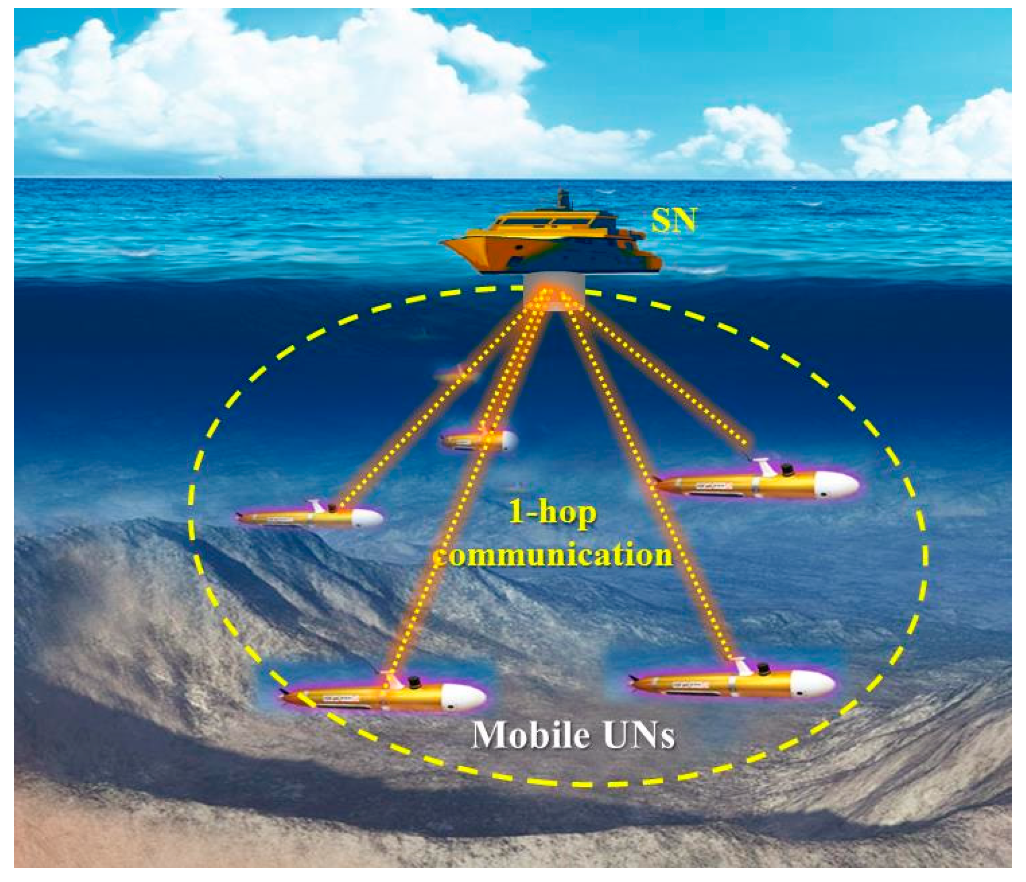
Figure 2.
Flow chart for the initialization phase of the APD-TDMA.
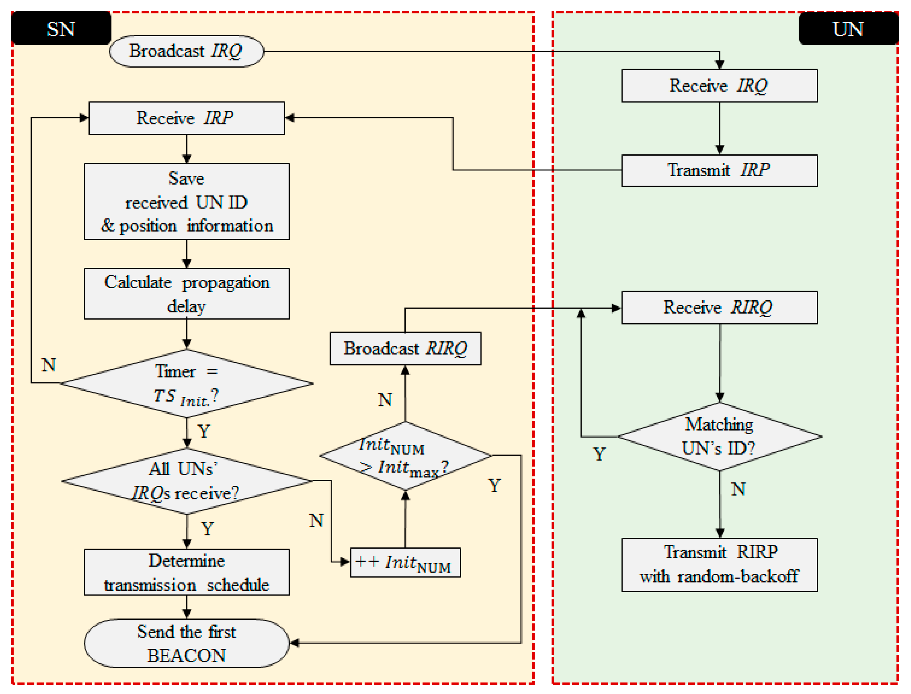
Figure 3.
APD-TDMA with three UNs.

Figure 4.
The transmission phase of the APD-TDMA.

Figure 5.
Flow chart for the transmission scheduling algorithm of the APD-TDMA.
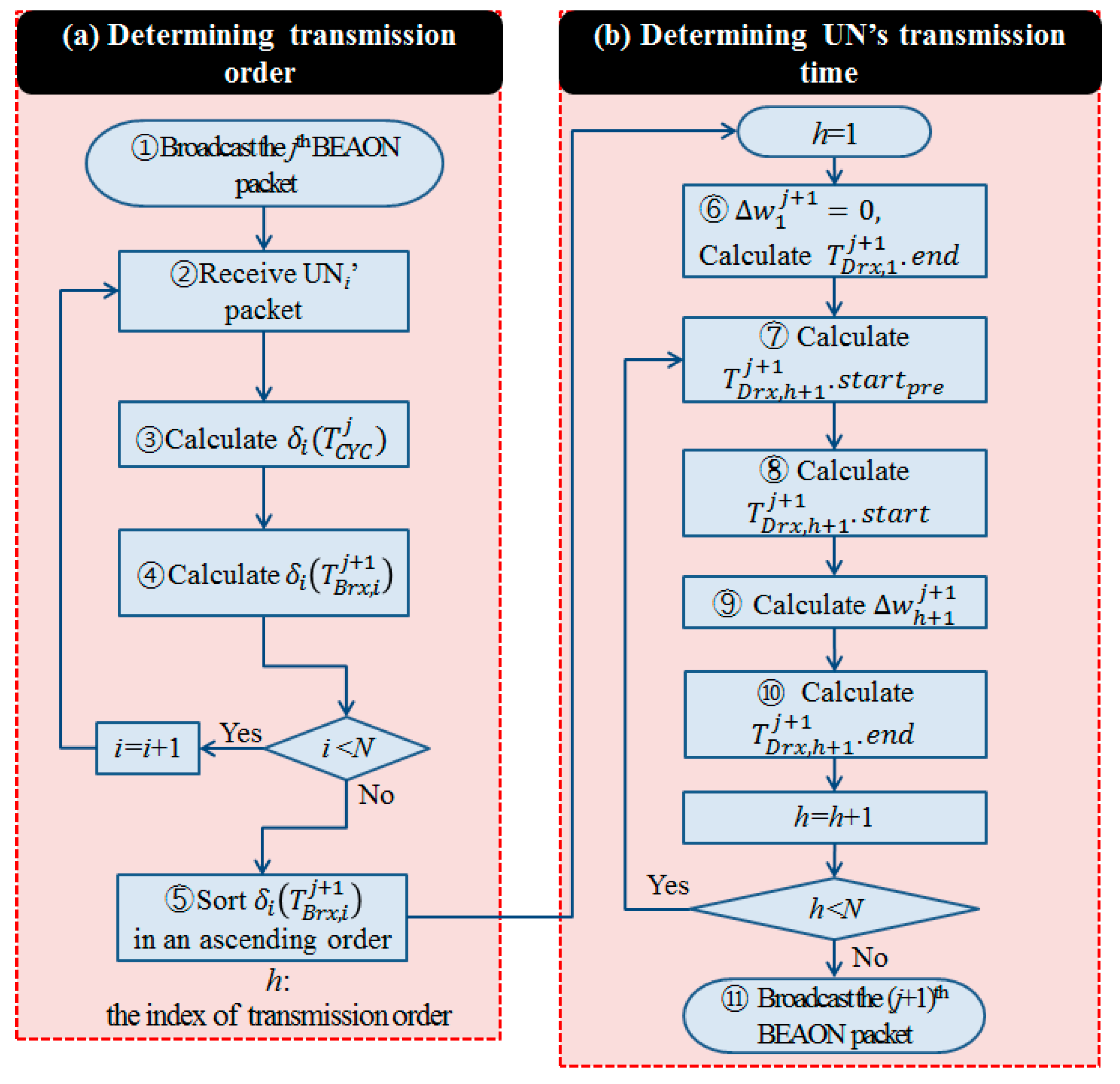
Figure 6.
Performance degradation by the transmission order in which 10 nodes move at the maximum speed of 7 m/s.
Figure 6.
Performance degradation by the transmission order in which 10 nodes move at the maximum speed of 7 m/s.
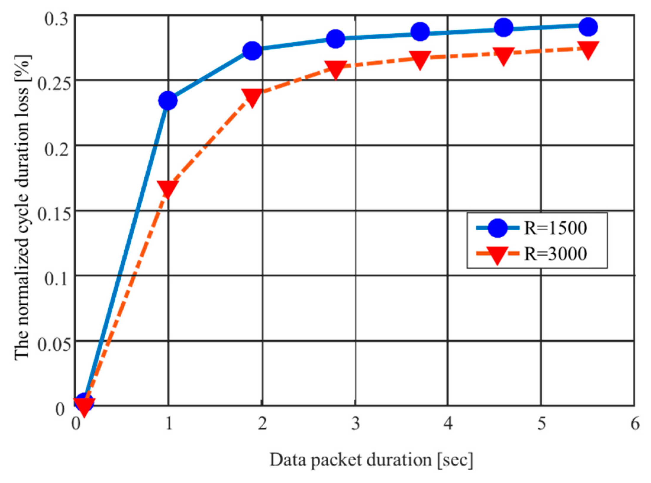
Figure 7.
Performances of the BTB-TDMA1 and the BTB-TDMA2 versus the length of a time block at 5 nodes, 25 nodes, and 50 nodes when the network range is 1500 m and the maximum speed of nodes is 5 m/s. (a) The CR of the BTB-TDMA1; (b) the CD of the BTB-TDMA1 and the BTB-TDMA2; (c) the CU of the BTB-TDMA1 and the BTB-TDMA2.
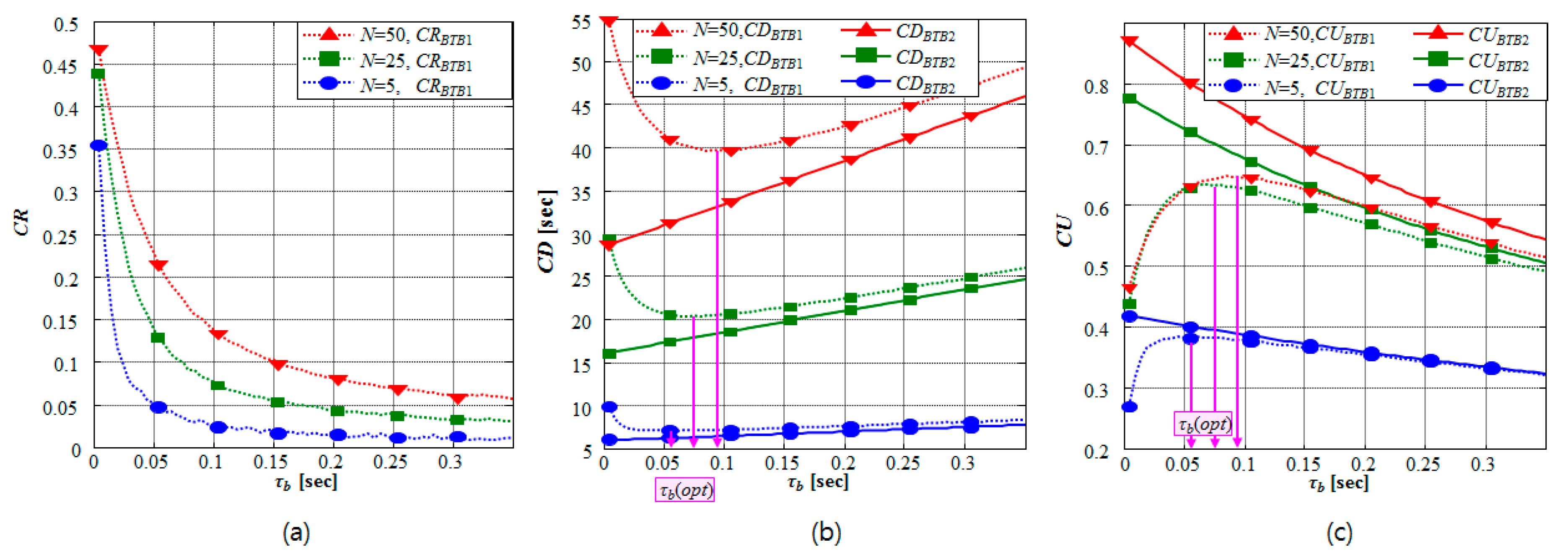
Figure 8.
(a) The CD and (b) the CU of the APD-TDMA and the BTB-TDMA versus the number of nodes in which the network range is 1500 m and the maximum speed of nodes is 5 m/s.
Figure 8.
(a) The CD and (b) the CU of the APD-TDMA and the BTB-TDMA versus the number of nodes in which the network range is 1500 m and the maximum speed of nodes is 5 m/s.

Figure 9.
(a) The CD and (b) the CU of the APD-TDMA and the BTB-TDMA versus the network range when 25 nodes move at the maximum speed of 5 m/s.
Figure 9.
(a) The CD and (b) the CU of the APD-TDMA and the BTB-TDMA versus the network range when 25 nodes move at the maximum speed of 5 m/s.
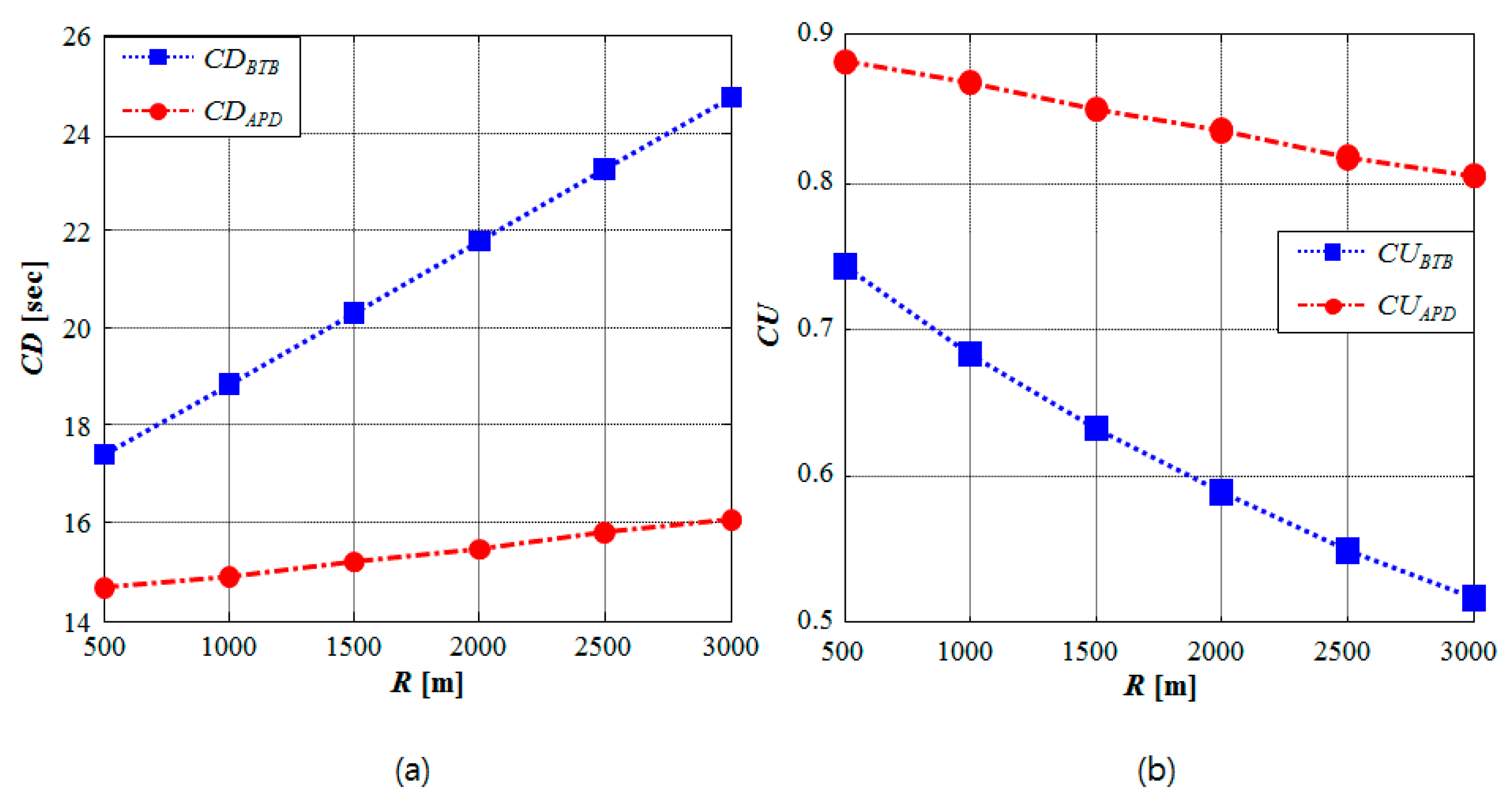
Figure 10.
(a) The CD and (b) the CU of the APD-TDMA and the BTB-TDMA versus the maximum speed of nodes when the number of nodes is 25 and the network range is 1500 m.
Figure 10.
(a) The CD and (b) the CU of the APD-TDMA and the BTB-TDMA versus the maximum speed of nodes when the number of nodes is 25 and the network range is 1500 m.

© 2018 by the authors. Licensee MDPI, Basel, Switzerland. This article is an open access article distributed under the terms and conditions of the Creative Commons Attribution (CC BY) license (http://creativecommons.org/licenses/by/4.0/).
Share and Cite
MDPI and ACS Style
Cho, A.-R.; Yun, C.; Lim, Y.-K.; Choi, Y. Asymmetric Propagation Delay-Aware TDMA MAC Protocol for Mobile Underwater Acoustic Sensor Networks. Appl. Sci. 2018, 8, 962. https://doi.org/10.3390/app8060962
AMA Style
Cho A-R, Yun C, Lim Y-K, Choi Y. Asymmetric Propagation Delay-Aware TDMA MAC Protocol for Mobile Underwater Acoustic Sensor Networks. Applied Sciences. 2018; 8(6):962. https://doi.org/10.3390/app8060962
Chicago/Turabian StyleCho, A-Ra, Changho Yun, Yong-Kon Lim, and Youngchol Choi. 2018. "Asymmetric Propagation Delay-Aware TDMA MAC Protocol for Mobile Underwater Acoustic Sensor Networks" Applied Sciences 8, no. 6: 962. https://doi.org/10.3390/app8060962
Note that from the first issue of 2016, this journal uses article numbers instead of page numbers. See further details here.