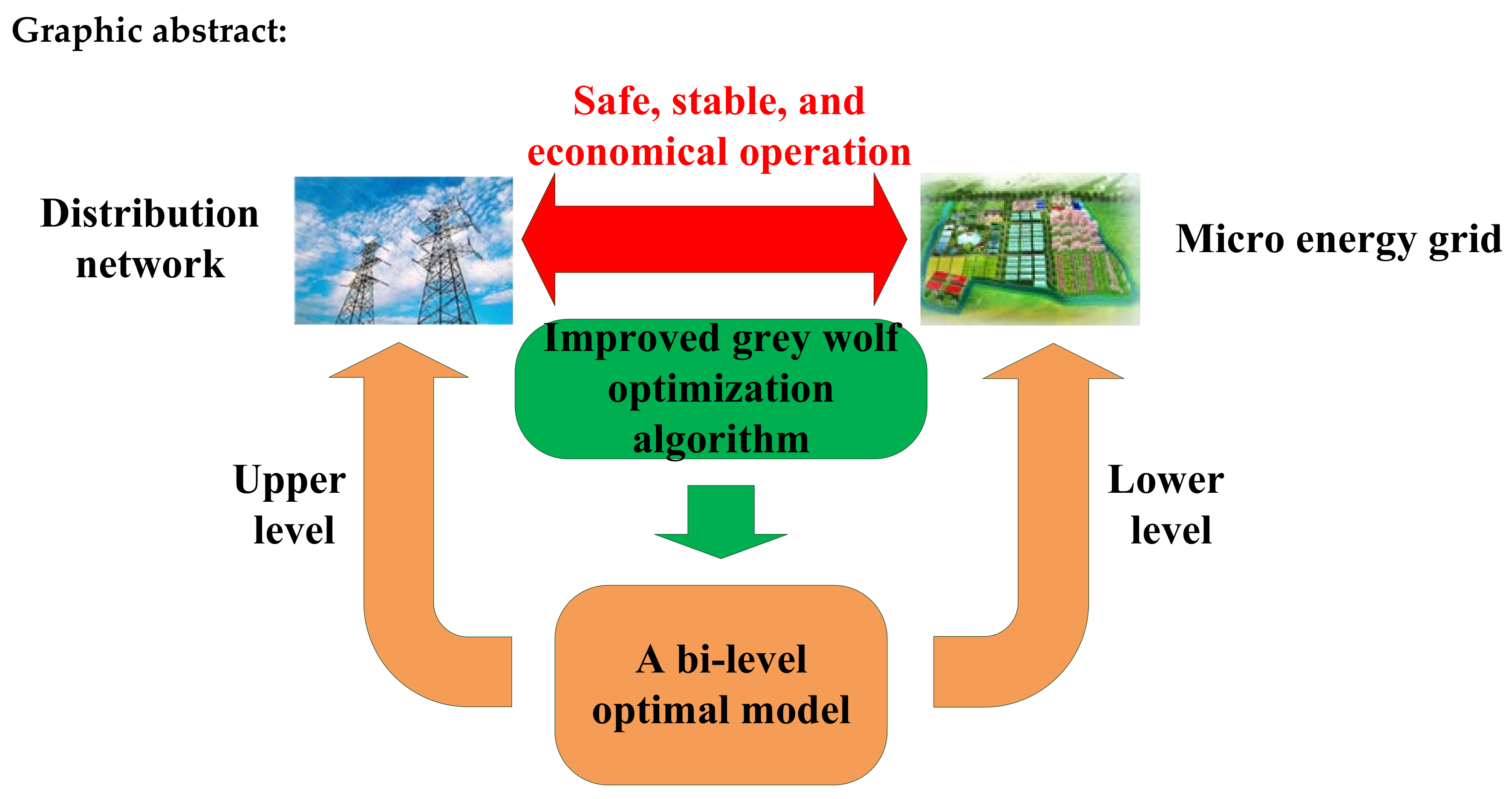
Optimal Operation Analysis of the Distribution Network Comprising a Micro Energy Grid Based on an Improved Grey Wolf Optimization Algorithm

Featured Application

A bi-level optimal model and relevant algorithm is proposed in the paper to achieve the safe, stable, and economical operation of the distribution network comprising a micro energy grid. The model and algorithm proposed in the paper can provide useful theoretical reference for the integrated energy service company to achieve optimal operation and control of the distribution network comprising a micro energy grid.

Abstract

With a focus on the safe, stable, and economical operation of a micro energy grid and a distribution network, this study proposes a bi-level optimal model for the integrated operation of a micro energy grid and a distribution network. The upper model used the minima of three objectives, including the integrated operating cost of the distribution network, the network’s active power loss, and the standard deviation of the voltage deviation in the distribution network. The lower model used the minimum integrated operating cost for the micro energy grid as the objective function. Considering the large number of objectives in the upper model, and that no single optimal solution existed, the judgment-matrix method was used to obtain the weight factors of each objective, and the upper multi-objective optimization problem was transformed into a single-objective problem in this paper. A grey wolf optimization algorithm based on the dynamic adjustment of the proportional weight and convergence factor was proposed to solve the operating model of the distribution network comprising the micro energy grid. This algorithm offers a high solution precision, a high convergence speed, and a strong global searching ability. The nonlinear convergent factor formula proposed in this paper dynamically adjusted the global searching ability of the algorithm, while the proposed proportional weight sped up the convergence of the algorithm. The superiority of the proposed algorithm was verified mathematically by six test functions. The simulation results demonstrated that the model and algorithm proposed in this paper improved the economic benefits, and voltage stability of the distribution network, reduced the active power loss of the distribution network, and enabled the safe, stable, and economical operation of the distribution network comprising a micro energy grid.

1. Introduction

With the increased level of integration in the fields of energy, automation, computers, and communications, the micro energy grid attracted the attention of an increasing number of experts and scholars [1,2,3], who integrated them into electricity, heating, cooling, and gas grids. The micro energy grid is a micro integrated energy system [4,5,6], and a natural extension of the microgrid, which is mainly used in urban communities, industrial and agricultural parks, and rural areas. The micro energy grid is a user-side energy interconnection. By means of information, the power-supply grids for cooling, heating, electricity, and gas in the micro energy grid are coordinated for optimization, in an effort to meet the demands for various energies on the user side, and to achieve comprehensive and efficient utilization of various energies. Photovoltaic (PV) power, wind power, microturbines, and other distributed energies in the form of a micro energy grid accessing a distribution network are becoming increasingly widespread [7]. The micro energy grid is the link between distribution networks and distributed energy, such that the distribution network does not have to manage distributed energies of various types, large quantities, or decentralized access (especially intermittent). Based on the above advantages, many demonstration projects, such as the new Tianjin Eco-city [7], the Golden Concord Group Limited (GCL) Suzhou Industrial Park multi-complementary model [8], and the ”Forest Town” of Jurong [9], exist in China. Therefore, the coordination of the operation of the distribution network and the micro energy grid, so as to maximize the consumption and utilization of renewable energy, and improve the operating economy, security, and stability of the entire system, is an urgent problem requiring resolution by researchers.

Numerous studies in China and abroad focused on the optimal dispatching of the distributed energy’s direct access to the distribution network [10,11,12,13,14,15,16,17,18,19]. For example, in Reference [12], a distributed coordinated control framework for a distribution network was proposed to enable reactive power optimization of the distribution network with renewable energy, and to improve the power quality of the system. In Reference [13], an optimal dispatching method for an active distribution network considering the risk of voltage instability was proposed. In Reference [15], a comprehensive optimization algorithm for a distribution network was proposed to enable the simultaneous optimization of renewable energy output, distribution network reconfiguration, and capacitor switching. According to the research reported in the above references, the control variables of the system will feature an increasing amount of distributed renewable energy in the distribution network, which complicates the solution process, and is disadvantageous to the solution of the model. As a result of the continuous development of microgrid technology [20,21,22,23], experts and scholars in China and abroad studied the optimal dispatching problem of renewable energy in the form of microgrid access to a distribution network [24,25,26,27,28]. For example, Reference [27] considered the various interest demands of the microgrid and the distribution network, established a game relationship model of the two, proposed a cooperative evolutionary game algorithm to solve the above model, and achieved coordinated operation of the microgrid and the distribution network. However, the above studies were based on research on a single electrical energy. Typical situations were not fully considered, such as the dispatching of a micro energy grid comprising cooling, heating, electricity, and gas, and the coordination of the operation of the micro energy grid and the distribution network when the micro energy grid is accessible by the distribution network.

For the solution of a dispatching model, the interior point method and other non-intelligent algorithms may not be able to achieve an optimal solution when a large amount of computation is required. The particle swarm optimization (PSO) algorithm converged early, and often provided a local optimal solution [29]. Some references proposed the grey wolf optimization (GWO) algorithm [30,31,32], which was reported to show a better convergence rate and optimization ability when compared with the PSO algorithm. For example, Reference [31] proposed a method to solve the cogeneration dispatching model using the GWO algorithm, and achieved economical operation of the cogeneration system. Reference [32] proposed an innovative tuning approach for fuzzy control systems, with reduced parametric sensitivity using the GWO algorithm. However, some deficiencies existed in the convergence speed and global optimization ability of the above algorithms.

In summary, the current research had the following problems: (1) In the distribution network comprising the microgrid, only a simple electrical-load demand existed, and the demands of heating and cooling loads were not considered. (2) Recent studies of the interaction between the microgrid and the distribution network considered only the economic performance of both sides, and did not consider that the output power of the microgrid would affect the operation of the distribution network. In fact, the output power of the microgrid will affect the stability and security of the operation of the distribution network, and the dispatching demand of the distribution network for the microgrid will also affect the economy of the microgrid; therefore, optimal operation of both sides involves mutual restraint and mutual influence.

To address the above problems, the contributions of this paper are presented as follows:

(1) The power-supply structure of a micro energy grid comprising cooling, heating, electricity, and gas grids was established. The energies of cooling, heating, electricity, and gas transformed and supported each other. Then, the operation structure of a distribution network comprising the micro energy grid was established. At the same time, the demands of the heating, cooling, and electricity loads were comprehensively considered.

(2) Considering the interaction between the micro energy grid and the distribution network, a bi-level optimal model for their integrated operation was proposed. The upper model used the minima of three objectives, including the integrated operating cost of the distribution network, the network’s active power loss, and the standard deviation of the voltage deviation in the distribution network. The lower model used the minimum integrated operating cost for the micro energy grid as the objective function.

(3) A grey wolf optimization algorithm based on the dynamic adjustment of the proportional weight and convergence factor was proposed to solve the model, which overcame the problem of the local optimum and slow convergence rate associated with the traditional particle swarm algorithm, and the grey wolf algorithm. Then, the superiority of the proposed algorithm was verified mathematically by six test functions.

(4) China’s Gansu region is rich in wind and solar energy resources. To fully exploit these resources, a demonstration project of the micro energy grid in an agricultural park is being established. The safe, stable, and economical operation of the distribution network and the micro energy grid will be addressed in the future. Therefore, the model and algorithm were analyzed in an actual 10-kV distribution network in a region of Gansu Province, China.

The organization of the remainder of this paper is as follows: Section 2 establishes the operation structure of the distribution network comprising the micro energy grid, according to the problems discussed. Section 3 establishes a bi-level optimal model for the integrated operation of the micro energy grid and the distribution network. Section 4 proposes a grey wolf optimization algorithm, based on the dynamic adjustment of the proportional weight and convergence factor, to solve the model. Section 5 uses a case study in an actual 10-kV distribution network in a region of Gansu Province, China to demonstrate the validity of the proposed model and method. The full paper is summarized and future work is described in Section 6. The general workflow for the optimal operation of the distribution network comprising the micro energy grid, based on the improved grey wolf optimization algorithm, is shown in Figure 1.

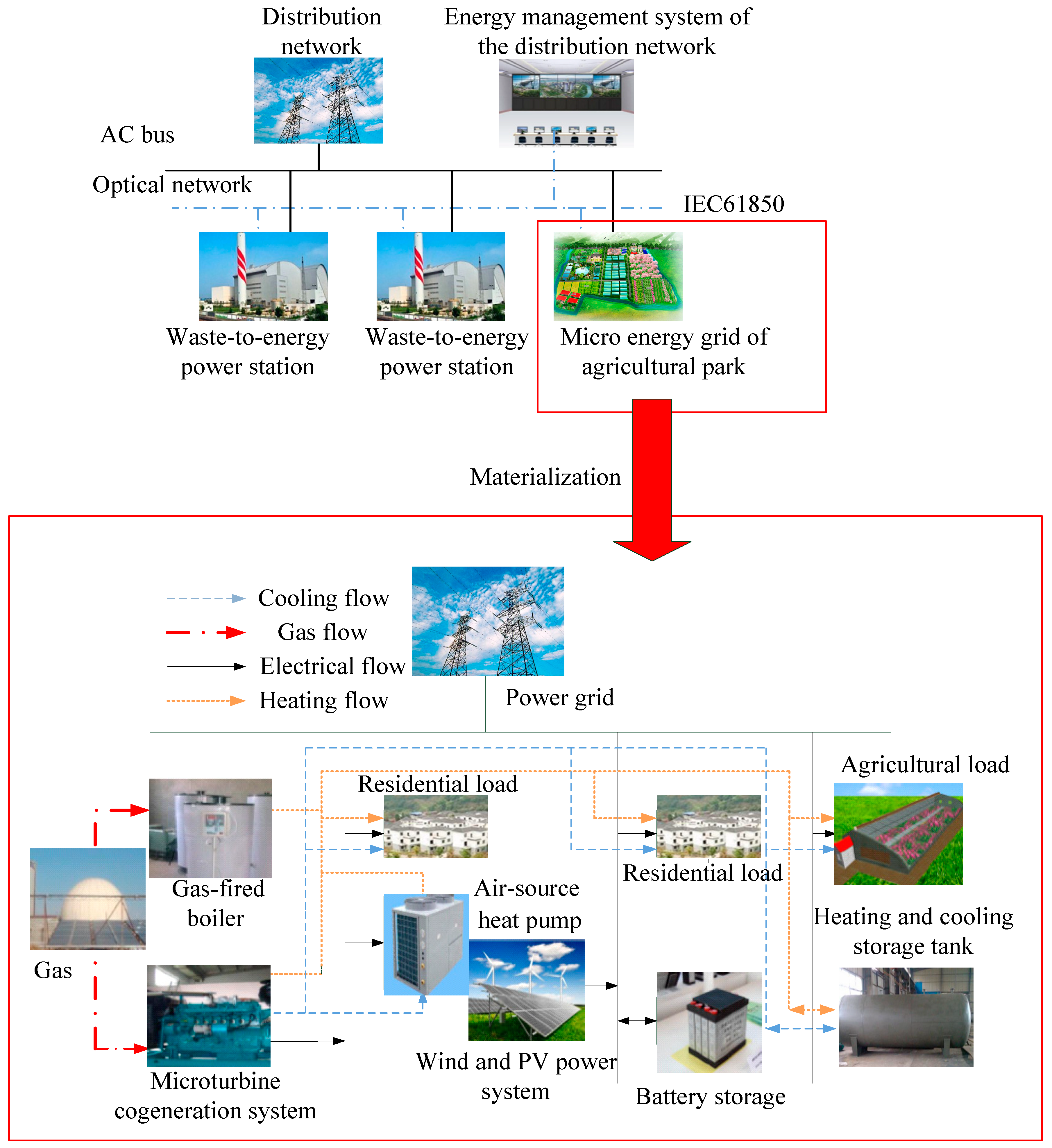
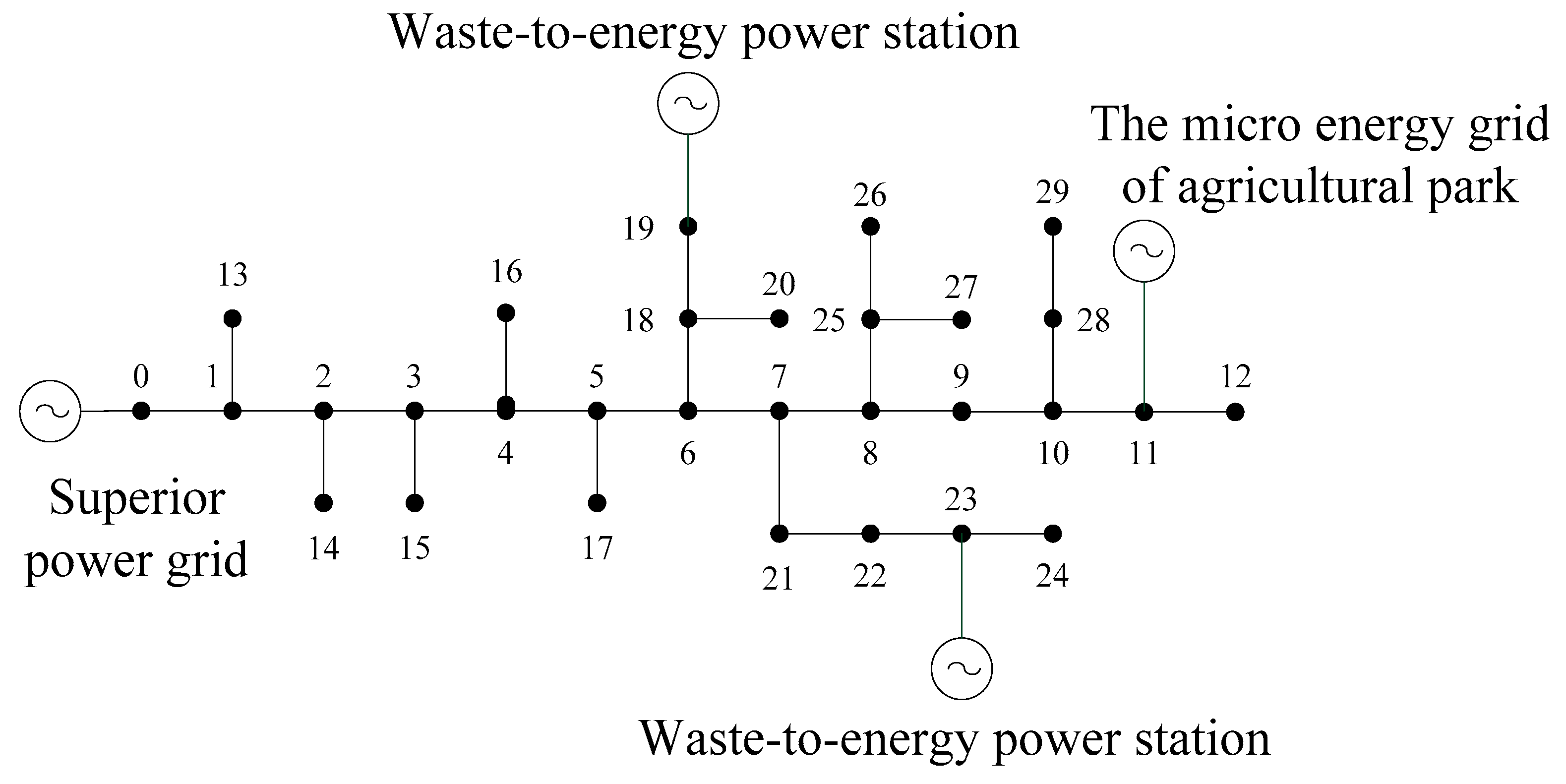
2. Operating Structure of a Distribution Network Comprising a Micro Energy Grid

The operating structure of a distribution network comprising a micro energy grid is shown in Figure 2. The energy management module of the distribution network was the “brain”, and was the key component of the optimal distribution-network operation. The micro energy grid and waste-to-energy power station connected to each node were managed by the distribution-network energy-management module. As the lower level of the distribution network, the micro energy grid provided the necessary electrical measurement data for the distribution network, and provided decision support for the dispatch of the distribution network. The communication network between the upper and lower levels was an optical network, and the communication protocol was IEC61850 (International Electrotechnical Commission) [33]. The micro energy grid included PV power, wind power, microturbines, gas-fired boilers, heat-recovery boilers, lithium-bromide absorption-type refrigerators, battery storage, heating and cooling storage tanks, and air-source heat pumps. The micro energy grid was connected to a node of the distribution network. PV power, wind power, and microturbines were used to satisfy the internal electrical load of the micro energy grid. Heat-recovery boilers, lithium-bromide absorption-type refrigerators, and air-source heat pumps were used to satisfy the internal heating load of the micro energy grid. Battery storage, and heating and cooling storage tanks mainly had roles in the adjustment of the micro energy grid. The energies of cooling, heating, electricity, and gas transformed and supported each other, thus improving the efficiency of the comprehensive energy utilization.

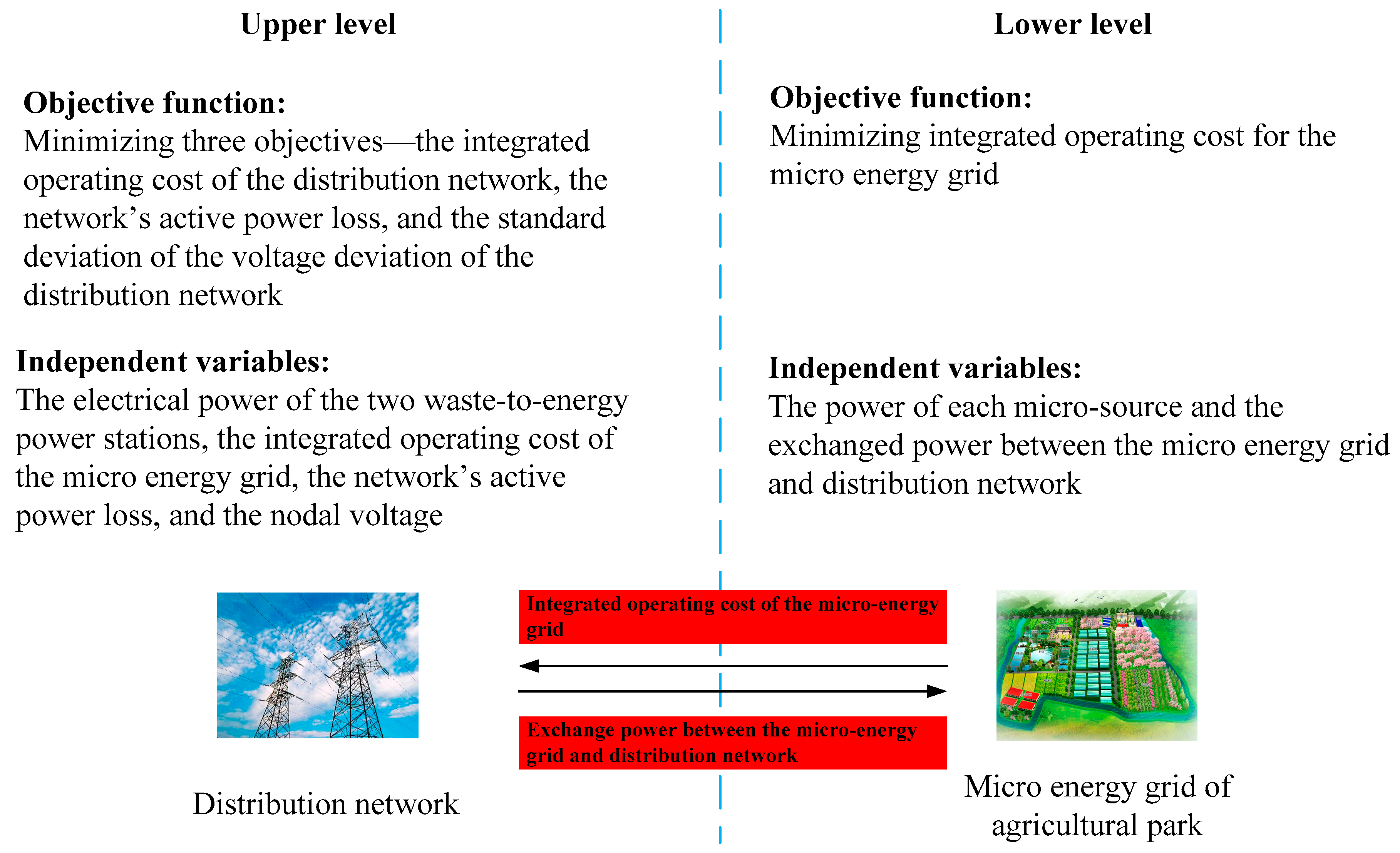
3. Bi-Level Optimal Model of a Distribution Network Comprising a Micro Energy Grid

The power-supply structure of the micro energy grid and the distribution network were established in the previous section. Based on that structure, a bi-level optimal dispatching model of a distribution network with a micro energy grid was established. The upper level was the distribution network, and the lower level was the micro energy grid. The upper model used the minima of three objectives—the integrated operating cost of the distribution network, the network’s active power loss, and the standard deviation of the voltage deviation in the distribution network. The lower model used the minimum integrated operating cost for the micro energy grid as the objective function. The exchanged power between the micro energy grid and the distribution network was set to the optimized output of the upper level, which was regarded as a known quantity in the lower optimization model. The integrated operating cost for the micro energy grid was set to the optimized output of the lower level, which was regarded as a known quantity in the upper optimization model. The upper model was optimized according to the optimal result of the lower level, and repeated until the optimal solution was achieved. The dispatching period was 24 h. The bi-level optimization model is shown in Figure 3.

3.1. Optimal Model of the Distribution Network

3.1.1. Objective Function

The power-supply equipment connected to the upper distribution network mainly included two waste-to-energy power stations, and the micro energy grid. The upper model used the minima of three objectives—the integrated operating cost of the distribution network, the network’s active power loss, and the standard deviation of the voltage deviation in the distribution network. Because the number of objectives in the distribution-network level was large, the judgment-matrix method [34] was used to transform the multi-objective problem into a single-objective problem in this research. The weight vector was $W=(0.5393,0.2974,0.1633)$. The independent variables of the function were the electrical power of the two waste-to-energy power stations, the integrated operating cost of the micro energy grid, the network’s active power loss, and the nodal voltage. In this paper, the costs of the distribution line, transformer, and switchgear mainly considered the overall cost of periodical inspection, cleaning, and annual preventive experiments, which was set as a fixed cost and was not embodied in the objective function. The objective function was defined as follows:

$$F_1=\min [w_1{F}_2(t)+w_2{F}_3(t)+w_3{F}_4(t)].$$

(1)

$$\{\begin{array}{l}{F}_2(t)={\displaystyle \sum _{t=1}^T}[C_{\mathrm{gp}1}{P}_{\mathrm{gp}1}(t)+C_{\mathrm{gp}2}{P}_{\mathrm{gp}2}(t)+F_5(t)]\\ F_3(t)={\displaystyle \sum _{t=1}^T{P}_{\mathrm{loss}}(t)}\\ F_4(t)={\displaystyle \sum _{t=1}^T\sqrt{\frac{1}{N}{\displaystyle \sum _{i=1}^N{(\Delta U_i(t))}^2}})={\displaystyle \sum _{t=1}^T\sqrt{\frac{1}{N}{\displaystyle \sum _{i=1}^N{(U_i(t)-U_R)}^2}})}}\end{array},$$

(2)

where $F_2(t)$ is the integrated operating cost of the distribution network; $F_3(t)$ is the active power loss of the distribution network; $F_4(t)$ is the standard deviation of the voltage deviation in the distribution network, which was used to measure the voltage deviation in the distribution network in a dispatching cycle; $F_5(t)$ is the integrated operating cost of the micro energy grid; $C_{\mathrm{gp}}$ is the cost of garbage power; $P_{\mathrm{gp}}(t)$ is the electrical power of garbage power; $P_{\mathrm{loss}}(t)$ is the active power loss of the distribution network; $\Delta U_i(t)$ is the voltage deviation in the distribution network; $U_i(t)$ is the voltage of node $i$; $U_{\mathrm{R}}$ is the rated value of the nodal voltage; $N$ is the number of nodes in the distribution network; and $T$ is the dispatching cycle.

3.1.2. Constraint Conditions

(1) Constraints for the balance of the electrical power

$$P_{\mathrm{gp}1}(t)+P_{\mathrm{gp}2}(t)+P_{\mathrm{exgrid}}(t)=P_{\mathrm{load}}(t)+P_{\mathrm{loss}}(t),$$

(3)

where $P_{\mathrm{load}}(t)$ is the electrical load, and $P_{\mathrm{exgrid}}^{}(t)$ is the exchanged electrical power between the micro energy grid and the distribution network.

(2) Constraints for the load flow equations

$$\{\begin{array}{l}{P}_i=U_i{\displaystyle \sum _{j=1}^N{U}_j(G_{ij}^{}\cos {\theta }_{ij}+B_{ij}\sin {\theta }_{ij})}\\ Q_i=U_i{\displaystyle \sum _{j=1}^N{U}_j(G_{ij}^{}\cos {\theta }_{ij}-B_{ij}\sin {\theta }_{ij})}\end{array},$$

(4)

where $P_i$ is the injected active power of node $i$; $Q_i$ is the injected reactive power of node $i$; $U_i$ and $U_j$ are the voltage magnitudes of nodes $i$ and $j$, respectively; $G_{ij}^{}$ is the conductivity between nodes $i$ and $j$; $B_{ij}$ is the electrical susceptance; and ${\theta }_{ij}$ is the phase difference between nodes $i$ and $j$.

(3) Constraints for the electrical power of garbage power

$$\{\begin{array}{l}{P}_{\mathrm{gp}1}^{\min }\le P_{\mathrm{gp}1}(t)\le P_{\mathrm{gp}1}^{\max }\\ P_{\mathrm{gp}2}^{\min }\le P_{\mathrm{gp}2}(t)\le P_{\mathrm{gp}2}^{\max }\end{array},$$

(5)

where $P_{\mathrm{gp}}^{\min }$ and $P_{\mathrm{gp}}^{\max }$ are the minimum and maximum electrical powers of garbage power, respectively.

(4) Constraints for the nodal voltage

$$U_i^{\min }\le U_i(t)\le U_i^{\max },$$

(6)

where $U_i^{\min }$ and $U_i^{\max }$ are the minimum and the maximum values of nodal voltage, respectively.

(5) Constraints for the voltage deviation

According to the GB12325-2008-T allowable deviation of power-quality supply voltage, the voltage deviation was expressed as the following:

$$\Delta U_i(t)=U_i(t)-U_{\mathrm{R}},U_i\le 0.93U_{\mathrm{R}}or{U}_i\ge 1.07U_{\mathrm{R}}.$$

(7)

3.1.3. Processing Method for Transforming the Multi-Objective Model into a Single-Objective Model

A multi-objective problem cannot be visually compared with data values; instead, it must be transformed into a single-objective function. The judgment matrix is a method for the quantitative and qualitative calculation of weights that reflect the objective situation to a certain extent, and consider the importance of different users to each objective. In this paper, the judgment-matrix method [34] was used to transform the multi-objective function into a single-objective function. The original multi-objective function was transformed into the following:

$$F_1=\min (B_1{F}_2{}^{\prime }(t)+B_2{F}_3{}^{\prime }(t)+B_3{F}_4{}^{\prime }(t)]),$$

(8)

where $F_2{}^{\prime }(t)$, $F_3{}^{\prime }(t)$, and $F_4{}^{\prime }(t)$ are the normalized values of the objective function (i.e., transformed into the range [0, 1]). $B_1$, $B_2$, and $B_3$ are the weight factors. The different dimensions of the objective function were eliminated based on the effect of the optimal result.

The main goal of the judgment-matrix method was to determine the judgment matrix according to the hierarchical relationship between the goals. The criteria were formed as shown in

Table 1. Formation criteria of the judgment matrix.

Scale	Meaning
1	Comparing two factors, they are equally important.
3	Comparing two factors, one is slightly more important than the other.
5	Comparing two factors, one is more important than the other.
7	Comparing two factors, one is significantly more important than the other.
9	Comparing two factors, one is strongly more important than the other.
2, 4, 6, 8	The scale of compromise between two adjacent judgments.

Note: When comparing factors $i$ and $j$, the judging result is $x_{ij}$, whereas the judging result is $x_{ji}=\frac{1}{x_{ij}}$ when comparing factors $j$ and $i$.

.

According to the problems outlined in this study, the goals were graded by importance. The importance of each index was judged by expert experience. According to the actual circumstances of distribution networks in China, the power-supply voltage quality can meet the national standard; therefore, reducing the operating cost is the primary concern of power enterprises. In this paper, the integrated operating cost of the distribution network was the first grade goal. The standard deviation of the voltage deviation in the distribution network was the second grade goal. The network’s active power loss was the third grade goal. Combined with the above analysis, the judgment matrix was formed as follows:

$$J=\left[\begin{array}{ccc}1& 2& 3\\ 1/2& 1& 2\\ 1/3& 1/2& 1\end{array}\right].$$

(9)

After matrix processing, the weight vector of the objective function was determined to be $W=(0.5393,0.2974,0.1633)$.

3.2. Optimal Micro-Energy-Grid Model

3.2.1. Objective Function

The power-supply equipment of the lower micro energy grid mainly included PV power, wind power, microturbines, gas-fired boilers, heat-recovery boilers, lithium-bromide absorption-type refrigerators, battery storage, heating and cooling storage tanks, and air-source heat pumps. The lower model used the minimum integrated operating cost for the micro energy grid as the objective function. The integrated operating costs of the micro energy grid included the cost of equipment maintenance, the cost of the exchanged electrical power between the distribution network and the micro energy grid, the cost of environmental pollution, the cost of fuel, and the cost of investment depreciation in a dispatching cycle. The independent variables of the function were the power of each micro-source, and the exchanged power between the micro energy grid and the distribution network. In the micro energy grid, the cost of line maintenance was set to a fixed cost, and was not reflected in the objective function. The objective function is shown below.

$$\begin{array}{l}\min F_5(t)=\min [{\displaystyle \sum _{t=1}^{24}(\frac{Z_1(t)+Z_2(t)}{2}\left|P_{\mathrm{exgrid}}(t)\right|+\frac{Z_1(t)-Z_2(t)}{2}\left|P_{\mathrm{exgrid}}(t)\right|}+\\ {\displaystyle \sum _{x=1}^n(C_x(t)+E_x\frac{l{(1+l)}^{A_x}}{{(1+l)}^{A_x}-1})P_x(t)}+{\displaystyle \sum _{x=1}^n{C}_{\mathrm{fuel}x}{P}_x(t)}+{\displaystyle \sum _{x=1}^n{\displaystyle \sum _{y=1}^m((C_y+D_y)B_{xy}{P}_x(t))}})]\end{array},$$

(10)

where $C_x(t)$ is the cost of equipment maintenance of micro-source x; $C_{\mathrm{fuel}x}$ is the cost of fuel of micro-source x; $E_x$ is the cost of initial fixed investment of micro-source x; $l$ is the interest rate; $A_x$ is the lifespan of micro-source x; $P_x(t)$ is the electrical power of micro-source x; $C_y$ is the penalty of pollutant gas y; $D_y$ is the environmental value of pollutant gas y; and $B_{xy}$ is the value of pollutant gas y, which is produced by micro-source x. $Z_1(t)$ is the price of purchasing electricity for the micro energy grid. $Z_2(t)$ is the price of selling electricity for the micro energy grid.

3.2.2. Constraint Conditions

(1) Constraints for the cooling-heating-electrical power balance of the micro energy grid

$$\{\begin{array}{l}{P}_{\mathrm{CASHP}}^{}(t)+P_{\mathrm{AC}}^{}(t)+P_{\mathrm{cstor}}^{}(t)=P_{\mathrm{coolingload}}^{}(t)\\ P_{\mathrm{HASHP}}^{}(t)+P_{\mathrm{EB}}^{}(t)+P_{\mathrm{GB}}^{}(t)+P_{\mathrm{hstor}}^{}(t)=P_{\mathrm{heatload}}^{}(t)\\ P_{\mathrm{estor}}^{}(t)+P_{\mathrm{MT}}^{}(t)+P_{\mathrm{exgrid}}^{}(t)+P_{\mathrm{WT}}^{}(t)+P_{\mathrm{PV}}^{}(t)=P_{\mathrm{electriload}}^{}\left(\mathrm{t}\right)+P_{\mathrm{ASHP}}^{}(t)\end{array},$$

(11)

where $P_{\mathrm{CASHP}}^{}(t)$ is the exchanged cooling power of the air-source heat pump; $P_{\mathrm{AC}}^{}(t)$ is the cooling power of the lithium-bromide absorption-type refrigerator; $P_{\mathrm{cstor}}^{}(t)$ is the charging or discharging cooling power of the cooling storage tank (the value of discharging cooling power is negative, and the value of charging cooling power is positive); $P_{\mathrm{coolingload}}^{}(t)$ is the cooling load; $P_{\mathrm{HASHP}}^{}(t)$ is the exchanged heating power of the air-source heat pump; $P_{\mathrm{EB}}^{}(t)$ is the heating power of the heat-recovery boiler; $P_{\mathrm{GB}}^{}(t)$ is the heating power of the gas-fired boiler; $P_{\mathrm{hstor}}^{}(t)$ is the charging or discharging heating power of the heating storage tank (the value of discharging heating power is negative, and the value of charging heating power is positive); $P_{\mathrm{heatload}}^{}(t)$ is the heating load; $P_{\mathrm{estor}}^{}(t)$ is the charging or discharging electrical power of the battery storage (the value of discharging electrical power is negative, and the value of charging electrical power is positive); $P_{\mathrm{MT}}^{}(t)$ is the electrical power of the microturbine; $P_{\mathrm{WT}}^{}(t)$ is the electrical power of wind power; $P_{\mathrm{PV}}^{}(t)$ is the electrical power of PV; $P_{\mathrm{ASHP}}^{}(t)$ is the electrical power of the air-source heat pump in exchanging cooling or heating power; and $P_{\mathrm{electriload}}^{}\left(\mathrm{t}\right)$ is the electrical load.

(2) Constraints for battery storage, and the cooling and heating storage tanks

Battery storage, and heating and cooling storage tanks played the role of peak load shifting in the micro energy grid. Their working principles were similar. Therefore, their general constraints were as follows:

$$E_{\min }\le E(\mathrm{t})\le E_{\max }.$$

(12)

$$E(0)=E(T).$$

(13)

$$P_{\mathrm{stor}}^t=\{\begin{array}{l}{P}_{\mathrm{dis}}^t,0\le P_{\mathrm{dis}}^t\le P_{\mathrm{dmax}},P_{\mathrm{stor}}^t\ge 0\\ -P_{\mathrm{ch}}^t,0\le P_{\mathrm{ch}}^t\le P_{\mathrm{cmax}},P_{\mathrm{stor}}^t<0\end{array},$$

(14)

where $E(\mathrm{t})$ is the capacity of battery storage, and the heating and cooling storage tanks at time t; $E_{\min }$ and $E_{\max }$ are the maximum and minimum capacities of battery storage, and the heating and cooling storage tanks, respectively; and $P_{\mathrm{cmax}}$ and $P_{\mathrm{dmax}}$ are the maximum charging and discharging powers of battery storage, and the heating and cooling storage tanks, respectively.

(3) Exchanged electrical power between the distribution network and the micro energy grid

$$P_{\mathrm{exgrid}}^{\min }\le P_{\mathrm{exgrid}}^{}(t)\le P_{\mathrm{exgrid}}^{\max },$$

(15)

where $P_{\mathrm{exgrid}}^{\min }$ and $P_{\mathrm{exgrid}}^{\max }$ are the minimum and maximum exchanged power between the distribution network and the micro energy grid, respectively.

(4) Ramping constraints

$$\{\begin{array}{l}-R_{\mathrm{MT}}^{\mathrm{down}}\le P_{\mathrm{MT}}^{}(t)-P_{\mathrm{MT}}^{}(t-1)\le R_{\mathrm{MT}}^{\mathrm{up}}\\ -R_{\mathrm{GB}}^{\mathrm{down}}\le P_{\mathrm{GB}}^{}(t)-P_{\mathrm{GB}}^{}(t-1)\le R_{\mathrm{GB}}^{\mathrm{up}}\end{array},$$

(16)

where $R_{\mathrm{MT}}^{\mathrm{down}}$ and $R_{\mathrm{MT}}^{\mathrm{up}}$ are the lower and upper ramp speeds of the microturbine, respectively; and $R_{\mathrm{GB}}^{\mathrm{down}}$ and $R_{\mathrm{GB}}^{\mathrm{up}}$ are the lower and upper ramp speeds of the gas-fired boiler, respectively.

(5) Constraints for each micro-source power limit

$$P_{\mathrm{every}}^{\min }\le P_{\mathrm{every}}^{}(t)\le P_{\mathrm{every}}^{\max },$$

(17)

where $P_{\mathrm{every}}^{}(t)$ is the cooling, heating, or electrical power of each micro-source in the micro energy grid; and $P_{\mathrm{every}}^{\min }$ and $P_{\mathrm{every}}^{\max }$ are the minimum and maximum cooling, heating, or electrical powers of each micro-source in the micro energy grid, respectively.

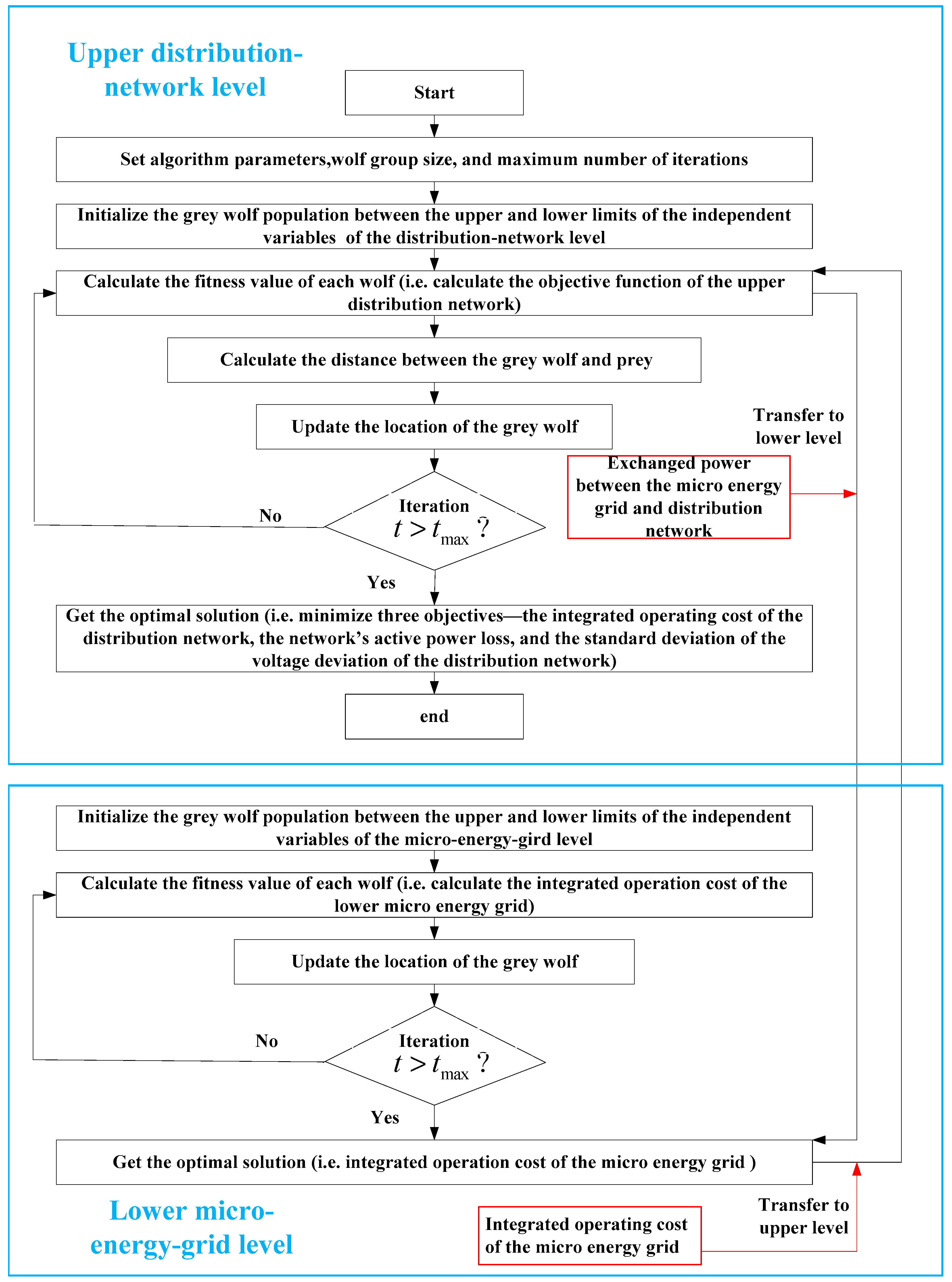
4. GWO Algorithm Based on the Dynamic Adjustment of the Proportional Weight and Convergence Factor

The problem solved for the operating model of the distribution network comprising the micro energy grid was a multivariate, nonlinear optimal problem with complex equations. The particle swarm optimization (PSO) algorithm converged early, and often provided a local optimal solution. Based on the above problem, the grey wolf optimization (GWO) algorithm based on the dynamic adjustment of the proportional weight and convergence factor was adopted to solve an optimal operating model in this study. This algorithm offers high solution precision, high convergence speed, and strong global searching ability.

4.1. Improved GWO Algorithm

The GWO algorithm is a new intelligent optimization algorithm proposed by Mirjalili in 2014. The GWO algorithm simulates the social hierarchy and predatory behavior of the grey wolf. The grey wolf is considered the predator at the top of the food chain. The GWO algorithm has the advantages of reduced parameter adjustment, simple principles, and ease of understanding. In the context of function optimization, the GWO algorithm surpasses the basic particle swarm algorithm in terms of accuracy and stability [30]. The search for the optimal solution is performed according to the three important steps in the hunting strategy of wolves: approaching, surrounding, and attacking prey. This process and the associated results were used to establish the model. Every grey wolf represented a potential solution in the population. The wolves were divided into four levels in the GWO algorithm: $\alpha$, $\beta$, $\delta$, and $\omega$. The current best individual was $\alpha$, which represented the optimal solution. The second- and third-best individuals were $\beta$ and $\delta$, respectively, which represented the suboptimal solution and third-best solution. The other individuals were recorded as $\omega$, which represented an ordinary solution. The corresponding hierarchical relationship was $\alpha >\beta >\delta >\omega$. A detailed description of the algorithm was provided in Reference [30].

However, the GWO algorithm also exhibits the problem of easily reaching a local optimal solution, as with any other swarm intelligence algorithm [35,36,37,38]. To address this problem, the GWO algorithm was improved in this study as follows:

(1) According to Reference [30], the value of $\overrightarrow{A}$ had a strong relationship with the local and global searches in the GWO algorithm. In Formula (19), $\overrightarrow{A}$ changes with the transformation of the convergence factor $\overrightarrow{a}$. The convergence factor $\overrightarrow{a}$ linearly decreases from 2 to 0 with continued iterations, easily resulting in a local optimal solution. In order to improve the global search abilities of the wolves, the improved nonlinear formula about the convergence factor $\overrightarrow{a}$ proposed in this study is shown in Formula (18). The original formulas of convergence factor $\overrightarrow{A},\overrightarrow{a}$ are shown in Formula (19).

$$\overrightarrow{a}=\overrightarrow{a_{\mathrm{ini}}}-(\overrightarrow{a_{\mathrm{ini}}}-\overrightarrow{a_{\mathrm{fin}}}+1){(\frac{t}{t_{\max }})}^2.$$

(18)

$$\{\begin{array}{l}\overrightarrow{A}=2\overrightarrow{a}\overrightarrow{r_2}-\overrightarrow{a}\\ \overrightarrow{a}=2-2(t/t_{\max })\end{array},$$

(19)

where $\overrightarrow{a_{\mathrm{ini}}}$ and $\overrightarrow{a_{\mathrm{fin}}}$ are the initial and final values, respectively, of convergence factor $\overrightarrow{a}$, with values of 2 and 0, respectively.

(2) In the later portion of the iterative process, loss of group diversity occurred because all grey wolves were close to the best individual region. If the current best individual grey wolf was the local optimal solution, then the GWO algorithm suffered from local optimization, resulting in premature convergence. Based on the PSO algorithm, a new proportional weight factor was introduced in this study. By adjusting the weight, the global search and local search abilities of the algorithm were balanced, and the convergence rate of the algorithm was improved. The proportional weight formulas were as follows:

$$\{\begin{array}{l}{w}_1=\frac{(\overrightarrow{A_1}\cdot \overrightarrow{K_1}){}^2\cdot \overrightarrow{{(X_1)}^2}}{\overrightarrow{(X_1^{}}{)}^2+\overrightarrow{{(X_2^{})}^2}+\overrightarrow{{(X_3^{})}^2}}\cdot \frac{1}{t_{\max }}\\ w_2=\frac{(\overrightarrow{A_2}\cdot \overrightarrow{K_2}){}^2\cdot \overrightarrow{{(X_2^{})}^2}}{\overrightarrow{(X_1^{}}{)}^2+\overrightarrow{{(X_2^{})}^2}+\overrightarrow{{(X_3^{})}^2}}\cdot \frac{1}{t_{\max }}\\ w_3=\frac{(\overrightarrow{A_3}\cdot \overrightarrow{K_3}){}^2\cdot \overrightarrow{{(X_3^{})}^2}}{\overrightarrow{(X_1^{}}{)}^2+\overrightarrow{{(X_2^{})}^2}+\overrightarrow{{(X_3^{})}^2}}\cdot \frac{1}{t_{\max }}\end{array}$$

(20)

$$\overrightarrow{X}(t+1)=\frac{(w_1{X}_1(\overrightarrow{t}+1)+w_2\overrightarrow{X_2}(t+1)+w_3\overrightarrow{X_3}(t+1))}{3},$$

(21)

where $w_1$, $w_2$, and $w_3$ are proportional weight factors; $\overrightarrow{A_1}$, $\overrightarrow{A_2}$, and $\overrightarrow{A_3}$ are convergence factors; and $\overrightarrow{K_1}$, $\overrightarrow{K_2}$, and $\overrightarrow{K_3}$ are swing factors.

The improved GWO algorithm was used to solve the dispatching model of the upper distribution network, and the lower micro energy grid in this study. The solving steps of the upper and lower models were similar. Therefore, the solving process for the dispatching model of the lower micro energy grid was used as an example. The solving steps were as follows:

(1) Initialize the population

$N$ was the size of the grey wolf population, and $n_2$ was the dimension of the grey wolf population (that is, the dimension of independent variables in the micro energy grid). The parameter $t_{\max }$ was the maximum number of iterations. The grey wolf population was randomly initialized between the upper and lower limits of the independent variables in the micro energy grid.

(2) Calculate the fitness value for each grey wolf

The fitness value of each grey wolf was calculated (that is, the integrated operating cost of the micro energy grid corresponding to the initial independent variables of each grey wolf). Then, the fitness values were compared. The optimal solution $\overrightarrow{X_{\alpha }}$, suboptimal solution $\overrightarrow{X_{\beta }}$, and third-best solution $\overrightarrow{X_{\delta }}$ of the initial independent variables of the grey wolves were determined.

(3) Calculate the distance between the grey wolf and the prey (that is, approach the prey)

When the grey wolves are hunting prey, they identify its position first. Then, they approach the prey. The formulas for this step were as follows:

$$\overrightarrow{D}=\left|\overrightarrow{K}\cdot \overrightarrow{X_{\mathrm{P}}}(t)-\overrightarrow{X}(t)\right|.$$

(22)

$$\overrightarrow{X}(t+1)={\overrightarrow{X}}_{\mathrm{p}}(t)-\overrightarrow{A}\cdot \overrightarrow{D}.$$

(23)

$$\{\begin{array}{l}\overrightarrow{K}=2\overrightarrow{r_1}\\ \overrightarrow{a}=\overrightarrow{a_{\mathrm{ini}}}-(\overrightarrow{a_{\mathrm{ini}}}-\overrightarrow{a_{\mathrm{fin}}}+1){(\frac{t}{t_{\max }})}^2\\ \overrightarrow{A}=2\overrightarrow{a}\overrightarrow{r_2}-\overrightarrow{a}\end{array},$$

(24)

where $\overrightarrow{D}$ is the distance between the grey wolf and the prey; $\overrightarrow{X_{\mathrm{p}}}(t)$ is the location of the prey at iteration $t$; $\overrightarrow{X}(t)$ is the location of the grey wolf at iteration $t$; $\overrightarrow{K}$ is the swing factor; $\overrightarrow{r_1}$ and $\overrightarrow{r_2}$ are random numbers between 0 and 1; $\overrightarrow{A}$ and $\overrightarrow{a}$ are convergence factors; $t$ is the current iteration; and $t_{\max }$ is the maximum number of iterations.

(4) Update the location of the grey wolf (that is, surround and attack the prey)

When the prey was surrounded, the grey wolves $\alpha$, $\beta$, and $\delta$ (the first three historical optimal locations of grey wolves $\overrightarrow{X_{\alpha }}$, $\overrightarrow{X_{\beta }}$, and $\overrightarrow{X_{\delta }}$, respectively) better understood the location of potential prey. Therefore, the best three individuals $\alpha$, $\beta$, and $\delta$ led other members to evaluate the location of the prey, so as to update their location. Finally, the grey wolves surrounded and attacked the prey (that is, identified an optimal solution of independent variables, and then obtained the optimal solution of the integrated operating cost of the micro energy grid). At this moment, the GWO algorithm completed an iteration. If $t<t_{\max }$, then the solving program returned to Step (2) for recalculation to obtain the optimal solution. If $t>t_{\max }$, then an optimal solution of the independent variables of an individual, and an objective function for the last iteration were shown. The formulas for this step were as follows:

$$\{\begin{array}{l}\overrightarrow{D_{\alpha }}=\left|\overrightarrow{K_1}\cdot \overrightarrow{X_{\alpha }}(t)-\overrightarrow{X}(t)\right|\\ \overrightarrow{D_{\beta }}=\left|\overrightarrow{K_2}\cdot \overrightarrow{X_{\beta }}(t)-\overrightarrow{X}(t)\right|\\ {\overrightarrow{D}}_{\delta }=\left|\overrightarrow{K_3}\cdot \overrightarrow{X_{\delta }}(t)-\overrightarrow{X}(t)\right|\end{array}.$$

(25)

$$\{\begin{array}{l}{w}_1=\frac{(\overrightarrow{A_1}\cdot \overrightarrow{K_1}){}^2\cdot \overrightarrow{{(X_1)}^2}}{\overrightarrow{(X_1^{}}{)}^2+\overrightarrow{{(X_2^{})}^2}+\overrightarrow{{(X_3^{})}^2}}\cdot \frac{1}{t_{\max }}\\ w_2=\frac{(\overrightarrow{A_2}\cdot \overrightarrow{K_2}){}^2\cdot \overrightarrow{{(X_2^{})}^2}}{\overrightarrow{(X_1^{}}{)}^2+\overrightarrow{{(X_2^{})}^2}+\overrightarrow{{(X_3^{})}^2}}\cdot \frac{1}{t_{\max }}\\ w_3=\frac{(\overrightarrow{A_3}\cdot \overrightarrow{K_3}){}^2\cdot \overrightarrow{{(X_3^{})}^2}}{\overrightarrow{(X_1^{}}{)}^2+\overrightarrow{{(X_2^{})}^2}+\overrightarrow{{(X_3^{})}^2}}\cdot \frac{1}{t_{\max }}\end{array}$$

(26)

$$\overrightarrow{X}(t+1)=\frac{w_1\overrightarrow{X_1}(t+1)+w_2\overrightarrow{X_2}(t+1)+w_3\overrightarrow{X_3}(t+1)}{3}.$$

(27)

The flowchart of the bi-level optimal model of the distribution network comprising the micro energy grid based on the improved GWO algorithm is shown in Figure 4.

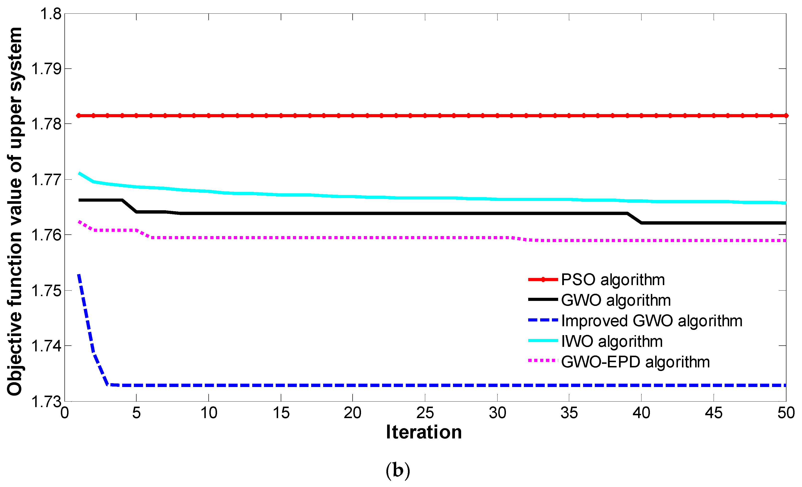
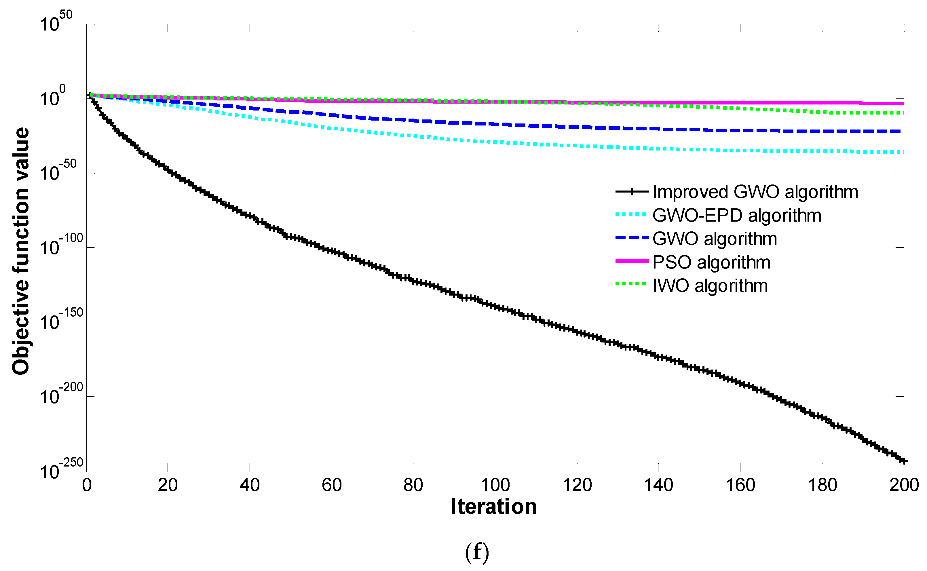
4.2. Verification of the Superiority of the Improved GWO Algorithm

An optimal simulation was performed to test the optimal ability of the improved GWO algorithm. A single-mode function and multi-mode function were selected for the test [35,36,37,38]. $f_1(x)$, $f_2(x)$, and are single-mode functions that represent the typical method of evaluating the global convergence of an algorithm. $f_4(x)$, $f_5(x)$, and $f_6(x)$ are multi-mode functions, which are typically used to evaluate the development performance, and searching ability of the algorithm. This function contains additional local minimums. The solution process easily reached a local optimal solution, and the optimal result was not easily obtained. The test function dimension was set to 10, and the corresponding expression is shown in

Table 2. Test functions.

Test Function	Search Scope
$f_1(x)={\displaystyle \sum _{i=1}^n\left|x_i\right|}+{\displaystyle \prod _{i=1}^n\left|x_i\right|}$	[−10, 10]
$f_2(x)={\displaystyle \sum _{i=1}^{n}i{x}_i^4+random[0,1]}$	[−1.28, 1.28]
$f_3(x)={\displaystyle \sum _{i=1}^n{x}_i^2}$	[−100, 100]
$f_4(x)={\displaystyle \sum _{i=1}^n[x_i^2-10\cos (2\pi x_i)+10]}$	[−5.12, 5.12]
$f_5(x)=-20\exp (-0.2\sqrt{\frac{1}{n}{\displaystyle \sum _{i=1}^n{x}_i^2}})-\exp (\frac{1}{n}{\displaystyle \sum _{i=1}^n\cos (2\pi x_i)})+20+e$	[−32, 32]
$f_6(x)=\frac{1}{4000}{\displaystyle \sum _{i=1}^n{x}_i^2-\prod \cos (x_i/\sqrt{i})+1}$	[−600, 600]

.

A comparison experiment featuring the particle swarm optimization (PSO) algorithm, the invasive weed optimization (IWO) algorithm [39], the grey wolf optimization (GWO) algorithm [31], the grey wolf optimization/evolutionary population dynamics (GWO-EPD) algorithm [40], and the improved GWO algorithm was performed. The parameters of the PSO algorithm were as follows: the proportional weight was $w=0.8$, the particle swarm size was $N=100$, the learning factor was $s_1=s_2=2$, and the maximum number of iterations was 200. The parameters of the IWO algorithm were as follows: the particle swarm size was $N=100$, the maximum number of iterations was 200, and the maximum and minimum number of seeds were five and two, respectively. The parameters of the GWO and GWO-EPD algorithms were as follows: the grey wolf swarm size was $N=100$, and the maximum number of iterations was 200. The parameters of the improved GWO algorithm were the same as those of the GWO algorithm, in addition to adopting the improved strategy in this study. Every test function was evaluated and solved using the above five types of algorithms. The simulation results are shown in Figure 5, where the ordinate is represented in logarithmic form.

According to Figure 5, in the process of optimizing the six test functions, the improved grey wolf optimization (GWO) algorithm, the grey wolf optimization/evolutionary population dynamics (GWO-EPD) algorithm, and the GWO algorithm exhibited better performance and a faster convergence rate than the basic particle swarm optimization (PSO) algorithm, and invasive weed (IWO) algorithm. Moreover, the improved GWO algorithm was more convergent than the GWO and GWO-EPD algorithms, and exhibited better optimization capabilities. The above conclusions verified the accuracy and superiority of the proposed algorithm.

5. Example Analysis

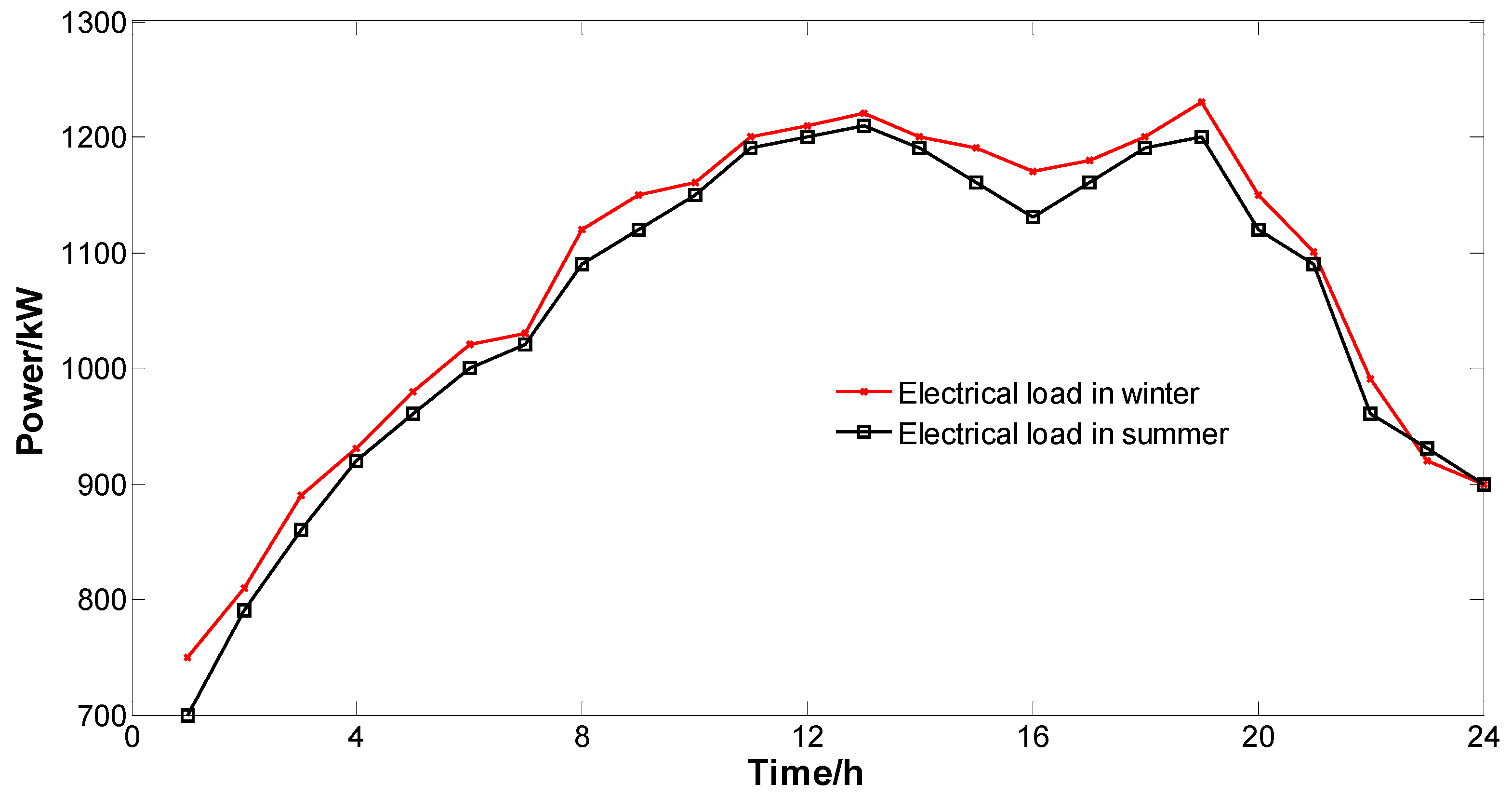
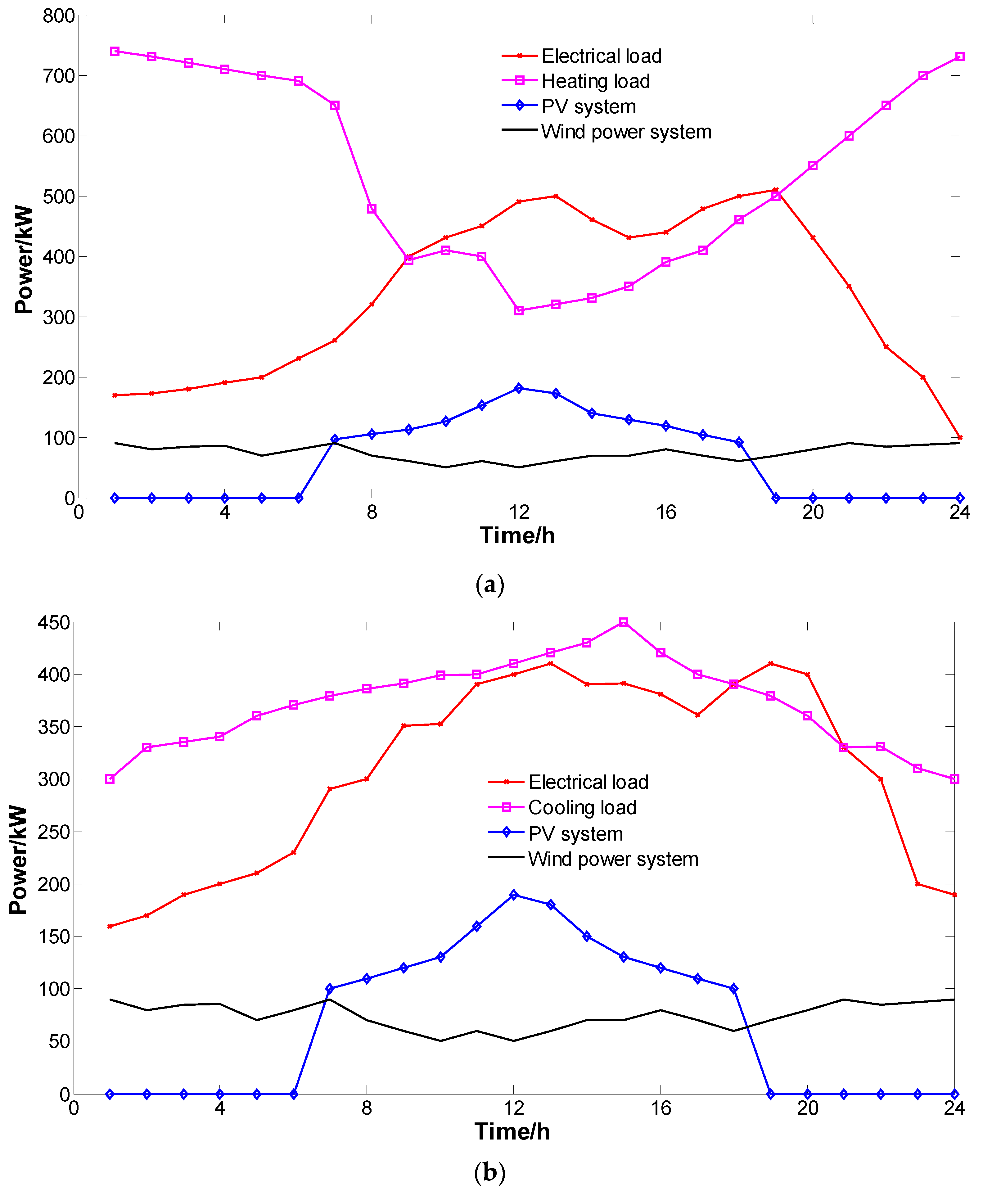
5.1. Overview of the Simulation System

An actual distribution network in a region of Gansu Province, China was used as an example to verify the model and algorithm proposed in this paper. The simulation system is shown in Figure 6. The waste-to-energy power stations were connected to nodes 19 and 23 in the system, and the maximum output power of the waste-to-energy power station was 600 kW. The micro energy grid of the agricultural park was connected to node 11, and the maximum exchanged power between the distribution network and the micro energy grid was 500 kW. The rated voltage of the lines was 10 kV, and the impedance of the lines is shown in

Table A1. Impedance of the lines.

Branch	Node		R (p.u.)	X (p.u.)
	From	To
1	0	1	0.491	0.295
2	1	2	0.104	0.137
3	2	3	0.104	0.135
4	3	4	0.126	0.167
5	4	5	0.033	0.042
6	5	6	0.223	0.294
7	6	7	0.198	0.261
8	7	8	0.124	0.163
9	8	9	0.229	0.221
10	9	10	0.231	0.226
11	10	11	0.307	0.215
12	11	12	0.195	0.059
13	1	13	0.491	0.295
14	2	14	0.135	0.058
15	3	15	0.271	0.116
16	4	16	0.272	0.113
17	5	17	0.269	0.223
18	6	18	0.198	0.085
19	18	19	0.198	0.085
20	18	20	0.792	0.341
21	7	21	0.099	0.043
22	21	22	0.098	0.042
23	22	23	0.096	0.049
24	23	24	0.961	0.391
25	8	25	0.333	0.152
26	25	26	0.267	0.125
27	25	27	0.083	0.037
28	10	28	0.352	0.217
29	28	29	0.301	0.152

. The simulation platform was MATLAB 2014a. The improved GWO algorithm was used to solve the model in this paper. The parameters of the algorithm were as follows: the grey wolf swarm size was $N=20$, and the maximum number of iterations was 50.

The power-supply equipment in the micro energy grid of the agricultural park included PV power, wind power, microturbines, gas-fired boilers, heat-recovery boilers, lithium-bromide absorption-type refrigerators, battery storage, heating and cooling storage tanks, and air-source heat pumps. The price of gas was 0.35 RMB/kW·h. The price of the power grid was determined using the peak and valley electricity prices issued by the Gansu Provincial Development and Reform Commission, as shown in

Table 3. Time-of-use electricity prices.

Period	Time	Buying Electricity Price/(RMB·kW·h−1)	Selling Electricity Price/(RMB·kW·h−1)
Peak period	08:00 a.m.–11:00 a.m., 06:00 p.m.–11:00 p.m.	0.7590	0.65
Flat period	07:00 a.m.–08:00 a.m., 11:00 a.m.–06:00 p.m.	0.5100
Valley period	11:00 p.m.–12:00 a.m., 12:00 a.m.–07:00 a.m.	0.2610

. The related environmental pollution parameters were provided in Reference [41]. The equipment parameters of the micro energy grid are provided in

Table 4. Storage equipment parameters of the micro energy grid.

Storage Equipment	Maximum Efficiency of Combined Electricity Heating and Cooling		Charged State of Combined Electricity Heating and Cooling		Lifespan/a	Capacity/(kW·h)	Initial Investment Cost/(RMB/kW)	Maintenance Cost/(RMB/kW·h)
	Charging	Discharging	Maximum	Minimum
Battery storage	0.2	0.2	0.9	0.2	5	1000	1100	0.03
heating and cooling storage tank	0.2	0.2	0.9	0.1	10	600	1200	0.02

and

Table 5. Supply equipment parameters of the micro energy grid.

Equipment	Parameter	Value	Equipment	Parameter	Value
Microturbine(four)	Maximum generated power/(kW·one−1)	100	Gas-fired boiler	Maximum input power/kW	200
	Rated efficiency	0.26		Rated efficiency	0.8
	Maintenance cost/(RMB/kW·h)	0.03		Maintenance cost/(RMB/kW·h)	0.02
	Initial investment cost/(RMB/kW)	5000		Initial investment cost/(RMB/kW)	2500
	Lifespan/a	10		Lifespan/a	10
	Ramp speed/(kW/min)	Upper 30 Lower 20		Ramp speed/(kW/min)	Upper 30 Lower 20
Heat-recovery boiler	Maximum input power/kW	480	Air-source heat pump	Maximum input power/kW	600
	Rated efficiency	0.9		Heating and cooling efficiency parameter	3.7
	Maintenance cost/(RMB/kW·h)	0.02		Maintenance cost/(RMB/kW·h)	0.02
	Initial investment cost/(RMB/kW)	3000		Initial investment cost/(RMB/kW)	3900
	Lifespan/a	10		Lifespan/a	10
Photovoltaic (PV) system	Maximum generated power/kW	300	Wind-power system	Maximum generated power/kW	100
	Maintenance cost/(RMB/kW·h)	0.03		Maintenance cost/(RMB/kW·h)	0.03
	Initial investment cost/(RMB/kW)	6500		Initial investment cost/(RMB/kW)	6300
	Lifespan/a	20		Lifespan/a	20
Exchanged power between the micro energy grid and the distribution network	Maximum exchanged power/kW	500	Lithium-bromide absorption-type refrigerator	Maximum input power/kW	576
				Rated efficiency	1.2
				Maintenance cost/(RMB/kW·h)	0.025
				Initial investment cost/(RMB/kW)	3000
				Lifespan/a	10

[7,41]. Load curves of the distribution network in the summer and in the winter are shown in Figure 7. The cooling, heating, and electrical load curves, and the wind power and PV prediction curves of the micro energy grid in the summer and in the winter are shown in Figure 8. The curves in Figure 7 and Figure 8 were simulated with Monte Carlo technology [42,43].

5.2. Analysis of the Simulation Results

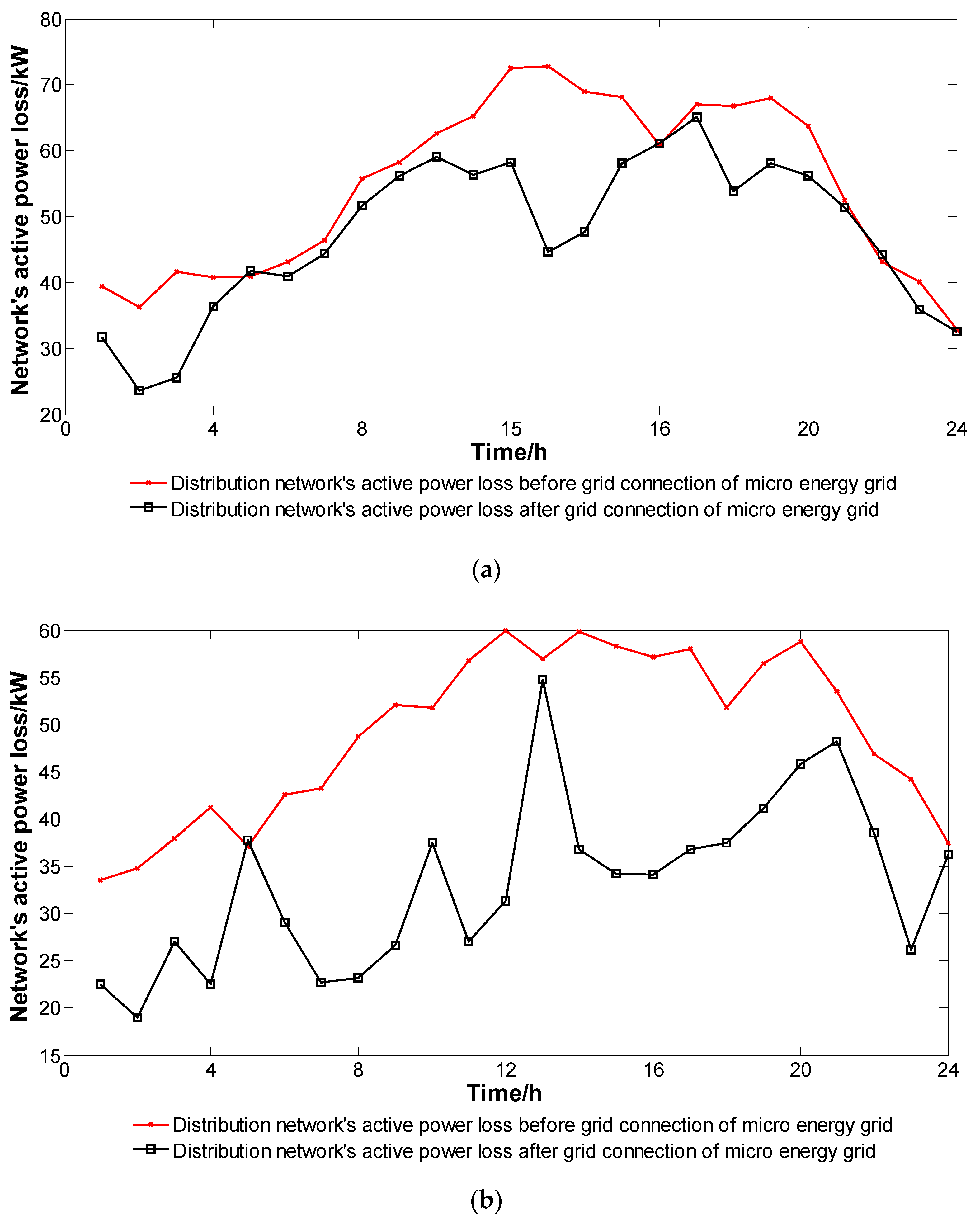
5.2.1. Active Power Loss Analysis of the Distribution Network Comprising the Micro Energy Grid

The network’s active power losses before and after the grid connection of the micro energy grid, on a typical day in the winter (a), and in the summer (b), are shown in Figure 9. The system network’s active power loss was larger when no micro energy grid was connected. However, when the micro energy grid was connected, and the proposed model was used, the average reduction in the network’s active power loss was 13.2% in the winter, and 32.4% in the summer. The network’s active power loss after the grid connection of the micro energy grid was significantly reduced when compared with that before the grid connection of the micro energy grid. The proposed model established the micro-energy-grid level needed to provide power support to the distribution-network level.

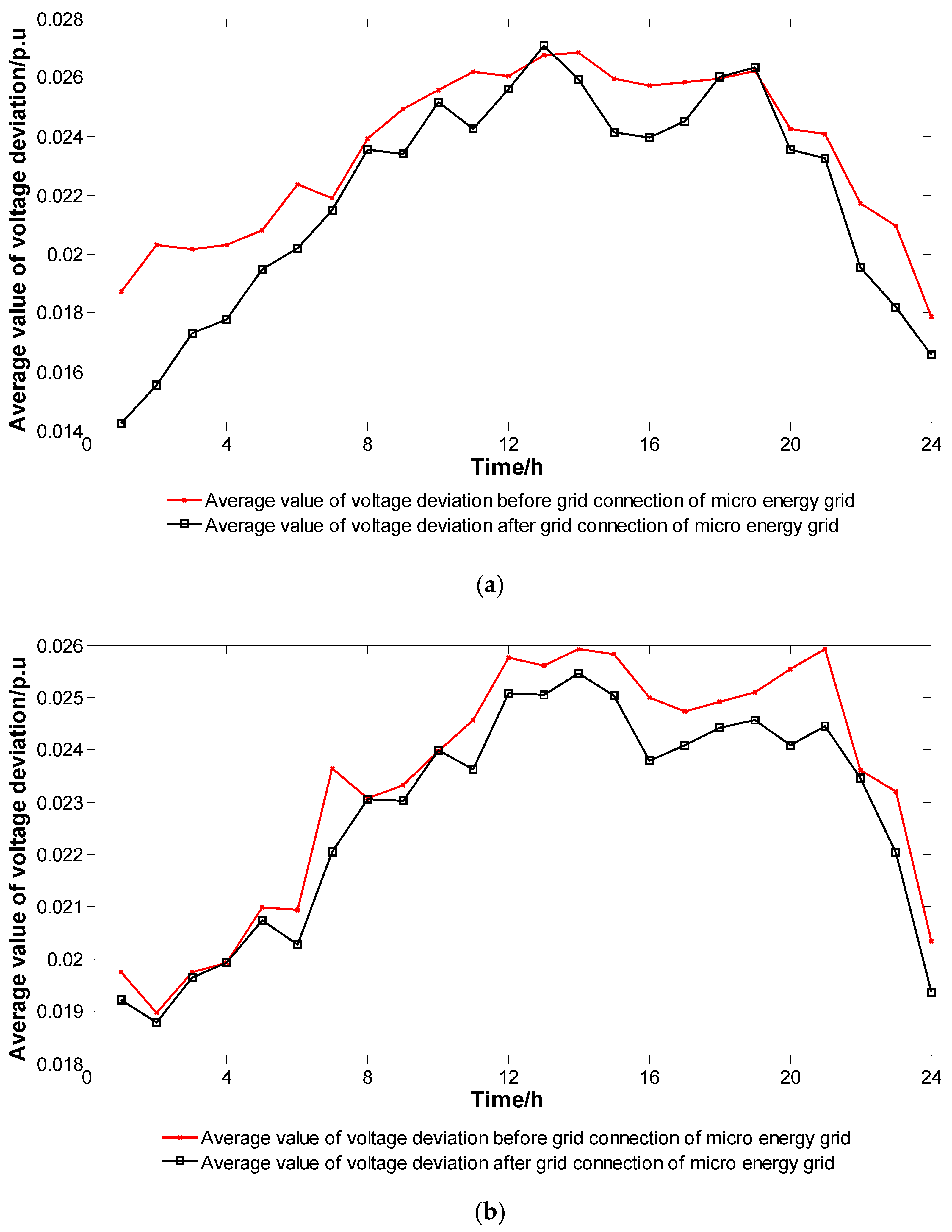
5.2.2. Voltage Deviation Analysis of the Distribution Network Comprising the Micro Energy Grid

The average voltage deviations before and after the grid connection of the micro energy grid, on a typical day in the winter (a), and in the summer (b), are shown in Figure 10. When the proposed model was used, the average reduction in the average voltage deviation was 6.4% in the winter, and 2.7% in the summer. The voltage fluctuation after the grid connection of the micro energy grid was significantly reduced when compared with that before the grid connection. The micro-energy-grid level supported the voltage of the distribution-network level, and improved the stability of the system voltage.

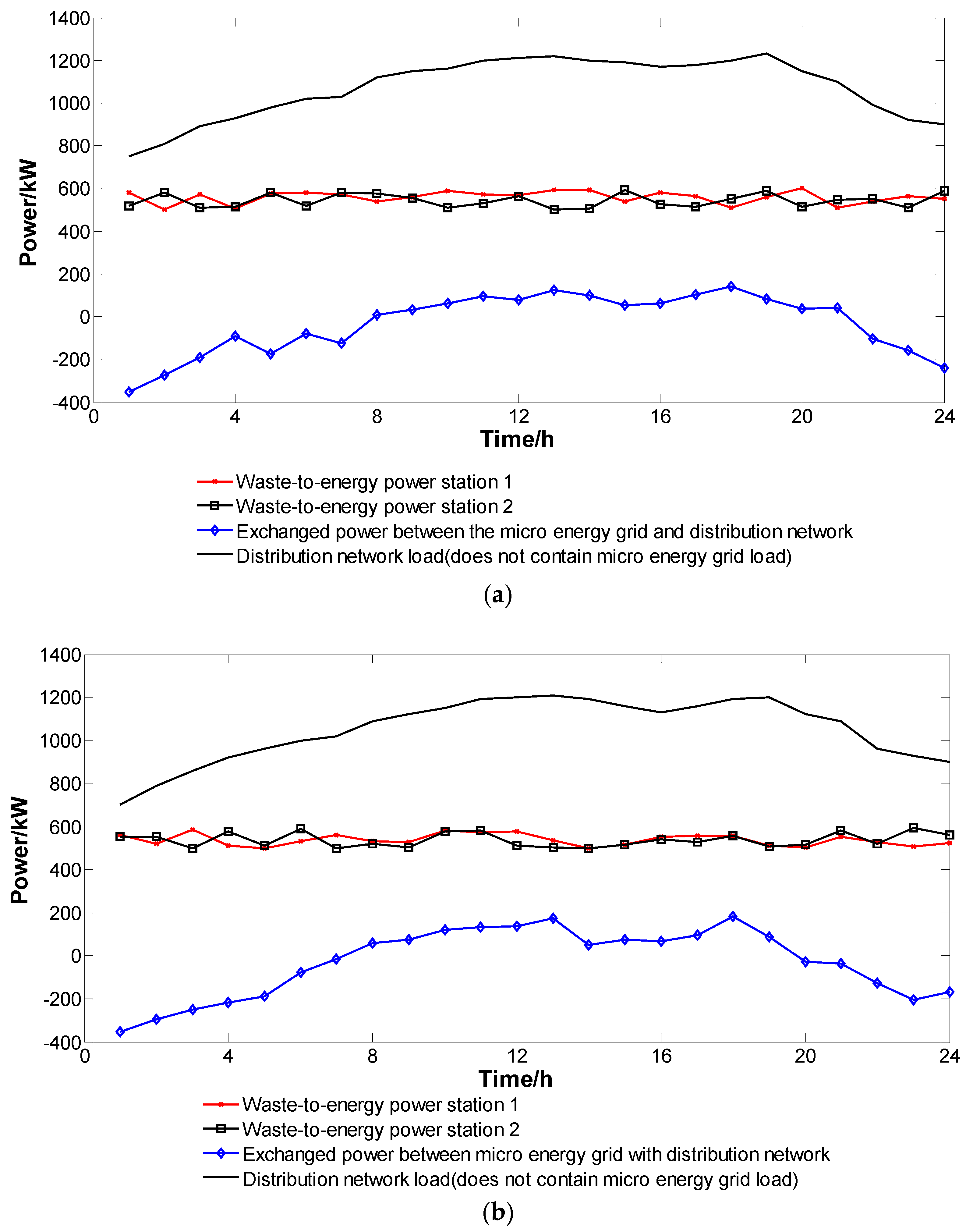
5.2.3. Optimal Dispatching Scheme of the Upper Distribution-Network Level

The optimal dispatching schemes of the distribution network comprising the micro energy grid, on a typical day in the winter (a), and in the summer (b), are shown in Figure 11. The micro energy grid bought electricity from the distribution network, which consumed the surplus power of the distribution network when the electricity price was in a valley period (11:00 p.m. to 07:00 a.m.). The micro energy grid sold its surplus electricity to the distribution network when the electricity price was in the flat or peak period (07:00 a.m. to 11:00 p.m.). The output power of the micro energy grid adapted to the load change in the distribution network, and played the role of peak load shifting in the distribution network. The micro energy grid effectively relieved the adjustment pressure of the unit in the distribution network, and allowed itself and the distribution network to gain the corresponding benefits.

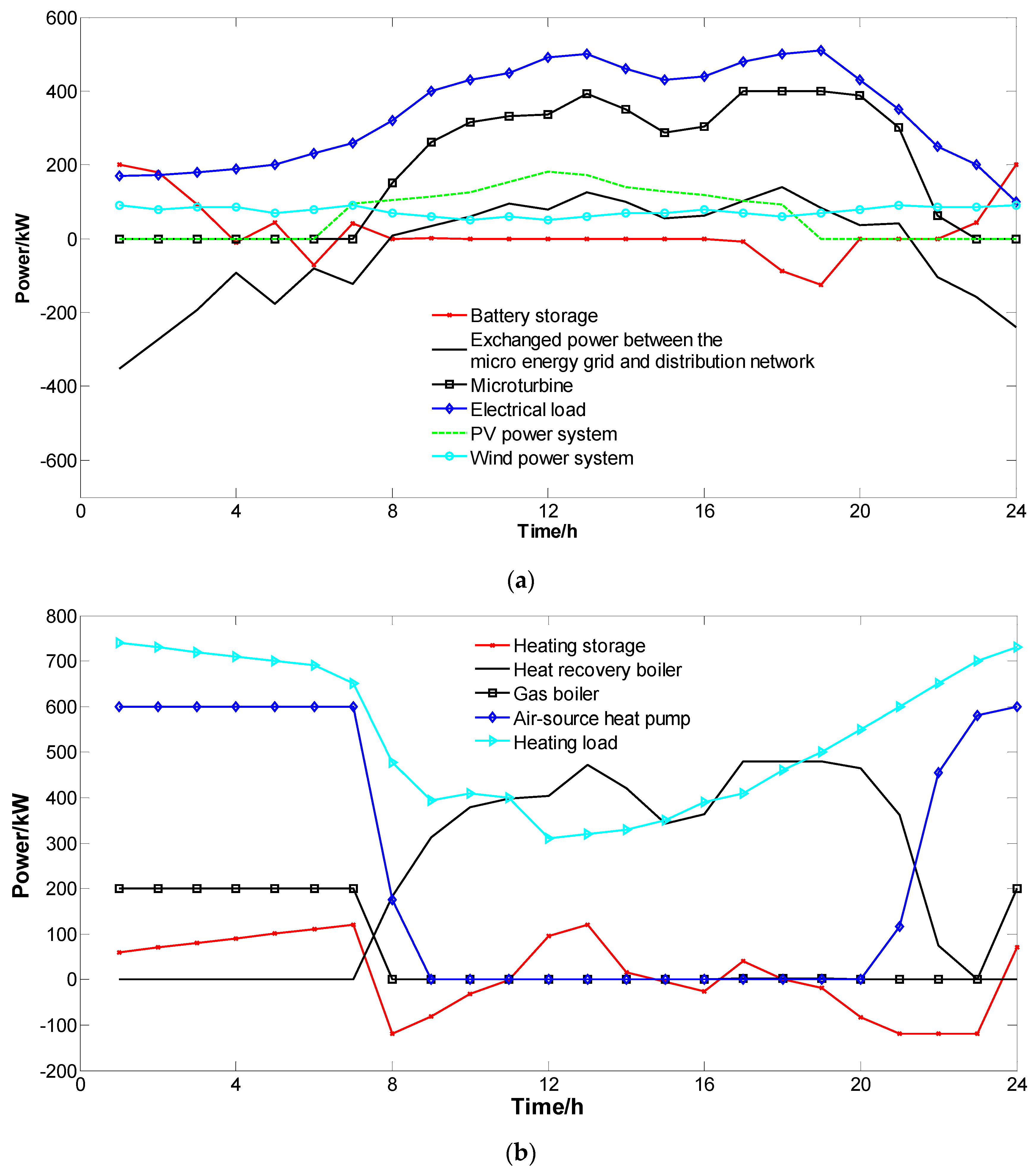
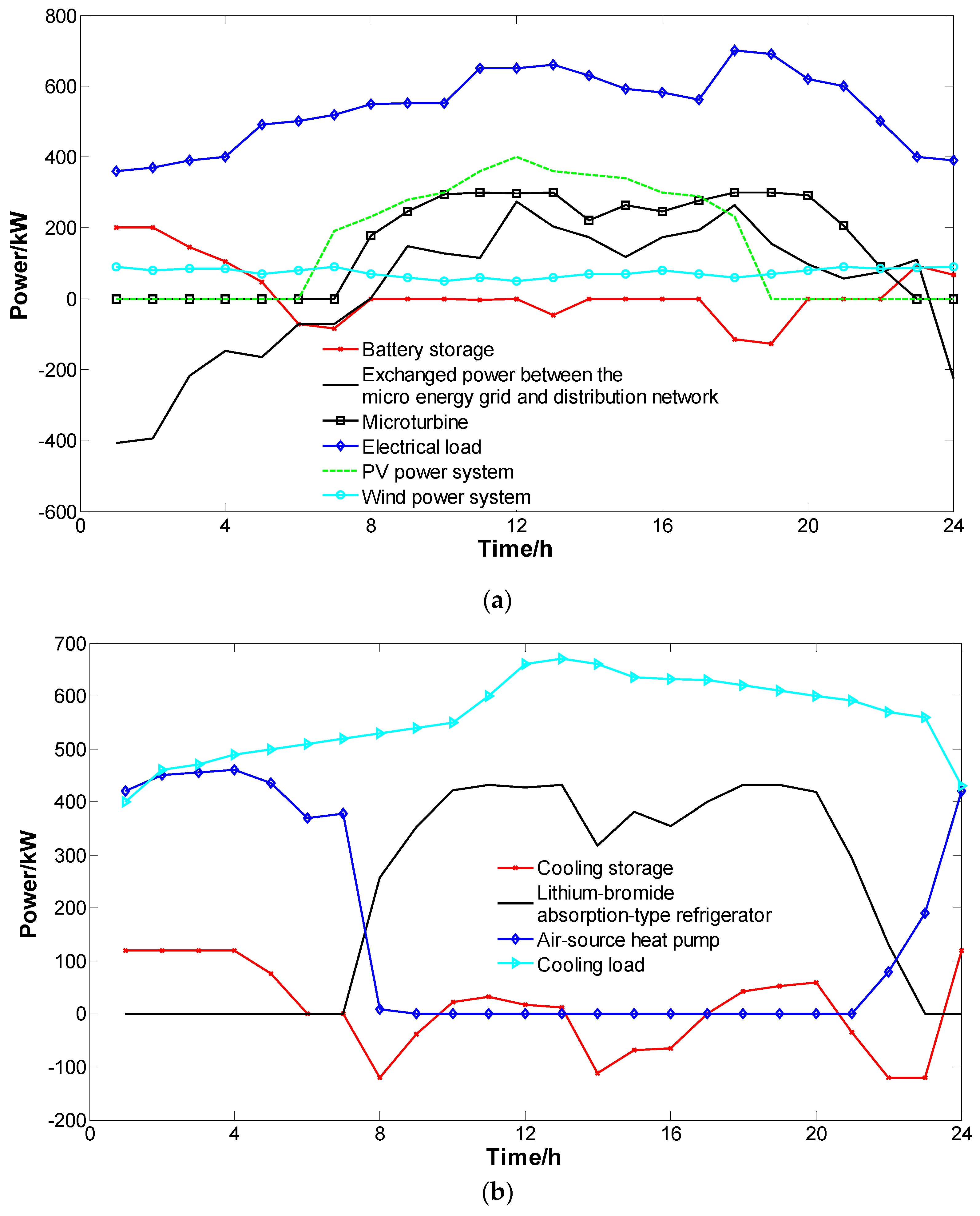
5.2.4. Optimal Dispatching Scheme of the Lower Micro-Energy-Grid Level

The electrical load (a) and heating load (b) dispatching schemes of the micro energy grid, for a typical day in the winter when the distribution network comprising the micro energy grid was in the optimal dispatching state, are shown in Figure 12. In Figure 12a, when PV and wind power could generate electricity, PV and wind power were at full power at the predicted output power, satisfying a portion of the energy needs of the micro energy grid. In the valley period of the electricity price, between 11:00 p.m. and 07:00 a.m., the microturbine did not work because the price of gas was higher than the electricity price of the power grid. Simultaneously, electricity was bought from the distribution network to satisfy the load demand, and to charge the battery. In the flat or peak period of the electricity price, between 07:00 a.m. and 11:00 p.m., the electricity load of the micro energy grid was satisfied by the microturbine, the discharge of the battery, and PV and wind power because the electricity price of the power grid was higher than the price of the gas. The surplus electricity was also sold to the distribution network to obtain income. During the entire running period, the battery was charged in the valley period, and discharged in the peak period, playing the role of peak load shifting in the micro energy grid, and reducing the operating cost of the micro energy grid.

In Figure 12b, the gas-fired boiler, heat-recovery boiler, battery storage, heating storage tank, and air-source heat pump jointly bore the supply of the heat load. In the valley period of the electricity price, between 11:00 p.m. and 07:00 a.m., the electricity price was low, and the air-source heat pump worked at full power. If the heat-recovery boiler and air-source heat pump could not satisfy the heat load, then the surplus heat-load demand was satisfied by the gas-fired boiler, and the heating storage tank was charged. In the flat or peak period of the electricity price, between 07:00 a.m. and 11:00 p.m., the electricity price was high, and the heating load was satisfied by the heat-recovery boiler, and the heat storage tank.

The electrical load (a) and cooling load (b) dispatching schemes of the micro energy grid, for a typical day in the summer when the distribution network comprising the micro energy grid was in the optimal dispatching state, are shown in Figure 13. In Figure 13a, because the load in the summer was less than the load in the winter, three microturbines were used in the summer, and the one remaining microturbine was overhauled. Similar to Figure 12a, when PV and wind power could generate electricity, PV and wind power were at full power at the predicted output power. In the valley period of the electricity price, between 11:00 p.m. and 07:00 a.m., the electricity was bought from the distribution network to satisfy the load demand, and to charge the battery. In the flat or peak period of the electricity price, between 07:00 a.m. and 11:00 p.m., the electricity load of the micro energy grid was satisfied by the microturbine, the discharge of the battery, and PV and wind power. Then, the surplus electricity was sold to the distribution network to obtain income. The battery storage played the role of peak load shifting in the micro energy grid.

In Figure 13b, the lithium-bromide absorption-type refrigerator, cooling storage tank, and air-source heat pump jointly bore the supply of the cooling load. In the valley period of the electricity price, between 11:00 p.m. and 07:00 a.m., the electricity price was low, and the air-source heat pump satisfied the cooling-load demand, and charged the cooling storage tank. In the flat or peak period of the electricity price, between 07:00 a.m. and 11:00 p.m., the electricity price was high, and the cooling load was mainly satisfied by the lithium-bromide absorption-type refrigerator and the cooling storage tank. If the lithium-bromide absorption-type refrigerator and the cooling storage tank could not satisfy the cooling load, then the surplus cooling-load demand was satisfied by the air-source heat pump.

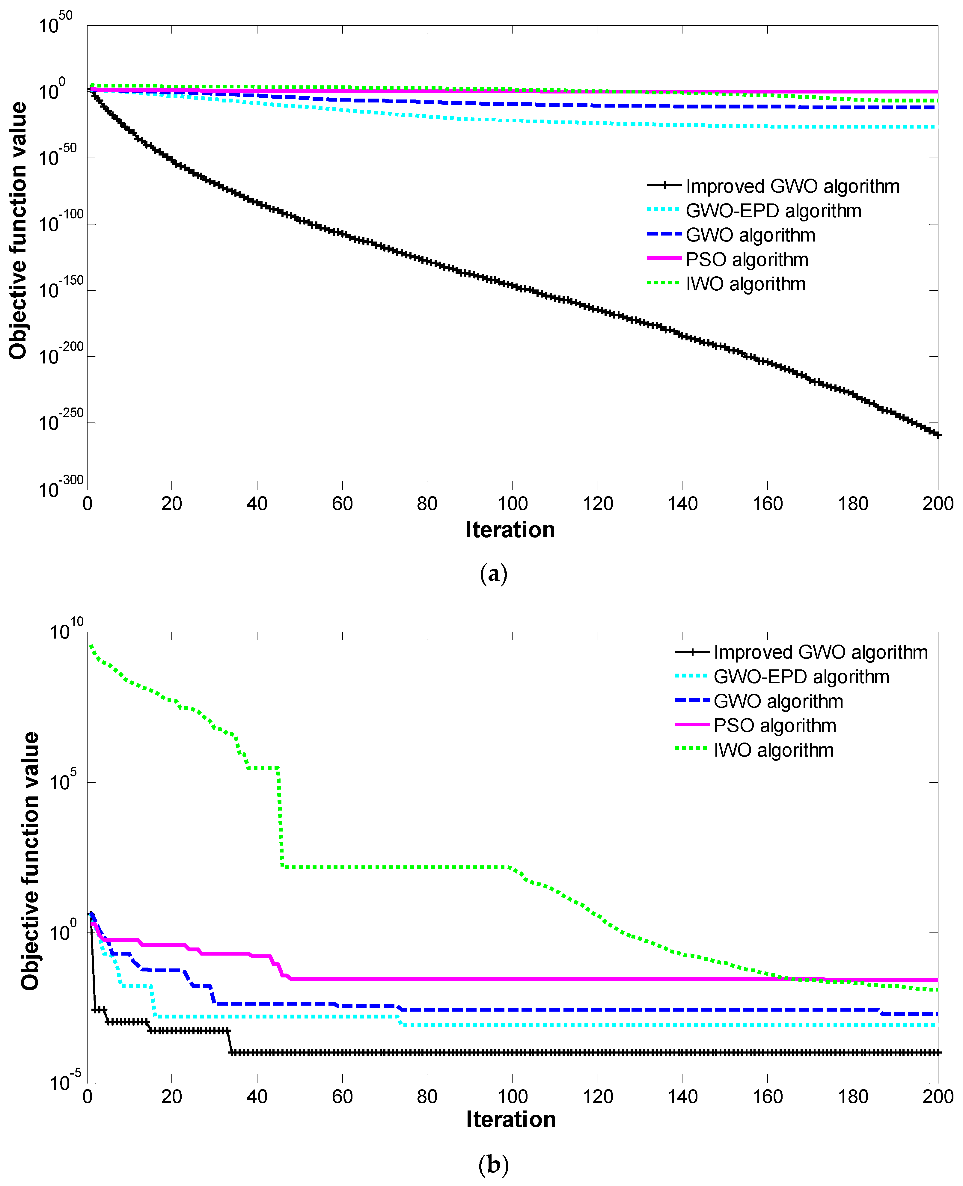
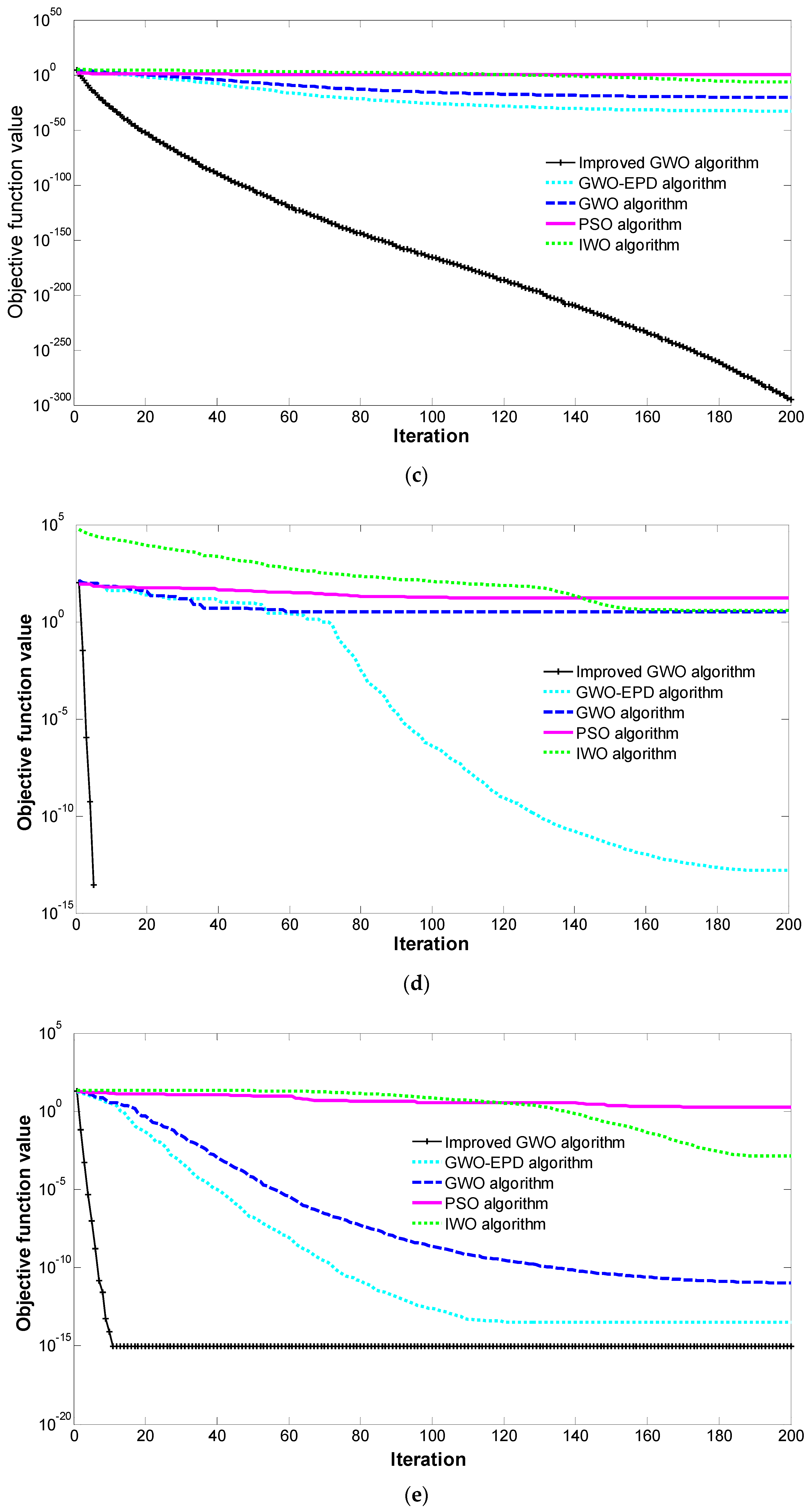
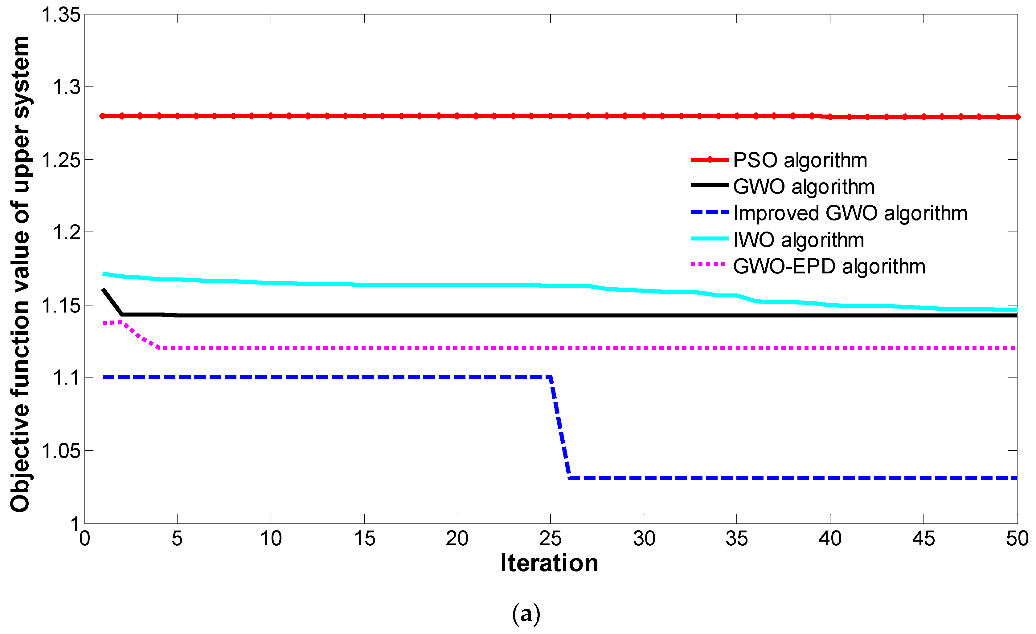
5.2.5. Performance Comparison of the Improved GWO Algorithm with the GWO, GWO-EPD, IWO, and PSO Algorithms

The optimal dispatching schemes of the distribution network comprising the micro energy grid, on a typical day in the winter (a), and in the summer (b), are shown in Figure 14. The objective function of the distribution-network level was normalized using the method presented in Section 3.1.3. In Figure 14, the particle swarm optimization (PSO) algorithm converged early, and often provided a local optimal solution. The optimal ability of the improved grey wolf optimization (GWO) algorithm was stronger than those of the PSO algorithm, invasive weed optimization (IWO) algorithm, grey wolf optimization/evolutionary population dynamics (GWO-EPD), and GWO algorithm. The fitness value of the objective function was significantly reduced by using the improved GWO algorithm. In the winter, the fitness value of the objective function with the improved GWO algorithm was reduced by 19.4% relative to that with the PSO algorithm, by 10.0% relative to that with the IWO algorithm, by 9.7% relative to that with the GWO algorithm, and by 7.9% relative to that with the GWO-EPD algorithm. In the summer, the fitness value of the objective function with the improved GWO algorithm was reduced by 2.7% relative to that with the PSO algorithm, by 1.8% relative to that with the IWO algorithm, by 1.6% relative to that with the GWO algorithm, and by 1.4% relative to that with the GWO-EPD algorithm.

5.2.6. Daily Cost Analysis of the Distribution Network Comprising the Micro Energy Grid Using the Improved GWO Algorithm, the GWO Algorithm, the GWO-EPD Algorithm, the IWO Algorithm, and the PSO Algorithm

According to

Table 6. Daily cost of the distribution network comprising the micro energy grid using five algorithms—the particle swarm optimization (PSO) algorithm, the invasive weed optimization (IWO) algorithm, the grey wolf optimization (GWO) algorithm, the improved GWO algorithm, and the GWO/evolutionary population dynamics (GWO-EPD) algorithm.

Algorithm	Cost of the Distribution Network (Does Not Contain Micro Energy Grid)/RMB		Cost of the Micro Energy Grid/RMB		Total System Cost/RMB
	Winter	Summer	Winter	Summer	Winter	Summer
PSO algorithm	1,126,004,317	39,809,957	94,318,029	3,292,247	1,220,322,346	43,102,204
IWO algorithm	750,401,055	39,040,023	71,295,926	3,273,691	821,696,981	42,313,714
GWO algorithm	741,777,648	38,852,914	68,603,822	3,266,733	810,381,470	42,134,740
GWO-EPD algorithm	740,359,725	38,717,692	65,104,632	3,253,778	805,464,357	41,971,470
Improved GWO algorithm	419,218,459	37,523,714	56,072,998	3,141,208	475,291,457	40,664,922

, when the improved grey wolf optimization (GWO) algorithm was adopted to optimize the operation of the distribution network comprising the micro energy grid, the cost of the distribution network, the cost of the micro energy grid, and the total cost of the system decreased considerably. In the winter, the cost of the distribution network, the cost of the micro energy grid, and the total cost of the system with the improved GWO algorithm were reduced by 62.7%, 44.1%, 43.4%, and 43.3%; 40.5%, 21.3%, 18.2%, and 13.8%; and 61.1%, 42.1%, 41.3%, and 40.9% relative to those with the particle swarm optimization (PSO) algorithm, the invasive weed optimization (IWO) algorithm, the GWO algorithm, and the grey wolf optimization/evolutionary population dynamics (GWO-EPD) algorithm, respectively. In the summer, the cost of the distribution network, the cost of the micro energy grid, and the total cost of the system with the improved GWO algorithm were reduced by 5.7%, 4.0%, 3.4%, and 3.0%; 4.6%, 4.0%, 3.8%, and 3.4%; and 5.6%, 3.8%, 3.4%, and 3.1% relative to those with the PSO algorithm, the IWO algorithm, the GWO algorithm, and the GWO-EPD algorithm, respectively.

5.2.7. Weight Sensitivity Analysis of the Objective Function of the Upper Distribution Network

In the upper distribution-network level, the weights $B=(0.5393,0.2974,0.1633)$ of multi-objective functions transformed into a single-objective function were obtained by expert experience in Section 3.1.3. To verify the influence on the operation state of the distribution network comprising the micro energy grid when the weight was changed, the sensitivity method was used to analyze the relevant problem. The relevant principle was shown in Reference [44]. The relationship equations between changes in weight, the weight sensitivity criteria, and the weight stable interval are shown in Formula (28). The conclusion is shown in

Table 7. Weight sensitivity analysis in the objective function of the upper distribution network.

Parameters	Weight of Total System Cost		Weight of Network‘s Active Power Loss		Standard Deviation of the Voltage Deviation
	Minimum	Maximum	Minimum	Maximum	Minimum	Maximum
Changes in weight	−0.1922	0.0463	−0.0928	0.3266	−0.0793	0.5894
Weight sensitivity criterion	0.3471	0.5856	0.2046	0.624	0.084	0.753
Weight stable interval	0.2385		0.4194		0.6687

.

$$\{\begin{array}{l}{G}_{\min }=B+\Delta M_{\min }\\ G_{\max }=B+\Delta M_{\max }\\ J=\Delta M_{\max }-\Delta M_{\min }\end{array},$$

(28)

where $B$ is the weight factor of the independent variable in the upper distribution-network level; $G_{\min }$ and $G_{\max }$ are the minimum and maximum weight sensitivity criteria; $\Delta M_{\min }$ and $\Delta M_{\max }$ are the minimum and maximum changes in weight; and $J$ is the weight stable interval.

According to the data of the weight stable interval in Table 7, the weight stable interval of total system cost was less than the weight stable interval of the network’s active power loss, which was less than the weight stable interval of the standard deviation of the voltage deviation. Relative to the system, the weight sensitivity of total system cost was greater than the weight sensitivity of network’s active power loss, which was greater than the weight sensitivity of the standard deviation of the voltage deviation. For the high-sensitivity weight, the objective function value was easily changed by a subtle change in the independent variable of the corresponding objective function. To keep the system running stably according to the current scheme, the weight selection range of total system cost was 0.3471–0.5856, the weight selection range of the network’s active power loss was 0.2046–0.624, and the weight selection range of the standard deviation of the voltage deviation was 0.084–0.753.

6. Conclusions

In this study, the operating structure of a distribution network comprising a micro energy grid was constructed. Based on the structure, a bi-level optimal dispatching model was established. The micro-energy-grid level used the minimum integrated operating cost of the micro energy grid as the objective function, while the distribution-network level used the minima of three objectives, including the integrated operating cost of the distribution network, the network’s active power loss, and the standard deviation of the voltage deviation in the distribution network. The judgment-matrix method was used to transform the multi-objective function of the distribution-network level into a single-objective function. A grey wolf optimization (GWO) algorithm, based on the dynamic adjustment of the proportional weight and convergence factor, was proposed to solve the economical operating model of the distribution network comprising the micro energy grid in this study. The superiority of the proposed algorithm was verified mathematically. The simulation results of the example were as follows:

(1) The improved grey wolf optimization (GWO) algorithm was used to identify a rational, global optimal solution of the objective function quickly and stably in the distribution network comprising the micro energy grid. In the winter, the fitness value of the objective function with the improved GWO algorithm was reduced by 19.4% relative to that with the particle swarm optimization (PSO) algorithm, by 10.0% relative to that with the invasive weed optimization (IWO) algorithm, by 9.7% relative to that with the GWO algorithm, and by 7.9% relative to that with the grey wolf optimization/evolutionary population dynamics (GWO-EPD) algorithm. In the summer, the fitness value of the objective function with the improved GWO algorithm was reduced by 2.7% relative to that with the PSO algorithm, by 1.8% relative to that with the IWO algorithm, by 1.6% relative to that with the GWO algorithm, and by 1.4% relative to that with the GWO-EPD algorithm.

(2) When the improved grey wolf optimization algorithm was adopted to optimize the operation of the distribution network comprising the micro energy grid, the cost of the distribution network, the cost of the micro energy grid, and the total cost of the system decreased considerably. In the winter, the cost of the distribution network, the cost of the micro energy grid, and the total cost of the system with the improved grey wolf optimization (GWO) algorithm were reduced by 62.7%, 40.5%, and 61.1%, respectively, relative to those with the particle swarm optimization (PSO) algorithm, by 44.1%, 21.3%, and 42.1%, respectively, relative to those with the invasive weed optimization (IWO) algorithm, by 43.4%, 18.2%, and 41.3%, respectively, relative to those with the GWO algorithm, and by 43.3%, 13.8%, and 40.9%, respectively, relative to those with the grey wolf optimization/evolutionary population dynamics (GWO-EPD) algorithm. In the summer, the cost of the distribution network, the cost of the micro energy grid, and the total cost of the system with the improved GWO algorithm were reduced by 5.7%, 4.6%, and 5.6%, respectively, relative to those with the PSO algorithm, by 4.0%, 4.0%, and 3.8%, respectively, relative to those with the IWO algorithm, by 3.4%, 3.8%, and 3.4%, respectively, relative to those with the GWO algorithm, and by 3.0%, 3.4%, and 3.1%, respectively, relative to those with the GWO-EPD algorithm.

(3) The adjustment pressure of the unit in the distribution network was effectively relieved after the micro energy grid was connected to the distribution network. The micro energy grid played the role of peak load shifting in the distribution network. The network’s active power loss was significantly reduced using the proposed method. The network’s active power loss decreased by an average of 13.22% in the winter, and 32.4% in the summer. The voltage fluctuations also decreased considerably, and the stability of the system voltage was improved. The average deviation decreased by 6.4% in the winter, and 2.7% in the summer.

Considering that the micro-energy-grid cluster, composed of several micro energy grids, is connected to the distribution network, the internal power coordination and optimal control of the micro-energy-grid cluster, the power coordination control between the micro-energy-grid cluster and the distribution network, and the economical operation mode of the distribution network comprising the micro-energy-grid cluster represent the future research directions.

References

1. Yun, H.B.; Zhang, C.; Deng, Z.Q.; Bian, H.F.; Sun, C.G.; Jia, C. Economic optimization for configuration and sizing of micro integrated energy systems. J. Mod. Power Syst. Clean Energy 2018, 6, 330–341. [Google Scholar]
2. Mohammadi, A.; Mehrtash, M.; Kargarian, A. Diagonal quadratic approximation for decentralized collaborative TSO+DSO optimal power flow. IEEE Trans. Smart Grid 2018, (in press). [Google Scholar] [CrossRef]
3. Bahrami, S.; Amini, M.H. A decentralized trading algorithm for an electricity market with generation uncertainty. Appl. Energy 2018, 218, 520–532. [Google Scholar] [CrossRef] [Green Version]
4. Stephen, C.; Pierluigi, M. Integrated electricity-heat-gas modeling and assessment, with applications to the Great Britain system. Part I: High-resolution spatial and Temporal heat demand modeling. Energy 2018, (in press). [Google Scholar] [CrossRef]
5. Solanki, B.V.; Raghurajan, A.; Bhattacharya, K.; Canizares, C.A. Including smart loads for optimal demand response in integrated energy management systems for isolated microgrids. IEEE Trans. Smart Grid 2017, 8, 1739–1748. [Google Scholar] [CrossRef]
6. Ojeda-esteybrd, M.; Rubio-barrosrg, R.; Vargasa, A. Integrated operation planning of hydrothermal power and natural gas systems with large scale storages. J. Mod. Power Syst. Clean Energy 2017, 5, 299–313. [Google Scholar] [CrossRef]
7. Xu, Q.S.; Zeng, A.I.; Wang, K. Day-ahead optimized economic dispatching for combined cooling, heating and power in micro energy-grid based on hessian interior point method. Power Syst. Technol. 2016, 40, 1657–1665. [Google Scholar]
8. Golden Concord Group Limited’s Multi-Complementary Project Is Selected as National Demonstration Project. Available online: http://paper.people.com.cn/zgnyb/html/2017-02/13/content_1750009.htm (accessed on 13 February 2017).
9. Determined to Forge Ahead, High-tech Blueprint. Available online: http://jsnews.jschina.com.cn/shms/201709/t20170907_1017177.shtml (accessed on 7 September 2017).
10. Napis, N.F.; Abd.kadir, A.F.; Khatib, T.; Hassan, E.E.; Sulaima, M.F. An improved method for reconfiguring and optimizing electrical active distribution network using evolutionary particle swarm optimization. Appl. Sci. 2018, 8, 804. [Google Scholar] [CrossRef]
11. Li, X.L.; Geng, G.F.; Ji, Y.Q.; Lu, L.Z. Operation strategy of battery energy storage system in distribution network with distributed generation. Power Autom. Equip. 2017, 37, 1–6. [Google Scholar]
12. Wang, Y.; Chen, M.; Zhang, M.; Ji, W.L.; Sun, X.J.; Luo, X.; Lan, L.; Gu, W. Distributed reactive power optimization for active distribution network based on equal incremental rate of network loss. Power Syst. Technol. 2017, 41, 1–9. [Google Scholar]
13. Fu, Y.; Liao, J.B.; Li, Z.K.; Qian, X.; Tang, X. Day-ahead optimal scheduling and operating of active distribution network considering violation risk. Proc. CSEE 2017, 37, 1–11. [Google Scholar]
14. Arshad, A.; Ekstrom, J.; Lehtonen, M. Multi-agent based distributed voltage regulation scheme with grid-tied inverters in active distribution networks. Electr. Power Syst. Res. 2018, 160, 180–190. [Google Scholar] [CrossRef]
15. Wang, W.; Huang, D.W. The coordination optimization of distribution networks with dispatched distributed generators. Trans. CES 2015, 30, 429–433. [Google Scholar]
16. Shukla, J.; Das, B.; Pant, V. Stability constrained optimal distribution system reconfiguration Uncertainties in correlated loads and distributed generations. Int. J. Electr. Power Energy Syst. 2018, 99, 121–133. [Google Scholar] [CrossRef]
17. Wang, L.; Sharkh, S.; Chipperfield, A. Optimal decentralized coordination of electric vehicles and renewable generators in a distribution network using A* search. Int. J. Electr. Power Energy Syst. 2018, 98, 474–487. [Google Scholar] [CrossRef]
18. Sheikhi, A.; Rayati, M.; Bahrami, S.; Ranjbar, A.M.; Sattari, S. A cloud computing framework on demand side management game in smart energy hubs. Int. J. Electr. Power Energy Syst. 2015, 64, 1007–1016. [Google Scholar] [CrossRef]
19. Amini, M.H.; Nabi, B.; Haghifam, M. Load management using multi-agent systems in smart distribution network. In Proceedings of the IEEE Power and Energy Society General Meeting, Vancouver, BC, Canada, 21–25 July 2013; pp. 1–5. [Google Scholar]
20. Li, C.B.; Zhang, J.Y.; Li, P. Multi-objective optimization model of micro-grid operation considering cost, pollution discharge and risk. Proc. CSEE 2015, 35, 1051–1058. [Google Scholar]
21. Huh, J.H.; Seo, K. Hybrid advanced metering infrastructure design for micro grid using the game theory model. Int. J. Softw. Eng. Appl. 2015, 9, 257–268. [Google Scholar] [CrossRef]
22. Yang, Y.; Lei, X.; Ye, T.; Li, T.; Xu, G.Y. Microgrid energy optimal dispatch considering the security and reliability. Proc. CSEE 2014, 34, 3080–3088. [Google Scholar]
23. Zhao, H.R.; Wu, Q.W.; Wang, C.S.; Cheng, L.; Rasmussen, C.N. Fuzzy logic based coordinated control of battery energy storage system and dispatchable distributed generation for microgrid. J. Mod. Power Syst. Clean Energy 2015, 3, 422–428. [Google Scholar] [CrossRef] [Green Version]
24. Armedariz, M.; Heleno, M.; Cardoso, G.; Mashayekh, S.; Stadler, M.; Nordstrom, L. Coordinated microgrid investment and planning process considering the system operator. Appl. Energy 2017, 200, 132–140. [Google Scholar] [CrossRef] [Green Version]
25. Xu, Y.T.; Ai, Q. Coordinated optimal dispatch of active distribution network with microgrids. Power Autom. Equip. 2013, 41, 143–149. [Google Scholar]
26. Fathi, M.; Bevrani, H. Statistical Cooperative Power Dispatching in Interconnected Microgrids. IEEE Trans. Sustain. Energy 2013, 4, 586–593. [Google Scholar] [CrossRef]
27. Wang, Z.Y.; Wang, J.H. Self-healing resilient distribution systems based on sectionalization into microgrids. IEEE Trans. Power Syst. 2015, 30, 3139–3149. [Google Scholar] [CrossRef]
28. Haddadian, H.; Noroozion, R. Optimal operation of active distribution systems based on microgrid structure. Renew. Energy 2017, 104, 197–210. [Google Scholar] [CrossRef]
29. Ameli, A.; Bahrami, S.; Khazaeli, F.; Haghifam, M. A multiobjective particle swarm optimization for sizing and placement of DGs from DG owner’s and distribution company’s viewpoints. IEEE Trans. Power Deliv. 2014, 29, 1831–1840. [Google Scholar] [CrossRef]
30. Mirjalili, S.; Mirjalili, S.M.; Lewis, A. Grey wolf optimizer. Adv. Eng. Softw. 2014, 69, 46–61. [Google Scholar] [CrossRef]
31. Jayakumar, N.; Subramanian, S.; Ganesan, S.; Elanchezhian, E.B. Grey wolf optimization for combined heat and power dispatch with cogeneration systems. Int. J. Electr. Power Energy Syst. 2016, 74, 252–264. [Google Scholar] [CrossRef]
32. Precup, R.E.; Davic, R.C.; Petriu, E.M. Grey wolf optimizer algorithm-based tuning of fuzzy control systems with reduced parametric sensitivity. IEEE Trans. Ind. Electron. 2017, 64, 527–534. [Google Scholar] [CrossRef]
33. Xiong, X.; Wang, J.B.; Jing, T.J.; Yang, R.G.; Ye, L. Power optimization control of microgrid cluster. Power Autom. Equip. 2017, 37, 10–17. [Google Scholar]
34. Zhao, X.; Zhao, C.Y.; Jia, X.F.; Li, G.Y. Fuzzy synthetic evaluation of power quality based on changeable weight. Power Syst. Technol. 2005, 29, 11–16. [Google Scholar]
35. Vascak, J. Adaptation of fuzzy cognitive maps by migration algorithms. Kybernetes 2012, 41, 429–443. [Google Scholar] [CrossRef]
36. Precup, R.E.; Sabau, M.C.; Petriu, E.M. Nature-inspired optimal tuning of input membership functions of takagi-sugeno-kang fuzzy models for anti-lock braking systems. Appl. Soft Comput. 2015, 27, 575–589. [Google Scholar] [CrossRef]
37. Ali, M.Z.; Awad, N.H.; Duwairi, R.M. Multi-objective differential evolution algorithm with a new improved mutation strategy. Int. J. Artif. Intell. 2016, 14, 23–41. [Google Scholar]
38. Chen, Z.M.; Zhou, S.R.; Luo, J.T. A robust ant colony optimization for continuous functions. Expert Syst. Appl. 2017, 81, 309–320. [Google Scholar] [CrossRef]
39. Castillo, C.A.; Conde, A.; Shih, M.Y. Improvement of non-standardized directional overcurrent relay coordination by invasive weed optimization. Electr. Power Syst. Res. 2018, 157, 48–58. [Google Scholar] [CrossRef]
40. Saremi, S.; Mirjalili, S.Z.; Mirjalili, S.M. Evolutionary population dynamics and grey wolf optimizer. Neural Comput. Appl. 2015, 26, 1257–1263. [Google Scholar] [CrossRef]
41. Ma, X.Y.; Wu, Y.W.; Fang, H.L.; Sun, Y.Z. Optimal sizing of hybrid solar-wind distributed generation in an islanded microgrid using improved bacterial foraging algorithm. Proc. CSEE 2011, 31, 17–25. [Google Scholar]
42. Xian, X.; Fan, C.G.; Wen, S.S.; Wang, Y.C.; Chen, C.; Liu, X. Optimal deployment for island microgrid considering probabilistic factors of renewable energy generations. Eng. J. Wuhan Univ. 2016, 49, 101–104. [Google Scholar]
43. Pazouki, S.; Haghifam, M.R.; Moser, A. Uncertainty modeling in optimal operation of energy hub in presence of wind, storage and demand response. Int. J. Electr. Power Energy Syst. 2014, 61, 335–345. [Google Scholar] [CrossRef]
44. Yang, L.; Sun, Z.L.; Yin, M.A.; Wang, Y.N. Optimization design of cartridge pressing structure for feed mechanism based on the sensitivity analysis of multi-attribute decision making. Acta Armamentarii 2014, 35, 241–247. [Google Scholar]
Figure 1. General workflow for the optimal operation of the distribution network comprising the micro energy grid, based on the improved grey wolf optimization (GWO) algorithm.
Applsci 08 00923 g001
Figure 2. Operating structure of a distribution network comprising a micro energy grid.
Applsci 08 00923 g002
Figure 3. Bi-level optimization model.
Applsci 08 00923 g003
Figure 4. Flow chart of the bi-level optimal model of the distribution network comprising the micro energy grid, based on the improved GWO algorithm.
Applsci 08 00923 g004
Figure 5. Result comparison of test function 1 (a); function 2 (b); function 3 (c); function 4 (d); function 5 (e); and function 6 (f) with five types of algorithms—the particle swarm optimization (PSO) algorithm, the invasive weed optimization (IWO) algorithm, the GWO algorithm, the improved GWO algorithm, and the GWO/evolutionary population dynamics (GWO-EPD) algorithm.
Applsci 08 00923 g005aApplsci 08 00923 g005bApplsci 08 00923 g005c
Figure 6. Simulation system.
Applsci 08 00923 g006
Figure 7. Electrical load curve of the distribution network on a typical day in the winter and in the summer.
Applsci 08 00923 g007
Figure 8. Cooling, heating, and electrical load curves, and wind power and photovoltaic (PV) prediction curves for the micro-energy grid on a typical day in the winter (a), and in the summer (b).
Applsci 08 00923 g008
Figure 9. Comparison of the network’s active power loss before and after the grid connection of the micro energy grid on a typical day in the winter (a), and in the summer (b).
Applsci 08 00923 g009
Figure 10. Comparison of the average voltage deviations before and after the grid connection of the micro energy grid on a typical day in the winter (a), and in the summer (b).
Applsci 08 00923 g010
Figure 11. Optimal dispatching schemes of the distribution network comprising the micro energy grid on a typical day in the winter (a), and in the summer (b).
Applsci 08 00923 g011
Figure 12. Electrical load (a) and heating load (b) dispatching schemes of the micro energy grid for a typical day in the winter when the distribution network comprising the micro energy grid was in the optimal dispatching state.
Applsci 08 00923 g012
Figure 13. Electrical load (a) and cooling load (b) dispatching schemes of the micro energy grid for a typical day in the summer when the distribution network comprising the micro energy grid was in the optimal dispatching state.
Applsci 08 00923 g013
Figure 14. Comparison of the optimal dispatching schemes of the distribution network comprising the micro energy grid on a typical day in the winter (a), and in the summer (b).
Applsci 08 00923 g014aApplsci 08 00923 g014b