A Modified Bayesian Network Model to Predict Reorder Level of Printed Circuit Board

Featured Application

The research was motivated by the requirement of a printed circuit board (PCB) manufacturer and the application of the work is to identify the repeated PCB orders for batch production according to the predicted reorder level.

Abstract

Identifying the printed circuit board (PCB) orders with high reorder frequency for batch production can facilitate production capacity balance and reduce cost. In this paper, the repeated orders identification problem is transformed to a reorder level prediction problem. A prediction model based on a modified Bayesian network (BN) with Monte Carlo simulations is presented to identify related variables and evaluate their effects on the reorder level. From the historically accumulated data, different characteristic variables are extracted and specified for the model. Normalization and principal component analysis (PCA) are employed to reduce differences and the redundancy of the datasets, respectively. Entropy minimization based binning is presented to discretize model variables and, therefore, reduce input type and capture better prediction performance. Subsequently, conditional mutual information and link strength percentage are combined for the establishment of BN structure to avoid the defect of tree augmented naïve BN that easily misses strong links between nodes and generates redundant weak links. Monte Carlo simulation is conducted to weaken the influence of uncertainty factors. The model’s performance is compared to three advanced approaches by using the data from a PCB manufacturer and results demonstrate that the proposed method has high prediction accuracy.

1. Introduction

A printed circuit board (PCB) is found in practically all electrical and electronic equipment. It is the base of the electronics industry [1]. Due to increased competition and market volatility, demand for highly individualized products promotes a rapid growth of orders with a small batch of purchase and production. Some orders even with the relatively large volume have been placed separately and repeatedly at different times by customers. Dynamic fluctuation of market demands for PCB can easily bring great production imbalance, which is a waste of production capacity during the idle period with fewer orders from customers. However, during the busy period, it results in tardiness among many orders. Multi-batches of the same PCB product produced separately always require higher preparation and production cost with a higher scrap rate. Identifying orders with high reorder frequency and combining different batches of these orders during a reasonable period (e.g., an idle period) as batch and inventory-oriented production can reduce production cost, benefit production capacity balance, and facilitate on time delivery.

Taking an example from a PCB manufacturer named Guangzhou FastPrint Technology Co., Ltd. (called FastPrint in this paper), few orders were manually selected each month for batch production during the idle period based on reorder frequency and cumulative delivery area in the past 30 months. The reorder frequency is the number of times a customer places the same type of orders to a manufacturer in a given period. The delivery area of each order corresponds to the amount (quantity) of PCB products the customer orders multiplied by the area of each piece of PCB. The cumulative delivery area is the accumulation of the delivery area of the same type of orders in a given period. If 80% of the manually selected orders for batch production can be purchased by customers within six months (i.e., the maximum storage period in the manufacturer’s inventory can be ordered by most of customers), then the manufacturer can profit from better utilization of idle resources and the reduction of repeated production preparation and cost. However, the manual selection process is experience-dependent and time-consuming. Meanwhile, the accuracy needs to be improved because only the reorder frequency and the cumulative delivery area are taken into consideration.

The selection of orders for batch production is not based on the accurate reorder frequency within a certain period but always according to the range of predicted reorder frequency (e.g., reorder frequency ≥ 3) in practice. Moreover, it is difficult to accurately determine the reorder frequency within a certain period for each PCB order in advance. Therefore, we transform the repeated orders identification problem into a reorder level prediction problem in which the reorder frequency within six months was divided into four reorder levels (i.e., 1, 2, 3, and 4) corresponding to the reorder frequency (0, 1–2, 3–5, and >5, respectively). On this basis, orders with a highly predicted reorder level corresponding to the range of high reorder frequency placed within six months are taken as candidates for batch production.

The reorder level prediction is similar to the data mining based customer identification (also referred to as customer acquisition) problem as an important task of customer relationship management (CRM) [2]. The former can be conducted by analyzing characteristics of the orders and subdividing them into different groups in which the order groups with higher reorder levels (e.g., 3 and 4) can be taken as candidates for batch production. The latter, on the other hand, is to seek the profitable customer segments by analyzing their underlying characteristics and subdividing an entire customer base into smaller customer segments, which are comprised of customers who are relatively similar within each specific segment [2,3]. Identification of the most profit-generating customers and segmentation of customers are quite vital [3]. Previous studies reveal that recency, frequency, and monetary (RFM) analysis and frequent pattern mining can be successfully used or integrated to discover valuable patterns of customer purchase behavior [3,4,5,6,7,8]. Dursun and Caber [3] took the RFM analysis for profiling profitable hotel customers and related customers were divided into eight groups. Chen et al. [4] incorporated the RFM concept to define the RFM sequential pattern and developed a modified Apriori for generating all RFM sequential patterns from customers’ purchasing data. Hu and Yeh [5] proposed RFM-pattern-tree to compress and store entire transactional database and developed a patterned growth-based algorithm to discover all the RFM-patterns in the RFM-pattern-tree. Coussement et al. [6] employed RFM analysis, logistic regression, and decision trees for the customers’ segmentation and identification. Mohammadzadeh et al. [7] employed k-means clustering for identifying target patient customers and then conducted the prediction of customers churn behavior via the RFM model based on the decision tree classifier. Song et al. [8] employed RFM considering parameters with time series to cluster customers and identify target customers.

Other data mining approaches have also been developed and many special factors were considered to excavate the customer pattern purchase behavior. Liu [9] developed a fuzzy text mining approach to categorize textual data to analyze consumer behaviors for the accurate classification of customers. Sarti et al. [10] presented a consumer segmentation method using clustering based on consumers’ purchase of sustainability and health-related products. Murray et al. [11] combined clustering with time series analysis to create customer segments and segment-level forecasts and then applied the forecasts to individual customers. Caigny et al. [12] proposed a logit leaf model for customer churn prediction in which customer segments are identified using decision rules and then a model is created for every segment using logistic regression. Ngai et al. [2] provided a comprehensive review of CRM from four dimensions such as customer identification, customer attraction, customer retention, and customer development. Zerbino et al. [13] presented a review of Big Data-enabled CRM including research on customer evaluation and acquisition. However, the topic discussed in this paper has seldom been studied to the best of our knowledge and it was not involved in the two previously mentioned reviews either.

Customer identification and a reorder level prediction are similar in that both of them aim to develop classified treatment strategy according to historical transactions. Nevertheless, there are differences from the following three aspects. First, the customer identification problem is to develop more accurate sales and advertising strategies based on customer transaction history and, therefore, better for retaining target customers [10] while the final purpose of the problem discussed in this paper is to select orders for batch production with different misclassification risks based on accumulated manufacturing orders. Second, RFM of different purchase products (orders) should be considered for the customer pattern mining while, in this research study, we only consider the parameters of the same product ordered at different times. Third, RFM are the main parameters considered in the customer identification problem while the production scale including quantity, area, and lifecycle of orders should also be considered in this paper. However, the previously mentioned approaches cannot be employed directly for reorder level prediction. Therefore, more influential variables and misclassification loss should be considered and related approaches should be developed.

In this paper, a prediction model based on modified Bayesian network (BN) with Monte Carlo simulations is presented to predict a reorder level of PCB orders. More precisely, we apply BN to excavate the relationship between influential variables (factors) and the reorder level. The main reason for choosing BN is that it has the clearest common sense interpretation and can be viewed as causal models of the underlying domains. It also owns the powerful capability of dealing with uncertainty and causality inference and has been widely used in predicting and classifying problems [14,15,16,17,18,19,20,21]. Figure 1 illustrates the framework of the proposed approach in which all procedures will be discussed in detail except for decision making marked with the dashed boxes.

The remainder of this paper is organized as follows. Relevant variables specification and data preprocessing including principal component analysis (PCA)-based factors extraction and entropy minimization-based data discretization are introduced in Section 2. The combination of conditional mutual information (CMI) and link strength percentage (LSP) to avoid the defect of tree augmented naïve (TAN) BN and conditional expected loss for final classification are described in Section 3. The model evaluation and comparison are given in Section 4 in which Monte Carlo simulation is conducted to determine the confidence upper limits of reorder frequency and weaken the influence of uncertainty factors. Additionally, performance of the proposed approach is compared to TAN, AdaBoost, and artificial neural networks (ANN). Conclusions are drawn in Section 5.

2. Variables Specification and Data Preprocessing

2.1. Variables Specification

Reorder level related variables were inherited and derived from fields in enterprise resource plan (ERP) system and order management system (OMS) in which the same type of repeated orders placed at different date are labeled with the same production number but different order numbers generated by the manufacturer’s coding rule. On this basis, statistics of delivery area, quantity, transaction money, and interval days of the past 30 months before a set date were derived and the related description is presented in

Table 1. Variable specification.

Variables	Symbols	Description
Layer number	Ln	PCB is made of resin, substrate, and copper foil and the Ln is the number of copper foil layers.
Continued days	Condays	Interval days between the first order date and a set date.
Recency	Rec	A period between the last order date and a set date.
Maximum/minimum/mean of delivery interval days	Delind_Max/Min/Mean	Days between order date and required delivery date in the past 30 months.
Maximum/minimum/mean of interval days	Interval_Max/Min/Mean	Days between two adjacent order dates in the past 30 months.
Frequency in 30 months	Fre3	Reorder frequency within 30 months before a set date.
Frequency	Fre	Reorder frequency before a set date.
Maximum/minimum/mean/sum of delivery area (m2)	Area_Max/Min/Mean/Sum	Delivery area of the past 30 months before a set date.
Maximum/minimum/mean/sum of money (CNY)	Mon_Max/Min/Mean/Sum	Transaction money of the past 30 months before a set date.
Maximum/minimum/mean/sum of delivery quantity	Qaun_Max/Min/Mean/Sum	Delivery quantity of the past 30 months before a set date.
Reorder level	Rel	1, 2, 3, and 4 levels corresponding to the reorder frequency 0, 1–2, 3–5, and >5 within six months, respectively.

Note: Statistic parameters of maximum/minimum/mean/sum were derived from the orders with the same production number accumulated in the past 30 months before a set date.

. The set date is prepared for orders selection and batch production. The statistic excludes the accumulation before 30 months under the consideration of order’s lifecycle based on expert experience. The reorder level is the classification objective and four levels are set based on the reorder frequency of a production number in the next six months after a set date.

Data from three factories accumulated in ERP and OMS of Fastprint were collected and integrated. Then 33,542 training samples were selected randomly with the set date 31 March 2016 based on the orders accumulated between 1 October 2013 and 31 March 2016. Meanwhile 14,484 test samples with another set date of 31 May 2016 were selected randomly based on the orders accumulated between 1 December 2013 and 31 May 2016 excluding the records with the same production number in training samples. The observed reorder levels for the records from training and test samples are transformed from the reorder frequency within six months after its set date (i.e., the frequency accumulated between 1 April 2016 and 30 September 2016 for training samples and between 1 June 2016 and 31 October 2016 for test samples). Each record was aggregated based on the orders placed during the past 30 months according to the production number. The records with reorder frequency 1 were not to be considered for batch production and have been deleted. Meanwhile few special orders with odd number layers and layer number greater than 20 have also been excluded because they are seldom taken for batch production in practice.

Sample size and the proportion of different reorder levels are presented in

Table 2. Samples and their proportion of different reorder levels.

Samples	Number (Proportion of Different Reorder Levels %)				Total Number
	1	2	3	4
All	38,678 (80.54)	6734 (14.02)	1777 (3.70)	837 (1.74)	48,026
Training	26,963 (80.39)	4735 (14.11)	1225 (3.65)	619 (1.85)	33,542
Test	11,715 (80.88)	1999 (13.80)	552 (3.80)	218 (1.52)	14,484

. It can be seen that sample proportions of different reorder levels are similar to those of the training and test samples, respectively. The statistic results show that only about 5.5% of the records with reorder level ≥ 3 in Table 2 in number were aggregated by a separately placed reorder. However, these small proportions of the records exerted significant influence on resource utilization and balance for the manufacturer in practice.

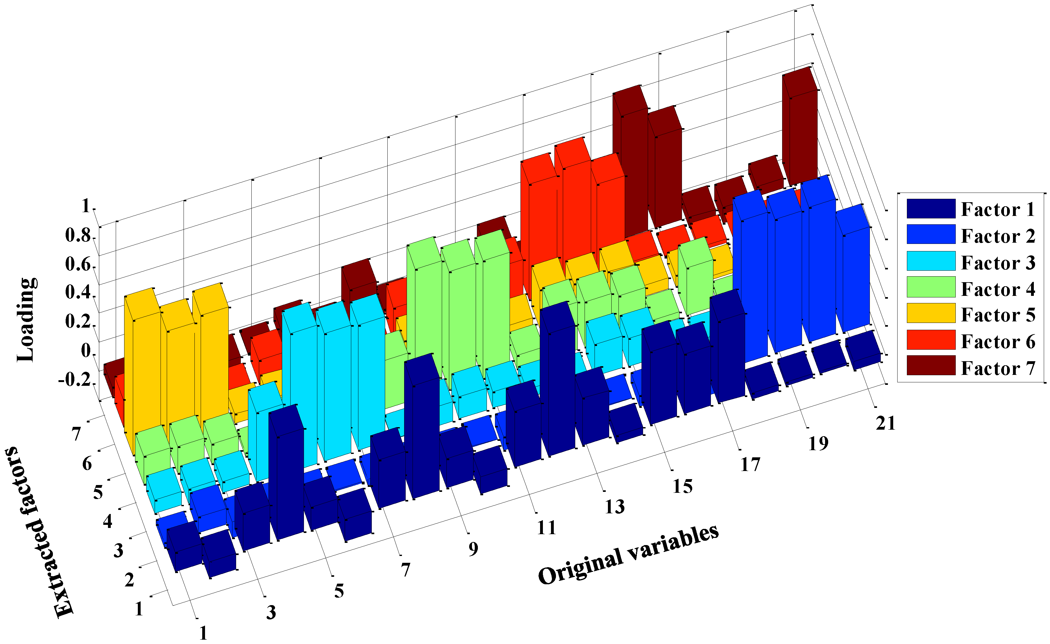
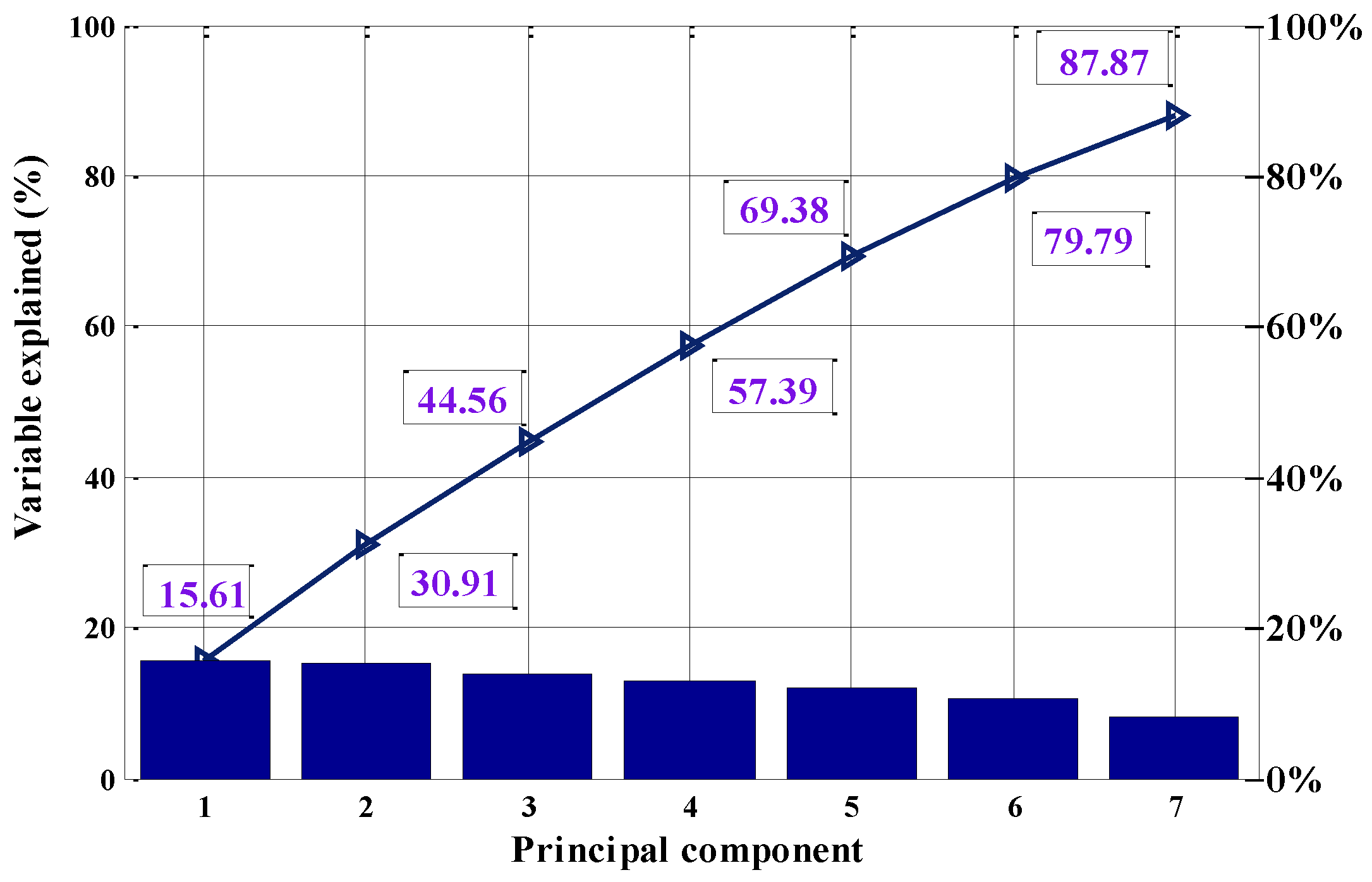
2.2. Principal Component Analysis

There are significant differences in values among variables given in Table 1. Some variables may be redundant or not have a significant influence on the reorder level prediction. Furthermore, continuous-valued variables with a large amount of input types easily generate too many conditional probability tables (CPTs) with sparse samples for each value, which negatively affects the establishment of a robust model. It is, therefore, necessary to perform preprocessing before building a model.

First, in order to eliminate the negative impact caused by the huge difference between each variable in terms of values, there is a need to normalize each variable ranging from 0 to 1. Second, the total data sample matrix 48,026 × 23 (i.e., the number of the samples multiplied by the number of the input variables for each records) would be considerably complicated and time consuming to model and test for such a high-dimension data samples [22]. It is, therefore, essential for reducing the dimension of the data samples and extracting the typical features from the original data samples. Third, in order to reduce input type and get better performance for variables, it is important to discretize variables for BN model development [14].

PCA is an effective statistical analysis method in multi-dimensional data compression and factors extraction. It can fuse relatively useful features and extract more sensitive factors through the evolution of the variance contribution rate and the cumulative variance contribution rate of each variable [22]. In this study, PCA was used for reducing variable redundancy for the proposed models. This could greatly reduce the modeling time and improve operational efficiency. The procedure of PCA is described below.

PCA was conducted by Algorithm 1 based on training samples according to the 21 input variables given in Table 1 except for the layer number and recency with some initial experiment. Seven factors were extracted with 87.87% of the cumulative variance contribution rate, which means the extracted factors can represent 87.87% of information of the original 21 input variables. The variance contribution rate and cumulative variance contribution rate are shown in Figure 2. The factor loading matrix with each loading $a_{ij}$ represents how many information factors $f_j$ can explain the variable $x_i$, which is illustrated in Figure 3. The numbers represent the original variables in Figure 3 and the main variables that each factor explained can be found in

Table 3. Number related variables and factor interpretation.

No.	Variables Name	Factors	Interpretation
1–3	Delind_Mean/Min/Max	1 (F1)	Qaun_Sum/Mon_Sum/Area_Sum
4–7	Qaun_Sum/Mean/Min/Max	2 (F2)	Interval_Mean/Min/Max, Condays
8–11	Mon_Sum/Mean/Min/Max	3 (F3)	Qaun_Mean/Min/Max
12–15	Area_Sum/Mean/Min/Max	4 (F4)	Mon_Mean/Min/Max
16–17	Fre/Fre3	5 (F5)	Delind_Mean/Min/Max
18–20	Interval_Mean/Min/Max	6 (F6)	Area_Mean/Min/Max
21	Condays	7 (F7)	Fre/Fre3/Condays

. On this basis, factor values of the test samples were computed based on the weighted sum of the original variables.

Algorithm 1. Factors extraction based on PCA.

(1) Normalization: For each column of the data sample $x_i$, min-max normalization was taken and $x_i^{\prime }=(x_i-x_{imim})/(x_{i\max }-x_{imim})$ was computed, where $x_i$ is the original data with $x_{imim}$ and $x_{i\max }$ representing the minimum and maximum values in $x_i$, respectively. (2) Principal component analysis: The calculation of the correlation coefficient matrix and its eigenvalues and eigenvectors was conducted. Subsequently, a variance explained matrix was constituted based on the eigenvectors. All the columns of this matrix were ranked according to the variance contribution rate in descending order. The cumulative variance contribution rate of principal components (factors) was calculated by ${\alpha }_m={\displaystyle \sum _{i=1}^m{\lambda }_i}/{\displaystyle \sum _{i=1}^n{\lambda }_i}$, where $\lambda$ is the eigenvalue of each dimension with $m$ representing the top $m$ principal components and ${\alpha }_m$ is the cumulative variance contribution. In this study, the top $m$ factors with a cumulative variance contribution rate of more than 85% were selected to replace the original $n$ variables. (3) Computing scores of factors. Scores of factors were computed according to the weight sum of original variables in which the weights were obtained based on least squares estimation.

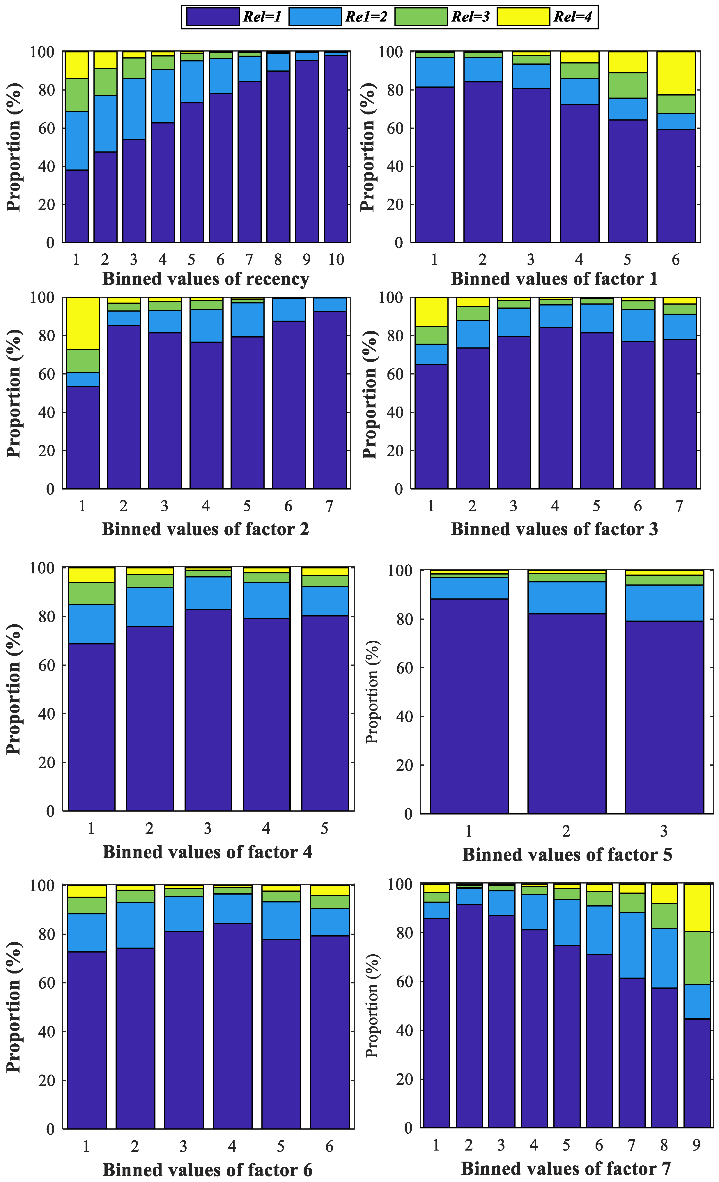
2.3. Data Discretization

The entropy minimization based binning method employed in this paper has been widely applied in discretizing variables [23]. The core measures of entropy minimization based discretization include information entropy and gain [24,25]. Let k classes be $C_1,C_2,\dots ,C_k$ in samples set S and let $P(C_i,S)$ be the proportion of samples in S that has class $C_i$. The entropy of $S$ is defined by the equation below.

$$Ent(S)=-{\displaystyle \sum _{i=1}^{k}P(C_i,S){\log }_{2}P(C_i,S)}$$

(1)

where Ent(S) measures the amount of information needed to specify the classes in S. The greater the Ent(S) value is, the more information it contains and the lesser purity it has. A binned interval with all values belonging to the same class has the highest purity [26,27].

Entropy of samples S partitioned by an arbitrary split point T of attribute $X$ into two disjoint intervals is defined by the equation below.

$$Ent(X,T;S)=={\displaystyle \sum _{j=1}^2\frac{|S_j|}{|S|}Ent(S_j)}$$

(2)

where $|S_j|$ and $|S|$ are the sample size of subset $S_j$ and $S$, respectively. The information gain for a variable $X$ based on a given split point $T$ can be defined by Equation (3).

$$Gains(X,T;S)=Ent(S)-Ent(X,T;S)$$

(3)

A partition induced by a split point T for a set S is accepted according to the minimum description length principle (MDLP) [24]. The binning algorithm for the discretization of each variable (i.e., F1–F7, layer number and recency) is described below.

The maximum number of the binned intervals was set to 10 and the discretization results of the variables obtained by Algorithm 2 are given in

Table 4. Discretized results of variables.

Variables (Factors)	Spilt Points
Ln	4, 10
Rec	11, 36, 67, 114, 172, 195, 325, 440, 714
F1	−0.09, 0.002, 0.211, 1.221, 2.436
F2	−0.767, −0.634, −0.496, 0.026, 0.787, 1718
F3	−0.532, −0.311, −0.251, −0.173, −0.024, 0.534
F4	−0.802, −0.481, −0.09, 0.872
F5	−0.1097, 0.443
F6	−0.879, −0.586, −0.329, 0.009, 1.432
F7	−1.009, 0.628, 0.386, 0.023, 0.401,1.335, 1.865, 3.501

. Split points were used directly for the discretization of the test samples. Proportions of the different reorder levels for the training samples in the different binned intervals of the variables are illustrated in Figure 4.

Algorithm 2. Entropy-based data discretization.

Input: Samples S, samples size N, variable $x$, classes of reorder level $\mathrm{Re}l=\{1,2,3,4\}$, and maximum number of binned interval MaxIntv. Output:   Split points for the variable $S{P}_x=\{s{p}_1,s{p}_2,\dots ,s{p}_{s-1}\}$, the number of final split point $s$, and binned values for variable $B_x=\{1,2,\dots ,s\}$ Iteration   Initialize empty set $S{P}_x$ and $B_x$;   Rank sample S according to $x$ in ascending order and the position $[1,\dots ,j,\dots ,N]$ are taken as its possible split points;   for k = 1 to MaxIntv;     Compute E(S) according to Equation (1); tempN = N; tempj = 0;     for j = 2 to $N$;      sp = 1; tempj = j   Get the value of $x$ at the position $j$ for (updated) sample S and suppose it is Tj;   $|S_j^1|$, $|S_j^2|$←the number of samples in the two intervals $S_j^1$ and $S_j^2$ separated by $T_j$; $|S_{j1}^l|$, $|S_{j2}^l|$, $|S_{j3}^l|$, $|S_{j4}^l|$←the number of samples with $\mathrm{Re}l=\{1,2,3,4\}$ in $S_j^l$, $l=1,2$, respectively;   $P(\mathrm{Re}{l}_k,S_j^l)=|S_{jk}^l|/|S_j^l|,1\le k\le 4$, $l=1,2$; Compute $E(S_j^l)$, $l=1,2$, $Ent(x,T_j;S)$, and $Gains(x,T_j;S)$ according to Equations (1)–(3) respectively;       if $Gains(x,T_j;S)$ satisfies MDLP;  Append $T_j$ to $S{P}_x$ and sp to $B_x$; sp ++; update $S\leftarrow S_j^2$, $N=|S_j^2|$; break;  end;  end;    if $tempj=tempN$; break; end;    end;   return $S{P}_x$ and $B_x$.

It can be seen that proportions of the different reorder levels in the different binned intervals vary significantly, which indicates that the cumulative delivery quantity/area (F1 and F3), delivery interval day (F5), and continued days (F2) are also important for classification of reorder level besides RFM (i.e. Rec, F7, and F4). Proportion of reorder level 2, 3, and 4 decreases with an increase in the value of discretized recency and the reorder level of the samples with the binned interval 10 for recency can almost directly be classified as 1. F7 performs the opposite tendency compared to recency in which the sample with the binned value 1 or 2 has high purity (probability) to be classified as 1. A sample with the binned recency as 1, F7 as 6, F2 or F3 as 1, or F7 as 9 has high probability to be classified as 4.

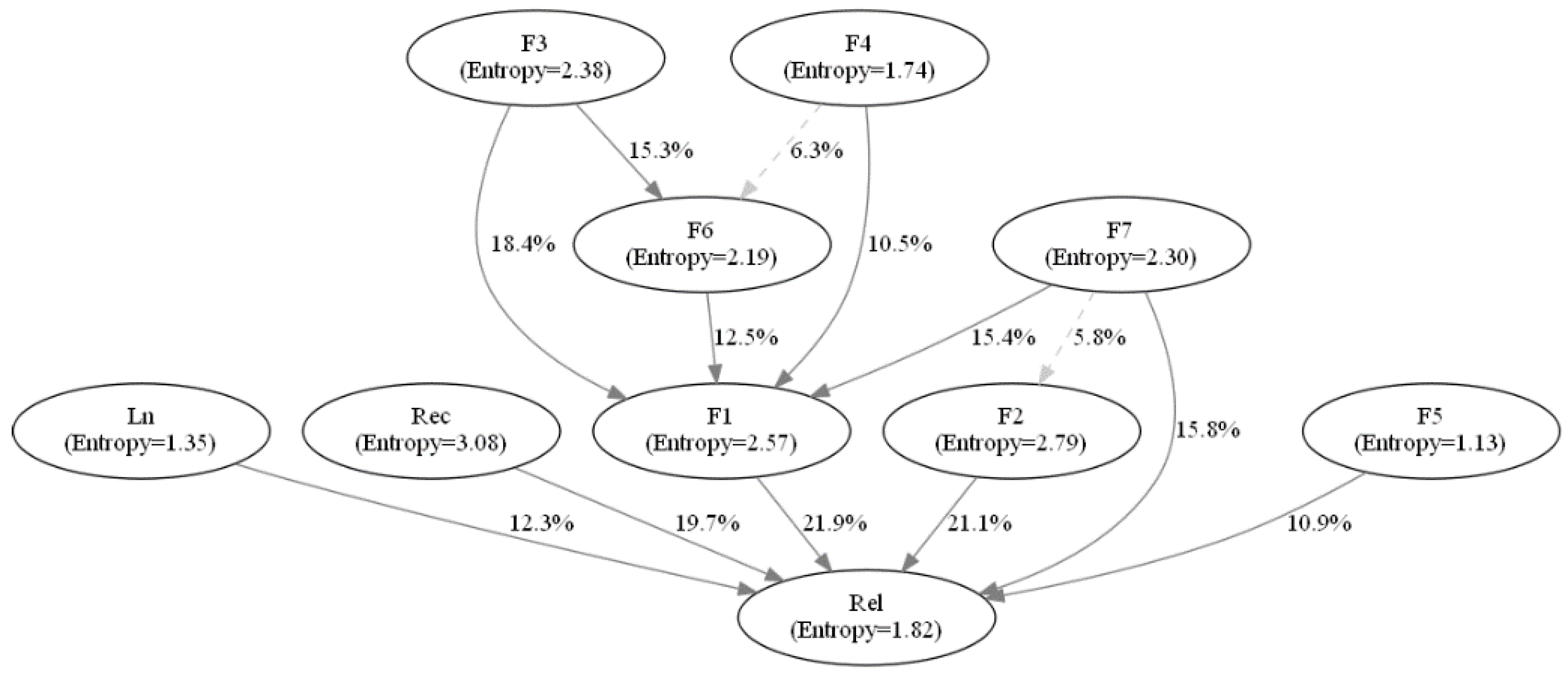
3. Modified Bayesian Network Model Development

3.1. Bayesian Network

Bayesian network (also known as belief network and causal network) is a probabilistic graphical model that represents a set of random variables and their conditional dependence by means of a directed acyclic graph (DAG) and CPTs [19,20]. Each node in DAG represents a variable of the ranges over a discrete set of domain and contacts with its parent’s nodes [14] and directed arcs represent the condition or probability dependency between random variables [14,28]. BN has become a popular knowledge-based representational scheme in data mining [27,28,29,30]. This graphical structure, which expresses causal interactions and direct/indirect relations as probabilistic networks, has secured BN’s popularity. Experts can easily understand such structures and (if necessary) modify them to improve the model [28].

The critical problem in establishing a BN is to determine the network structure S and corresponding set of parameters $\theta$ [28,29], which are always called structure learning and parameter learning, respectively. In order to reduce arcs between nodes (variables) with weak causal interactions and corresponding CPTs, CMI and LSP were combined with expert’s experience to establish BN structure and, therefore, avoid the defects of TAN. The CMI was first introduced in TAN [31] by relaxing the conditional independence assumption of naïve Bayesian for the purpose of selecting particular dependences [15]. However, TAN links all the input variables (evidence node) to output variables (class node) and allows at most two parents nodes with one connection to the class node and one causal connection to another evidence node, which easily misses some strong links and sometimes generates redundant weak strength links [28] that are negative for the robustness and generalization of the BN model.

Suppose a set of discretized random variables is $X=\{x_1,x_2,\dots ,x_9\}$ corresponding to the variables such as a layer number, recency, and F1–F7 and CMI between $x_i$ and $x_j$ can be computed below.

$$\mathrm{CMI}(x_i;x_j|\mathrm{Re}l)={\displaystyle \sum _{m,n,k}P(x_i^m,x_j^n,\mathrm{Re}{l}_k)}\ln \frac{P(x_i^m,x_j^n|\mathrm{Re}{l}_k)}{P(x_i^m|\mathrm{Re}{l}_k)P(x_j^n|\mathrm{Re}{l}_k)},i\ne j$$

(4)

where $x_i^m, x_j^n, \mathrm{and}\mathrm{Re}{l}_k$ represent the $m\mathrm{th}, n\mathrm{th},\mathrm{and}k\mathrm{th}$ values of $x_i^{}, x_j^{}, \mathrm{and}\mathrm{Re}l$, respectively. $\mathrm{CMI}(x_i; x_j|\mathrm{Re}l)$ measures the information $x_j$ provides on $x_i$ when the value of reorder level $\mathrm{Re}l$ is known. The smaller the $\mathrm{CMI}(x_i;x_j|\mathrm{Re}l)$ value is, the weaker the connection between $x_i$ and $x_j$ is.

The LSP from parent node $x$ to child node $y$ is defined by the equation below.

$$\mathrm{LSP}(x\to y)=100\times \frac{Ent(y|Z)-Ent(y|x,Z)}{Ent(y|Z)}$$

(5)

where $Z=P{a}_y/\left\{x\right\}$ denotes a set of all parents of $y$ other than $x$, $Ent(y|Z)={\displaystyle \sum _{z}P(z)}{\displaystyle \sum _{x_2}P(y|z)}{\log }_2(1/P(y|z))$, and $Ent(y|x,Z)={\displaystyle \sum _{x,z}P(x,z)}{\displaystyle \sum _{x_2}P(y|x,z)}{\log }_2(1/P(y|x,z))$. LSP can be interpreted by how much the uncertainty (in percentage) in class variable is reduced by knowing the state of an input variable if the states of all other parent variables are known. LSP plays an important role to evaluate the quality of the BN structure and can facilitate experts to modify arrows based on link strength values [32]. The structure learning algorithm is depicted below (Algorithm 3).

Algorithm 3. Modified BN structure establishment.

(1) Compute the $\mathrm{CMI}(x_i;x_j|\mathrm{Re}l)$ between $x_i$ and $x_j$ according to Equation (4); (2) Select input variables $x_{k1},\dots ,x_{kt}$ with $\mathrm{CMI}(x_i;x_j|\mathrm{Re}l)$ being greater than a threshold, and manually link $x_i$ to $x_{k1},\dots ,x_{kt}$ with directed arcs if there are no arcs between the two nodes; (3) Combining CMI by expert experience to determine the variables that links to Rel with directed arcs; (4) Compute LSP according to Equation (5) for each link to evaluate the quality of BN structure and modified (deleted) arrows with small LSP, e.g., 10%.

The Bayesian estimation method was employed for parameter learning in this paper to estimate $\theta =\max p(\theta |X)$ based on the training samples. Initially, $\theta$ was treated as a random variable and prior knowledge of $\theta$ is expressed as a prior probability distribution $p(\theta )$. Furthermore, there is a likelihood that the function was utilized based on samples. Subsequently, the Bayesian formula was taken to determine the posterior probability distribution of $\theta$. Dirichlet distribution was employed as the prior probability distribution of $p(\theta )$ [16].

CMI between $x_i$ and $x_j$ for the training samples based on Equation (4) is given in

Table 5. Conditional mutual information matrix.

Variables and Factors	Ln	Rec	F1	F2	F3	F4	F5	F6	F7
Ln	1	0.0018	0.002	0.0023	0.0703	0.0729	0.0307	0.0934	0.0023
Rec		1	0.01	0.019	0.005	0.041	0.0047	0.0108	0.0277
F1			1	0.0681	0.1004	0.141	0.0411	0.1098	0.1108
F2				1	0.0357	0.0125	0.0121	0.0226	0.1445
F3					1	0.099	0.041	0.2215	0.087
F4						1	0.0461	0.1121	0.0192
F5							1	0.0891	0.0144
F6								1	0.027
F7									1

. The threshold was set as 10% and CMI equal to or greater than 10% was reserved to construct the link. It can be seen that (1) CMI is small between layer number, recency, and F1–F7, which can be taken as independent variables while constructing BN structure. (2) CMI is large between F3, F4, F6, and F7, which means that the cumulative delivery scale (F1) of repeated orders is not independent of mean/min/max statistic results of delivery quantity, area, transaction money (F3, F6, and F4), and frequency (F7). (3) Similarly, F6 (mean/min/max delivery area) has great mutual information between F3 (mean/min/max delivery quantity) and F4 (mean/min/max transaction money).

On this basis, the structure of modified BN with entropy in each node and LSP for each link was constructed according to Algorithm 3, which was given in Figure 5. Entropy in each node reflects the purity of the node and they were computed based on $Ent(x)=-{\displaystyle \sum {}_{x_i}P(x_i){\log }_{2}P(x_i)}$ where $x_i$ is the discretized value set of node $x$, which indicates how much uncertainty is in $x$ if no evidence is given for any other nodes. LSP was computed based on Equation (5) and it can be seen that the LSP for links from Ln, Rec, F1, F2, F5, and F7 to Rel are large, which means that these variables can help reduce the high percentage of uncertainty for Rel when knowing the state of these nodes. Similarly, LSP of links from F2, F3, F6, and F7 to F1 are large, which indicates that F2, F3, F6, and F7 have a close causal relationship with F1. However, weak LSP of links from F7 to F2 and F4 to F6 marked with dotted lines are less than 10% and, therefore, the directed arcs from F7 to F2 and F4 to F6 were deleted accordingly. Then parameter learning was conducted based on the training samples and the structure to determine the CPTs for each node.

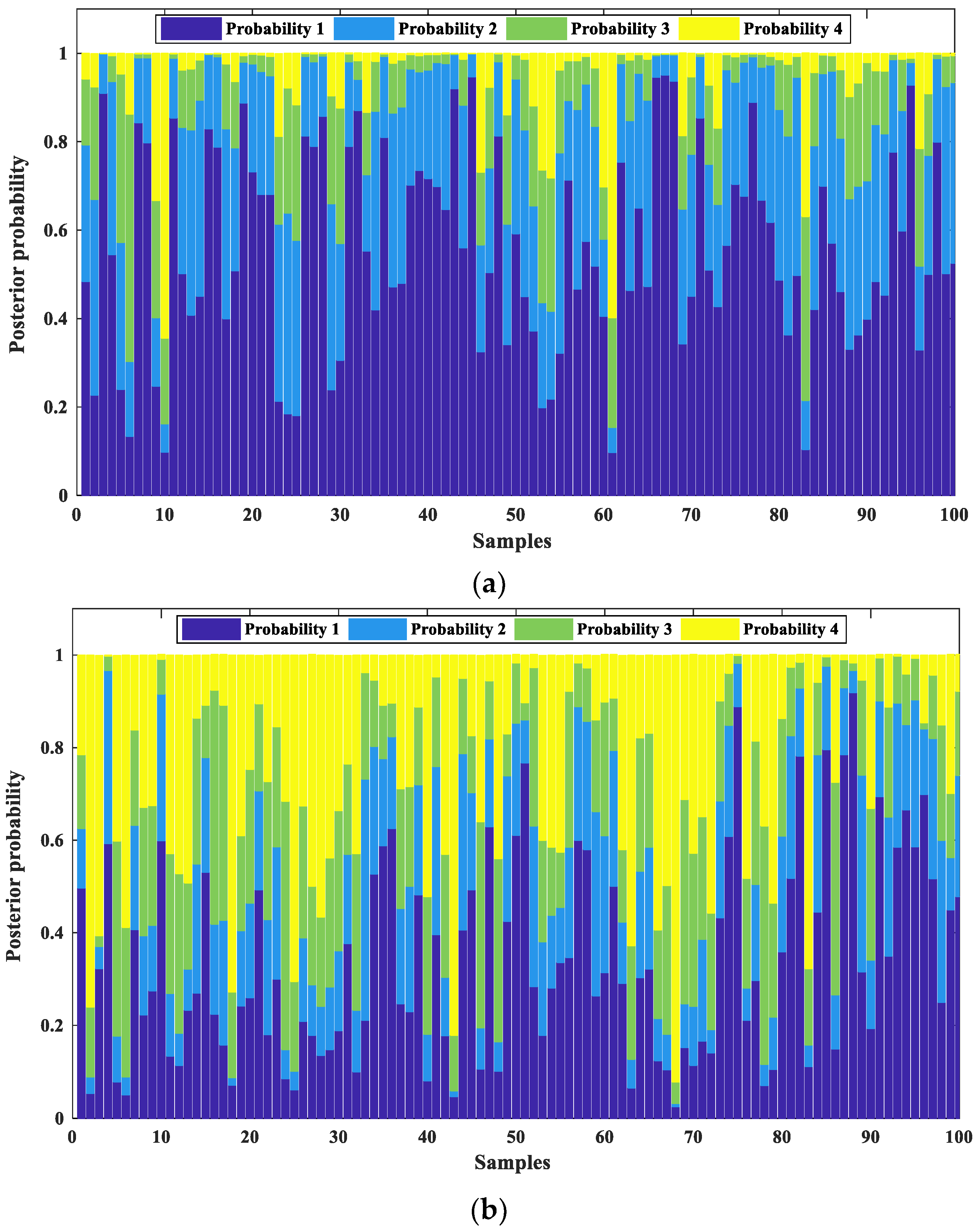
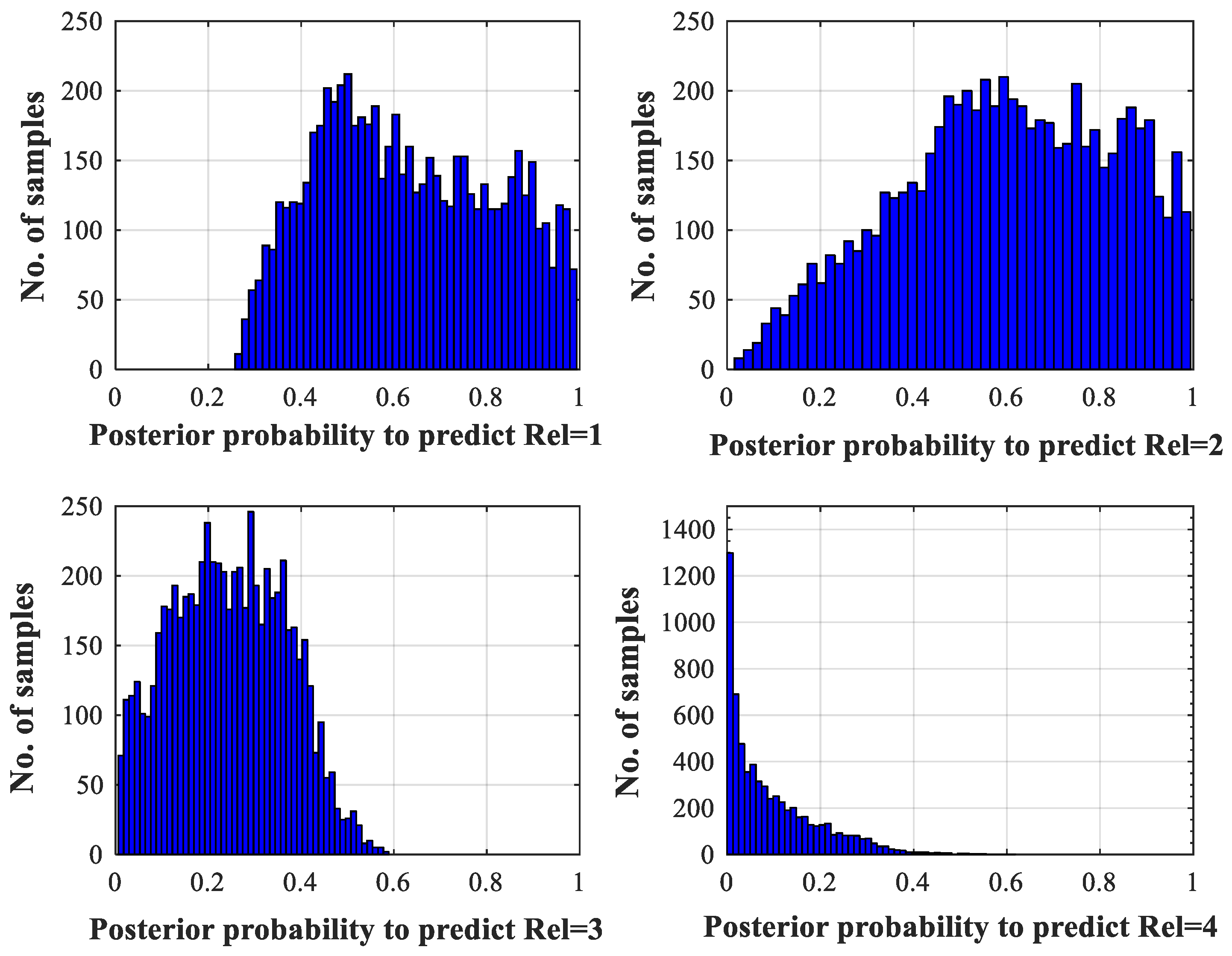
3.2. Conditional Expected Loss-Based Classification

Classification can be conducted based on learned BN structure and joint probability (the product of all the conditional probabilities of the network). Posterior probability of the reorder level can be calculated according to the Bayesian equation. Lastly, each sample can be predicted to the reorder level corresponding to the greatest posterior probability. However, a sample with a reorder level 1 misclassified as 2, 3, or 4 will bring economic risk if it is taken for batch production. At the same time, posterior probabilities of the biased reorder level may bring a different misclassification. Posterior probabilities of the training samples with observed reorder level 2, 3, or 4 based on the modified BN are given in Figure 6 according to initial experiments in which the posterior probabilities is generated by the formula below.

$$P(Pr\_\mathrm{Re}{l}_i|Ob\_\mathrm{Re}l=2,3,4)=\frac{P(Pr\_\mathrm{Re}{l}_i)P(Ob\_\mathrm{Re}l=2,3,4|Pr\_\mathrm{Re}{l}_i)}{{\displaystyle {\sum }_{j=1}^{4}P(Pr\_\mathrm{Re}{l}_j)P(Ob\_\mathrm{Re}l=2,3,4|Pr\_\mathrm{Re}{l}_j)}}$$

(6)

where $P(Pr\_\mathrm{Re}{l}_i)$ is the probability of predicted reorder level $i$ ($i=1,2,3,4$), $P(Ob\_\mathrm{Re}l=2,3,4)$ is the probability of observed reorder level with the value of 2, 3, or 4, $P(Ob\_\mathrm{Re}l=2,3,4|Pr\_\mathrm{Re}{l}_i)$ is the posterior probabilities of observed reorder level with the value of 2, 3, or 4 on the condition of the predicted reorder level $i$ and $P(Pr\_\mathrm{Re}{l}_i|Ob\_\mathrm{Re}l=2,3,4)$ is the posterior probabilities of predicted reorder level on the condition of observed reorder level as 2, 3, or 4. It can be seen that samples to be predicted as 3 and 4 are small and the corresponding posterior probabilities subjects to serious left skewed distribution with a mean value less than 0.25. In contrast, samples to be predicted as 1 or 2 are subject to right skewed distribution with a mean value greater than 0.5. This indicates that the posterior probability-based classification has high posterior probability to predict the reorder level of 1 with an observed value equal to or greater than 2 in many cases. Only a few instances with observed Rel = 3 or 4 have been predicted as 3 or 4.

Figure 7 illustrates the posterior probabilities of 100 randomly selected samples obtained by Equation (6) with observed Rel = 2 and Rel = 4 in which the probability of 1, 2, 3, and 4 corresponds to a predicted reorder level 1, 2, 3, and 4, respectively. Posterior probability in Figure 7a illustrates that it is easy to predict the reorder level of 2 to 1. Figure 7b illustrates that many posterior probabilities corresponding to the predicted reorder level 4 have no significant possibility for classifying it as 4. Therefore, the conditional expected loss was introduced instead of a posterior probability for the final classification decision. Let ${\alpha }_i$ be the decision to classify sample $X$ as ${\alpha }_i$, ${\lambda }_{ij}=\lambda ({\alpha }_i,{\omega }_j)$represents the loss (risk) to classify $X$ with observed value ${\omega }_j$ to ${\alpha }_i$, and all the ${\lambda }_{ij}=\lambda ({\alpha }_i,{\omega }_j)$ $i,j=1,2,3,4$, consist of classification loss matrix. Conditional expected loss is defined to illustrate the expected risk for a decision to predict $X$ as ${\alpha }_i$.

$$R\left({\alpha }_i|X\right)=E\left[\lambda \left({\alpha }_i,{\omega }_j\right)\right]={\displaystyle \sum _{j=1}^4\lambda \left({\alpha }_i,{\omega }_j\right)}P\left({\omega }_j|X\right),i=1,2,3,4.$$

(7)

The final decision can be conducted based on the minimization of the conditional expected loss.

$$R\left({\alpha }_k|X\right)=\underset{i=1,2,3,4}{\min }R\left({\alpha }_i|X\right)$$

(8)

The conditional expected loss-based classification can be described below (Algorithm 4).

Algorithm 4. Conditional expected loss-based classification.

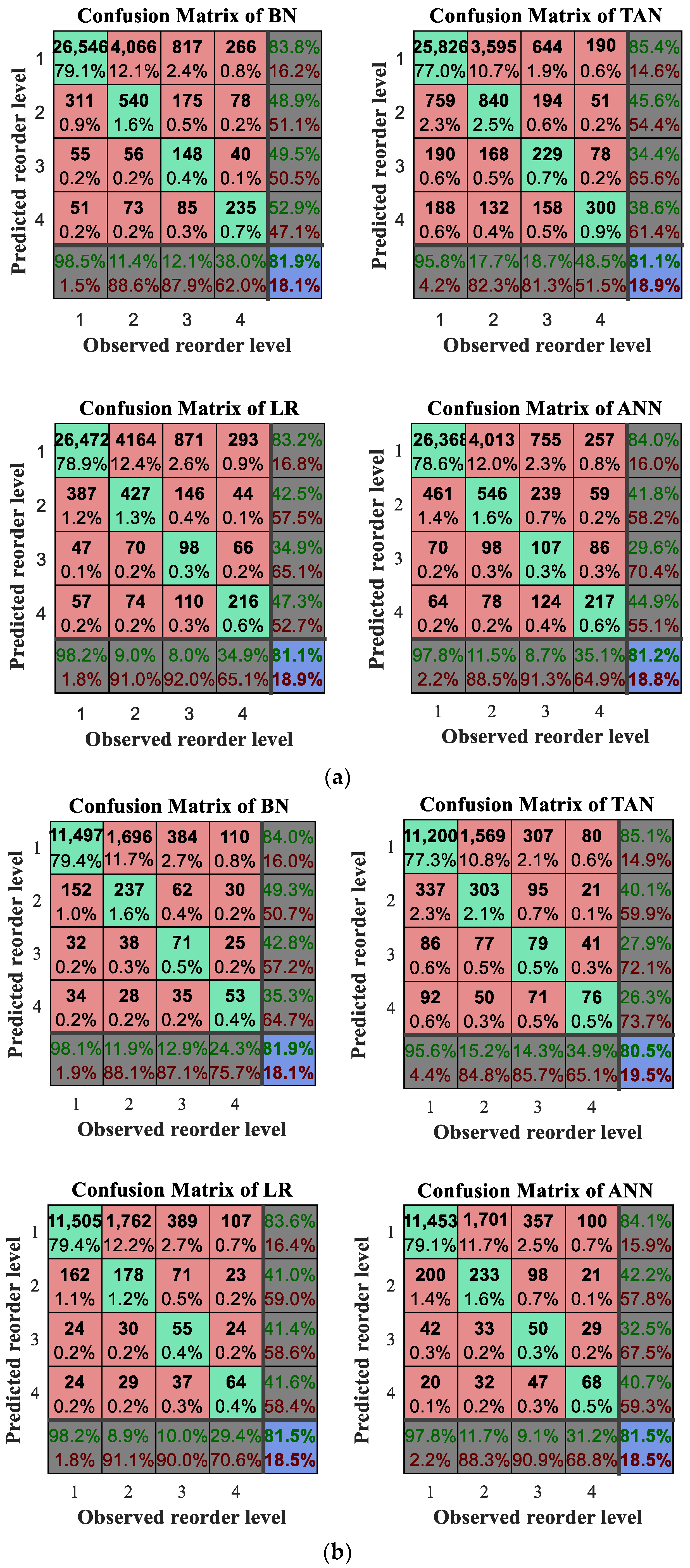
(1) Compute the posterior probability $P\left({\omega }_j|X\right)=P({\omega }_j)P(X|{\omega }_j)/{\displaystyle \sum _{j=1}^{4}P({\omega }_j)P(X|{\omega }_j)}$; (2) Compute $R\left({\alpha }_i|X\right)$ for the classification of ${\alpha }_i$ according to Equation (7); (3) Classify reorder level of $X$ to i with minimal $R\left({\alpha }_i|X\right)$, $i=1,2,3,4$ by Equation (8).

Initial results also show that the probability to predict order with an observed reorder level of 1 to 2, 3, and 4 decreases with an increase in the value of binned recency and the risk to predict the larger reorder level to the smaller one will also decrease. Therefore, four loss matrices corresponding to the binned recency 1, 2–3, 4–5, and 6–10 were introduced for final classification based on Algorithm 4, in which the value in the upper half of the matrix decreases with an increase in the value of binned recency while the value in the lower half of the matrix increases with an increase in the value of binned recency. The values were set to 1 and 0 in the non-diagonal positions and diagonal position, respectively, when recency is 1. The other three matrices are shown in

Table 6. Loss matrix for different binned recency values.

Predicted Value	Overserved Value
	Recency = 2–3				Recency = 4–5				Recency = 6–10
	1	2	3	4	1	2	3	4	1	2	3	4
1	0	1.2	1.25	1.3	0	1.15	1.2	1.25	0	1.1	1.15	1.2
2	1.3	0	0.8	0.9	1.35	0	0.75	0.85	1.4	0	0.7	0.8
3	1.35	0.75	0	0.9	1.4	0.8	0	0.85	1.45	0.85	0	0.8
4	1.45	0.85	0.75	0	1.5	0.9	0.8	0	1.55	0.95	0.85	0

.

4. Model Evaluation

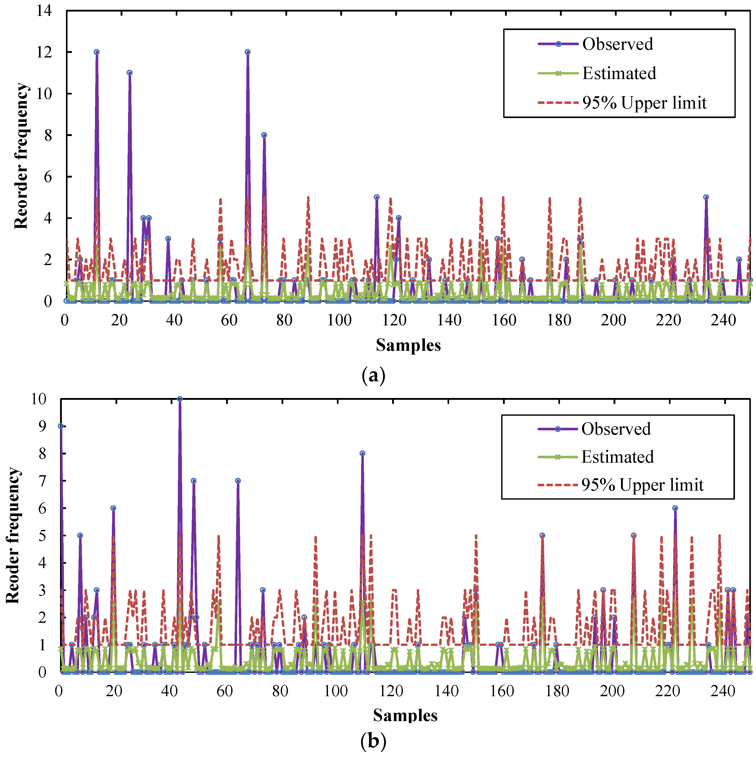
4.1. Estimation of Reorder Frequency

In order to get the expected reorder frequency for a given order, we use the sum of the mean value of reorder frequency in each level weighted by conditional probability as the expected reorder frequency. The expected output of the model can be computed by the equation below.

$$E(\mathrm{Re}Freq|Cluster=i)={\displaystyle \sum _{k=1}^{4}P(\mathrm{Re}l=k|Cluster=i)M(\mathrm{Re}l=k)},i=1,2,\dots .$$

(9)

where $M(\mathrm{Re}l=k)$ is the mean value of reorder frequency within six months for the samples with $\mathrm{Re}l=k$, which can be referred to

Table 7. Mean reorder frequency for different reorder levels.

Reorder Level	1	2	3	4
Mean value for training samples	0	1.28	3.67	10.03
Mean value for test samples	0	1.27	3.67	10.28
Mean value for all samples	0	1.28	3.67	10.09

. $P(\mathrm{Re}l=k|Cluster=i)$ is the average conditional probability determined by the modified BN with $\mathrm{Re}l=k$ given a specific cluster i and $Cluster=i$ represents the $i\mathrm{th}$ cluster of the samples determined by the clustering algorithm.

The purpose of the clustering is to classify samples according to their similarity by considering the input features of discretized F1–F7, Rec, and Ln. The k-summary approach that can handle both categorical and numerical data was adopted for the clustering and the number of clusters was set to 7 based on an initial experiment. On this basis, the average conditional probability of different reorder levels given different clusters is presented in

Table 8. Average conditional probability of different reorder levels given different clusters (%).

Reorder Level	Different Clusters
	C1	C2	C3	C4	C5	C6	C7
1	89.67	91.88	65.87	58.87	89.60	42.60	92.49
2	9.42	7.32	24.84	31.50	7.03	23.25	6.67
3	0.78	0.64	7.06	7.99	2.18	17.79	0.65
4	0.13	0.16	2.23	1.64	1.18	16.36	0.19

.

4.2. Evaluation Indicators

The confusion matrix was taken to visualize the performance of different approaches in which each column of the matrix represents the instances in an actual class while each row represents the instances in a predicted class. All correct predictions are located in the diagonal of each table and errors can be visually inspected by values outside the diagonal. Related terminology and derivations are defined in

Table 9. Terminology and derivations of the confusion matrix.

Terminology	Description
True positive (TP)	Number of correctly predicted instances for each column
False negative (FN)	Number of incorrectly predicted instances for each column
False positive (FP)	Number of incorrectly predicted instances for each row
True negative (TN)	Number of correctly predicted instances for each row
Sensitivity or true positive rate (TPR)	TP/(TP+FN)
False negative rate (FNR)	1-TPR
Specificity or true negative rate (TNR)	TN/(TN+FP)
False positive rate (FPR)	1-TNR
Positive predictive value (PPV)	TP/(TP+FP)
False discovery rate (FDR)	1-PPV
Accuracy (ACC)	(TP+TN)/Total instances

[33].

In order to evaluate the performance of the proposed model, the following mean squared error (MSE), mean absolute error (MAE), and mean absolute percentage error (MAPE) evaluation indicators were used. MSE is the average of square sums between the predicted reorder level ${\alpha }_i$ and the observed value ${\omega }_i$ [14]. It defines the goodness of fit of the models and is given by the following equation.

$$MSE=\frac{1}{n}{\displaystyle \sum _{i=1}^n{({\alpha }_i-{\omega }_i)}^2}$$

(10)

The MAE is the average of the sum of the absolute difference between observed values and the predicted reorder level, which can be expressed below.

$$MAE=\frac{1}{n}{\displaystyle \sum _{i=1}^n|({\alpha }_i-{\omega }_i)|}$$

(11)

The MAPE is the average of the sum of the normalized absolute difference between observed values and estimated values. The formula is written below.

$$MAPE=\frac{1}{n}{\displaystyle \sum _{i=1}^n|\frac{{\omega }_i-{\alpha }_i}{{\omega }_i}|\times 100}$$

(12)

4.3. Experimental Results

Reorder frequency of the samples six months after a set date can be taken as a random event for a manufacturer without prior knowledge and the models are expected to have errors in prediction. It is necessary for finding an upper limit and a lower limit to make as many as possible observed values lie in. Additionally, the small field data set may cause uncertain deviations between observed reorder levels and predicted ones. It is also impractical to fit the reorder frequency in a specific distribution absolutely. The counting nature of the reorder frequency makes it intuitive for using a Poisson distribution as the probability distribution function (PDF). Therefore, assuming the reorder frequency in each reorder level following a Poisson distribution is justifiable since it has a high repetition occurrence rate and more numbers under low reorder levels and a small probability at high reorder levels, which is shown in Table 2. The approximate upper limit for 95% confidence aligns with the Poisson cumulative distribution function (CDF) and is equal to or greater than 95%. The lower limits are considered to be zero because of the nonnegative counting property of Poisson distribution [14].

Monte Carlo simulation is used to weaken the influence of uncertainty factors in this research. It is an effective method for quantifying the variance resulting from the random nature of repetition events. For any sample (orders with the same production number) with a given cluster and the distribution of the reorder frequency, a random number can be generated through simulation to present the reorder frequency for this sample and the 95% confidence upper limit can be obtained. As a result, it is used to estimate reorder frequency and the 95% upper limit for each sample. Along with the increase in the number of simulations, the prediction accuracy will increase gradually. Therefore, it can quantify the variance resulting from the randomness of repetition events. A procedure of Monte Carlo simulation is described below (Algorithm 5).

Algorithm 5. Monte Carlo simulation of reorder times.

(1) Given a specific order, determine the cluster of the sample; (2) Determine the expected reorder frequency (within six months after a set date) as the parameter (lamda) of Poisson PDF and CDF for the sample according to Equation (9) based on Table 7 and Table 8; (3) Generate n (10,000 here) random number by Poisson PDF with lamda as its expectation and take the average result of the n random number as the simulated reorder frequency; (4) Determine the least integer for Poisson CDF being greater than 0.95 as the 95% upper limit of reorder frequency for the order.

A total of 250 randomly selected samples with Monte Carlo simulation results obtained by Algorithm 5 are presented in Figure 8. The performance of the Bayesian network for training and test data can be seen from Figure 8a,b, respectively. When the reorder level is low, the estimated value is close to the observed one. In some extreme situations, it can cause a greater reorder frequency than what can be predicted. The presentation in figures is that the observed values are higher than the 95% upper limits. Figure 8 indicates that the difference between estimated values and actual values is small in most cases and almost all of them are less than 1.

In order to verify the proposed ensemble approach in this research, the data preprocessing and modified BN prediction model were implemented and the performance was compared to other classifiers including TAN, AdaBoost, and ANN. Among the four competing methods, TAN as a naïve Bayesian network has been widely utilized in classification [17,18]. AdaBoost is an ensemble method whose output is the weighted average of many weak classifiers and is the best-known and most widely applied boosting algorithm in both research and practice [34]. ANN has a strong learning ability and has also been widely used for prediction and classification [35,36,37]. TAN and ANN were implemented in the IBM SPSS Modeler and AdaBoost was developed by Matlab while the proposed modified BN was developed based on Matlab and package FullBNT.

Confusion matrices of different approaches are given in Figure 9. These confusion matrices show that TAN achieved the highest sensitivity for observed reorder levels 2, 3, and 4. However, the ability to identify a reorder level 1 was weak and the unbalanced and biased distribution of reorder level 1 can greatly increase the production risk if a large amount of orders were taken as batch production in advance without customers’ confirmation. On the other hand, the modified BN achieved better results with sensitivity 98.5% and 98.1% for training and test samples, respectively. It can reduce the number of samples with a reorder level 1 to be incorrectly predicted as 2, 3, or 4, which reduces the risk of batch production. In addition, the modified BN can correctly identify a higher amount of orders with an observed reorder level 2 and 3 compared with AdaBoost and ANN both for training and test samples. The sensitivity of the modified BN for observed reorder level 4 deteriorated for the test sample. However, many samples have been predicted as 2 or 3, which can also be taken for batch production. Overall indicators of confusion matrices also show that the modified BN obtained the highest accuracy (81.9%) both for training and test samples.

The approaches were compared both for training and test samples according to indicators presented in Equations (10)–(12) and the comparison results can be referred to

Table 10. Comparison of classifiers according to different indicators.

Classifiers	Training Samples			Test Samples
	MSE	MAE	MAPE	MSE	MAE	MAPE
Modified BN	689.98	0.2306	10.6965	291.74	0.2239	11.0818
TAN	666.8964	0.2421	11.5641	302.2279	0.2509	11.9724
AdaBoost	738.0686	0.2407	11.2314	308.0735	0.2358	11.0472
ANN	692.7819	0.2349	11.3129	293.1946	0.2346	11.1991

. It shows that the proposed modified BN obtained the lowest MAE and MAPE for training samples and the lowest MSE and MAE for test samples. The results in Figure 9 also illustrate that TAN obtained the maximum correctly classified instances with observed reorder levels of 2, 3, and 4 as well as the maximum incorrectly classified instances with an observed reorder level of 1 compared to the other classifiers. Therefore, the indicators show that TAN achieved the lowest MSE for training samples as well as almost the largest MAE and MAPE both for training and test samples. This may be caused by redundant links between the evidence node and the missing strong links such as the causal relationships between F2, F3, F6, and F1. Yet, it is worth noting that TAN deteriorated greatly on the test dataset according to MAE and MAPE, which indicates that the TAN considered in the current study lacked robustness and generalization ability. The ANN exhibited steady performance both for training and test samples but had no superiority according to the three indicators. The AdaBoost achieved slightly better performance for test samples for the indicator MAPE but the worst performance for the indicators MSE and MAE.

The above results indicate that the modified BN combing CMI, LSP, and expert experience maintains the DAG requirement of BN and produces a more nuanced network that captures the main dependency relationships among evidence nodes (variables) while deleting some weak dependency relationships without allowing arbitrary graphical structures that would make it harder to interpret and extract relations to enhance the prediction model. At the same time, the conditional expected loss can benefit the final classification and it can exhibit better performance especially when compared to TAN. In addition, the modified BN has the clearest common sense interpretation.

5. Conclusions

In this paper, the identification of repeated PCB orders for batch production was transformed into a reorder level prediction problem and a modified Bayesian network model with Monte Carlo simulations to study the relationship between different characteristic variables and reorder levels of PCB within six months was established. Reorder frequency was divided into four reorder levels and variables related to a reorder level were specified. Field data was exported and integrated from a PCB manufacturer with 33,542 training samples and 14,484 test samples. Normalization and PCA were employed to reduce differences and redundancy of the datasets, respectively. PCA results indicated that the causes of the reorder level are closely related to seven principal components and the other two variables, i.e., recency and layer number. Entropy minimization based binning method was employed to discretize model variables for the purpose of reducing input type and capturing better performance and results. The modified structure of BN was established by deleting redundant connections between nodes (with weak link strength) and corresponding conditional probability tables based on conditional mutual information and link strength percentage combining with expert experience. This can facilitate the manufacturer to comprehend causal interactions between variables. On this basis, the conditional expected loss was presented for final classification considering different misclassification risk.

Monte Carlo simulation was conducted to enable the determination with greater accuracy of a mean and confidence interval for reorder frequency estimations based on the predicted reorder level. The upper limits of reorder frequency are particularly useful for the PCB manufacturer as a basis of each reorder level. The performance of the proposed modified BN was visualized by confusion matrix, evaluated by three indicators, and compared to three advanced methods including TAN, AdaBoost, and ANN. It was found that the modified BN prediction model achieved steady and satisfactory results both for training and test samples with the clearest common sense interpretation. Therefore, the proposed model in this paper is an effective approach to capture the repetition pattern of PCB orders that have seldom been studied before. The established explicit relationship between the variables including extracted factors and the reorder level by the causal network can directly facilitate order selection for batch production that can be conducted according to the decision making step given in Figure 1.

The main contributions of this work are summarized below.

• The tricky problem of identifying repeated orders for batch production was transformed into a reorder level prediction problem and then a reorder level prediction model based on modified causal Bayesian network was proposed. From the historically accumulated data in a PCB manufacturer, different characteristic variables were extracted and specified for the model.
• PCA was employed for data compression and factors extraction. Yet, an entropy minimization based method was presented to discretize variable and extracted factors. They could facilitate data compression, input type reduction, and better classification performance.
• In order to avoid the defect of TAN BN that easily misses strong links between nodes and generates redundant weak links, CMI and LSP were combined for the establishment of the BN structure.
• By using Monte Carlo simulations, the confidence upper limits of reorder frequency within six months were determined and the influence of the random nature of reorder was reduced.

Further research will be made to design intelligent approaches that can predict and determine reasonable batch production area for each candidate order. Further attempts will also be made to apply this method to similar order-oriented production and develop other intelligent techniques for the repetition pattern excavation.

References

1. Marques, A.C.; Cabrera, C.J.; Malfatti, C.F. Printed circuit boards: A review on the perspective of sustainability. J. Environ. Manag. 2013, 131, 298–306. [Google Scholar] [CrossRef] [PubMed]
2. Ngai, E.W.T.; Xiu, L.; Chau, D.C.K. Application of data mining techniques in customer relationship management: A literature review and classification. Exp. Syst. Appl. 2009, 36, 2592–2602. [Google Scholar] [CrossRef]
3. Dursun, A.; Caber, M. Using data mining techniques for profiling profitable hotel customers: An application of RFM analysis. Tour. Manag. Perspect. 2016, 18, 153–160. [Google Scholar] [CrossRef]
4. Chen, Y.L.; Kuo, M.H.; Wu, S.Y.; Tang, K. Discovering recency, frequency, and monetary (RFM) sequential patterns from customers’ purchasing data. Electron. Commer. Res. Appl. 2009, 8, 241–251. [Google Scholar] [CrossRef]
5. Hu, Y.; Yeh, T. Discovering valuable frequent patterns based on RFM analysis without customer identification information. Knowl. Syst. 2014, 61, 76–88. [Google Scholar] [CrossRef]
6. Coussement, K.; Filip, A.M.V.B.; Bock, K.W. Dataac accuracy’s impt on segmentation performance: Benchmarking RFM analysis, logistic regression, and decision trees. J. Bus. Res. 2014, 67, 2751–2758. [Google Scholar] [CrossRef]
7. Mohammadzadeh, M.; Hoseini, Z.Z.; Derafshi, H. A data mining approach for modeling churn behavior via RFM model in specialized clinics case study: A public sector hospital in Tehran. Procedia Comput. Sci. 2017, 120, 23–30. [Google Scholar] [CrossRef]
8. Song, M.N.; Zhao, X.J.; Haihong, E.; Qu, Z.H. Statistics-based CRM approach via time series segmenting RFM on large scale data. Knowl. Syst. 2017, 132, 21–29. [Google Scholar] [CrossRef]
9. Liu, J. Using big data database to construct new GFuzzy text mining and decision algorithm for targeting and classifying customers. Comput. Ind. Eng. 2018. [Google Scholar] [CrossRef]
10. Sarti, S.; Darnall, N.; Testa, F. Market segmentation of consumers based on their actual sustainability and health-related purchases. J. Clean. Prod. 2018, 192, 270–280. [Google Scholar] [CrossRef]
11. Murray, P.W.; Agard, B.; Barajas, M.A. Forecast of individual customer’s demand from a large and noisy dataset. Comput. Ind. Eng. 2018, 118, 33–43. [Google Scholar] [CrossRef]
12. De Caigny, A.; Coussement, K.; Bock, K.W.D. A new hybrid classification algorithm for customer churn prediction based on logistic regression and decision trees. Eur. J. Oper. Res. 2018, 269, 760–772. [Google Scholar] [CrossRef]
13. Zerbino, P.; Aloini, D.; Dulmin, R.; Mininno, V. Big Data-enabled customer relationship management: A holistic approach. Inform. Proc. Manag. 2018. [Google Scholar] [CrossRef]
14. Wang, G.; Xu, T.H.; Tang, T.; Yuan, T.M.; Wang, H.F. A Bayesian network model for prediction of weather-related failures in railway turnout systems. Expert Syst. Appl. 2017, 69, 247–256. [Google Scholar] [CrossRef]
15. Arias, J.; Gamez, J.A.; Puerta, J.M. Learning distributed discrete Bayesian network classifiers under MapReduce with Apache Spark. Knowl. Based Syst. 2017, 11, 16–26. [Google Scholar] [CrossRef]
16. Thorson, J.T.; Johnson, K.F.; Methot, R.D.; Taylor, I.G. Model-based estimates of effective sample size in stock assessment models using the Dirichlet-multinomial distribution. Fish. Res. 2017, 192, 84–93. [Google Scholar] [CrossRef]
17. Mack, D.L.C.; Biswas, G.; Koutsoukos, X.D.; Mylaraswamy, D. Learning Bayesian network structures to augment aircraft diagnostic reference models. IEEE Trans. Autom. Sci. Eng. 2017, 14, 358–369. [Google Scholar] [CrossRef]
18. Alonso-Montesinos, J.; Martínez-Durbán, M.; Sagrado, J.; Águila, I.M.D.; Batlles, F.J. The application of Bayesian network classifiers to cloud classification in satellite images. Renew. Energy 2016, 97, 155–161. [Google Scholar] [CrossRef]
19. Hosseini, S.; Barker, K. Modeling infrastructure resilience using Bayesian networks: A case study of inland waterway ports. Comput. Ind. Eng. 2016, 93, 252–266. [Google Scholar] [CrossRef]
20. Hosseini, S.; Barker, K. A Bayesian network model for resilience-based supplier selection. Int. J. Prod. Econ. 2016, 180, 68–87. [Google Scholar] [CrossRef]
21. Li, B.C.; Yang, Y.L. Complexity of concept classes induced by discrete Markov networks and Bayesian networks. Pattern Recognit. 2018. [Google Scholar] [CrossRef]
22. Liu, B.; Hu, J.; Yan, F.; Turkson, R.F.; Lin, F. A novel optimal support vector machine ensemble model for NOx emissions prediction of a diesel engine. Measurement 2016, 92, 183–192. [Google Scholar] [CrossRef]
23. Ramrez-Gallego, S.; Krawczyk, B.; Woniak, M.; Woniak, M.; Herrera, F. A survey on data preprocessing for data stream mining: Current status and future directions. Neurocomputing 2017, 239, 39–57. [Google Scholar] [CrossRef]
24. Fayyad, U.; Irani, K. Multi-interval discretization of continuous-valued attributes for classification learning. Int. J. Conf. Artif. Intel. 1993, 1022–1029. [Google Scholar]
25. Boonchuay, K.; Sinapiromsaran, K.; Lursinsap, C. Decision tree induction based on minority entropy for the class imbalance problem. Pattern Anal. Appl. 2017, 20, 769–782. [Google Scholar] [CrossRef]
26. Tahan, M.H.; Asadi, S. MEMOD: A novel multivariate evolutionary multi-objective discretization. Soft Comput. 2017, 22, 1–23. [Google Scholar] [CrossRef]
27. Zhao, Y.; Xiao, F.; Wang, S. An intelligent chiller fault detection and diagnosis methodology using bayesian belief network. Energy Build. 2013, 57, 278–288. [Google Scholar] [CrossRef]
28. Jun, H.B.; Kim, D. A Bayesian network-based approach for fault analysis. Expert Syst. Appl. 2017, 81, 332–348. [Google Scholar] [CrossRef]
29. Wang, S.C.; Gao, R.; Wang, L.M. Bayesian network classifiers based on Gaussian kernel density. Expert Syst. Appl. 2016, 51, 207–217. [Google Scholar] [CrossRef]
30. Gan, H.X.; Zhang, Y.; Song, Q. Bayesian belief network for positive unlabeled learning with uncertainty. Pattern Recogn. Lett. 2017, 90, 28–35. [Google Scholar] [CrossRef]
31. Friedman, N.; Geiger, D.; Goldszmidt, M. Bayesian network classifiers. Mach. Learn. 1997, 29, 131–163. [Google Scholar] [CrossRef]
32. Imme, E.U. Georgia Tech Research Report: Tutorial on How to Measure Link Strengths in Discrete Bayesian Networks; Woodruff School of Mechanical Engineering, Georgia Institute of Technology: Atlanta, GA, USA, 2009. [Google Scholar]
33. Confusion Matrix. Available online: https://en.wikipedia.org/wiki/Confusion_matrix (accessed on 11 October 2017).
34. Liu, H.; Tian, H.Q.; Li, Y.F.; Zhang, L. Comparison of four Adaboost algorithm based artificial neural networks in wind speed predictions. Energy Convers. Manag. 2015, 92, 67–81. [Google Scholar] [CrossRef]
35. Cortes, C.; Gonzalvo, X.; Kuznetsov, V.; Mohri, M.; Yang, S. AdaNet: Adaptive structural learning of artificial neural networks. arXiv, 2016; arXiv:1607.01097. [Google Scholar]
36. Sharma, A.; Sahoo, P.K.; Tripathi, R.K.; Meher, L.C. Artificial neural network-based prediction of performance and emission characteristics of CI engine using polanga as a biodiese. Int. J. Ambient Energy 2016, 37, 559–570. [Google Scholar] [CrossRef]
37. Saravanan, K.; Sasithra, S. Review on classification based on artificial neural networks. Int J. Ambient Syst. Appl. 2014, 2, 11–18. [Google Scholar]
Figure 1. The framework of the reorder level prediction for batch production.
Applsci 08 00915 g001
Figure 2. Variance explained based on principal component analysis.
Applsci 08 00915 g002
Figure 3. Component matrix.
Applsci 08 00915 g003
Figure 4. Proportions of different reorder level in different binned intervals.
Applsci 08 00915 g004
Figure 5. Bayesian network structure with entropy information and link strength percentage.
Applsci 08 00915 g005
Figure 6. Posterior probabilities corresponding to different predicted reorder levels.
Applsci 08 00915 g006
Figure 7. Posterior probabilities for 100 randomly selected samples. (a) Posterior probabilities for 100 randomly selected samples with observed Rel = 2. (b) Posterior probabilities for 100 randomly selected samples with observed Rel = 4.
Applsci 08 00915 g007
Figure 8. Observed and estimated reorder frequency with 95% upper limits by Monte Carlo simulations. (a) Training observed and estimated reorder frequency with 95% upper limits. (b) Test observed and estimated reorder frequency with 95% upper limits.
Applsci 08 00915 g008
Figure 9. Confusion matrix of different approaches. (a) Confusion matrix of different methods for training samples. (b) Confusion matrix of different methods for test samples.
Applsci 08 00915 g009