Efficient Implementations of Four-Dimensional GLV-GLS Scalar Multiplication on 8-Bit, 16-Bit, and 32-Bit Microcontrollers

Abstract

In this paper, we present the first constant-time implementations of four-dimensional Gallant–Lambert–Vanstone and Galbraith–Lin–Scott (GLV-GLS) scalar multiplication using curve $\mathtt{Ted}\mathtt{127}$-$\mathtt{glv}\mathtt{4}$ on 8-bit AVR, 16-bit MSP430, and 32-bit ARM processors. In Asiacrypt 2012, Longa and Sica introduced the four-dimensional GLV-GLS scalar multiplication, and they reported the implementation results on Intel processors. However, they did not consider efficient implementations on resource-constrained embedded devices. We have optimized the performance of scalar multiplication using curve $\mathtt{Ted}\mathtt{127}$-$\mathtt{glv}\mathtt{4}$ on 8-bit AVR, 16-bit MSP430, and 32-bit ARM processors. Our implementations compute a variable-base scalar multiplication in 6,856,026, 4,158,453, and 447,836 cycles on AVR, MSP430, and ARM Cortex-M4 processors, respectively. Recently, Four$\mathbb{Q}$-based scalar multiplication has provided the fastest implementation results on AVR, MSP430, and ARM Cortex-M4 processors to date. Compared to Four$\mathbb{Q}$-based scalar multiplication, the proposed implementations require 4.49% more computational cost on AVR, but save 2.85% and 4.61% cycles on MSP430 and ARM, respectively. Our 16-bit and 32-bit implementation results set new speed records for variable-base scalar multiplication.

1. Introduction

Wireless sensor networks (WSNs) are wireless networks consisting of a large number of resource-constrained sensor nodes, where each node is equipped with a sensor to monitor physical phenomena, such as temperature, light, and pressure. The main features of WSNs are resource constraints, such as storage, computing power, and sensing distance. Recently, the energy consumption of data centers has attracted attention because of the fast growth of data throughput. WSNs can provide a solution for data collection and data processing in various applications including data center monitoring. That is, WSNs can be utilized for data center monitoring to improve the efficiency of energy consumption. Several solutions were proposed to solve this problem [1,2].

Since sensor nodes are usually deployed in remote areas and left unattended, they can be led to network security issues, such as node capture, eavesdropping, and message tampering during data communication. Additionally, many application areas of WSNs require data confidentiality, integrity, authentication, and non-repudiation, meaning there is a need for an efficient cryptographic mechanism to satisfy current security requirements. However, due to the constraint of WSNs, it is difficult to utilize the conventional cryptographic algorithms. Therefore, efficient cryptographic algorithms considering code size, computation time, and power consumption are required for the security of WSNs.

In 1985, elliptic curve cryptography (ECC) was proposed independently of public key cryptography (PKC) by Miller and Koblitz [3,4]. ECC is mainly used for digital signature and key exchange based on the elliptic curve discrete logarithm problem (ECDLP), which is defined by elliptic curve point operations in a finite field. ECC provides the same security level with a smaller key size compared to existing PKC algorithms such as Rivest-Shamir-Adleman (RSA) cryptosystem [5]. For example, ECC over ${\mathbb{F}}_p$ with a 256-bit prime p provides an equivalent security level as RSA using 3072-bit key. Because RSA uses a small integer as the public key, RSA public key operations can be efficiently computed. However, RSA private key operations are extremely slower than ECC, therefore they have limited use in the applications of WSNs. Therefore, ECC can be efficiently utilized than RSA for resource-constrained WSNs devices, such as smart cards and sensor nodes.

However, recently proposed manipulation and backdoors have raised the suspicion of weakness in previous ECC standards. In particular, the National Institute of Standards and Technology (NIST) P-224 curve is not secure against twist attacks, which are the combined attacks that use the small-subgroup attacks and the invalid-curve attacks using the twist of curve [6]. The dual elliptic curve deterministic random bit generator (Dual_EC_DRBG) is a pseudo-random number generator (PRNG) standardized in NIST SP 800-90A. However, the revised version of NIST SP 800-90A standard removes Dual_EC_DRBG because this algorithm contains a backdoor for the national security agency (NSA) [7].

Therefore, the demand for next generation elliptic curves has increased. Specific examples of such curves are Curve25519, Ed448-Goldilocks, and twisted Edwards curves [8,9,10]. The main features of these curves are the selection of efficient parameters. The Curve25519 utilizes a prime of the form $p=2^{255}-19$ and a fast Montgomery elliptic curve. The Ed448-Goldilocks curve utilizes a Solinas trinomial prime of the form $p=2^{448}-2^{224}-1$, which provides fast field arithmetic on both 32-bit and 64-bit machines because $224=28\times 8=32\times 7=56\times 4$. These parameters can accelerate the performance of ECC-based protocols. The details of the twisted Edwards curves can be found in Section 2.3.

Scalar multiplicationor point multiplication computes an operation $kP$ using an elliptic curve point P and a scalar k. This operation determines the performance of ECC. Therefore, many researchers have proposed various methods to improve the efficiency of scalar multiplication. The speed-up methods for scalar multiplication can be classified into three types: methods based on speeding up the finite field exponentiation, such as comb techniques and windowing methods, scalar recoding methods, and methods that are particular to elliptic curve scalar multiplication [11].

Speed-up methods using efficiently computable endomorphisms are one type of method that are particular to elliptic curve scalar multiplication. The Gallant–Lambert–Vanstone (GLV) method proposed by Gallant et al. is a method for accelerating scalar multiplication by using efficiently computable endomorphisms [11]. If the cost of computing endomorphism is less than (bit-length of curve order)/3 elliptic curve point doubling (ECDBL) operations, then this method has a computational advantage. Their method reduces about half of the ECDBL operations and saves the costs of scalar multiplication by roughly 33%. Additionally, recent studies have reported that scalar multiplication methods using efficiently computable endomorphisms are significantly faster than generalized methods. The Galbraith–Lin–Scott (GLS) curves proposed by Galbraith et al. constructed an efficiently computable endomorphism for elliptic curves defined over ${\mathbb{F}}_{p^2}$, where p is a prime number [12]. They demonstrated that the GLV method can efficiently compute scalar multiplication on such curves. Longa and Gebotys [13] presented an efficient implementation of two-dimensional GLS curves over ${\mathbb{F}}_{p^2}$.

In 2012, Longa and Sica [14] proposed four-dimensional GLV-GLS curves over ${\mathbb{F}}_{p^2}$, which generalized the GLV method and GLS curves. Hu et al. [15] proposed a GLV-GLS curve over ${\mathbb{F}}_{p^2}$, which supports the four-dimensional scalar decomposition. They reported the implementation results indicating that the four-dimensional GLV-GLS scalar multiplication reduces at most 22% of computational cost than the two-dimensional GLV method. Bos et al. [16] proposed two- and four-dimensional scalar decompositions over genus 2 curves defined over ${\mathbb{F}}_{p^2}$. Bos et al. [17] introduced an eight-dimensional GLV-GLS method over genus 2 curves defined over ${\mathbb{F}}_{p^2}$. Oliveira et al. [18] presented the implementation results of a two-dimensional GLV method over binary GLS elliptic curves defined over ${\mathbb{F}}_{2^{254}}$. Guillevic and Ionica [19] utilized the four-dimensional GLV method on genus 1 curves defined over ${\mathbb{F}}_{p^2}$ and genus 2 curves defined over ${\mathbb{F}}_p$. Smith [20] proposed a new family of elliptic curves over ${\mathbb{F}}_{p^2}$, called “$\mathbb{Q}$-curves”. Costello and Longa [21] introduced a four-dimensional $\mathbb{Q}$ curve defined over ${\mathbb{F}}_{p^2}$, called “Four$\mathbb{Q}$”. They reported the implementation results of Four$\mathbb{Q}$ on various Intel and AMD processors.

After a Four$\mathbb{Q}$-based approach has been proposed, many implementation results were reported considering various environments, such as AVR, MSP430, ARM, and field-programmable gate array (FPGA) devices [22,23,24]. An efficient Four$\mathbb{Q}$-based implementation on 32-bit ARM processor with the NEON single instruction multiple data (SIMD) instruction set was proposed by Longa [22]. Järvinen et al. [23] proposed a fast and compact Four$\mathbb{Q}$-based implementation on FPGA device. In CHES 2017, Liu et al. [24] presented highly optimized implementations using curve Four$\mathbb{Q}$ on 8-bit AVR, 16-bit MSP430, and 32-bit ARM Cortex-M4 processors, respectively.

In the case of curve $\mathtt{Ted}\mathtt{127}$-$\mathtt{glv}\mathtt{4}$, Longa and Sica and Faz-Hernández et al. [14,25] reported the implementation results on high-end processors, such as Intel Sandy Bridge, Intel Ivy Bridge, and ARM Cortex-A processors. However, efficient implementations on resource-constrained embedded devices have not been considered to date. Therefore, we focused on optimized implementations of scalar multiplication using curve $\mathtt{Ted}\mathtt{127}$-$\mathtt{glv}\mathtt{4}$ on 8-bit ATxmega256A3, 16-bit MSP430FR5969, and 32-bit ARM Cortex-M4 processors, respectively.

Our main contributions can be summarized as follows:

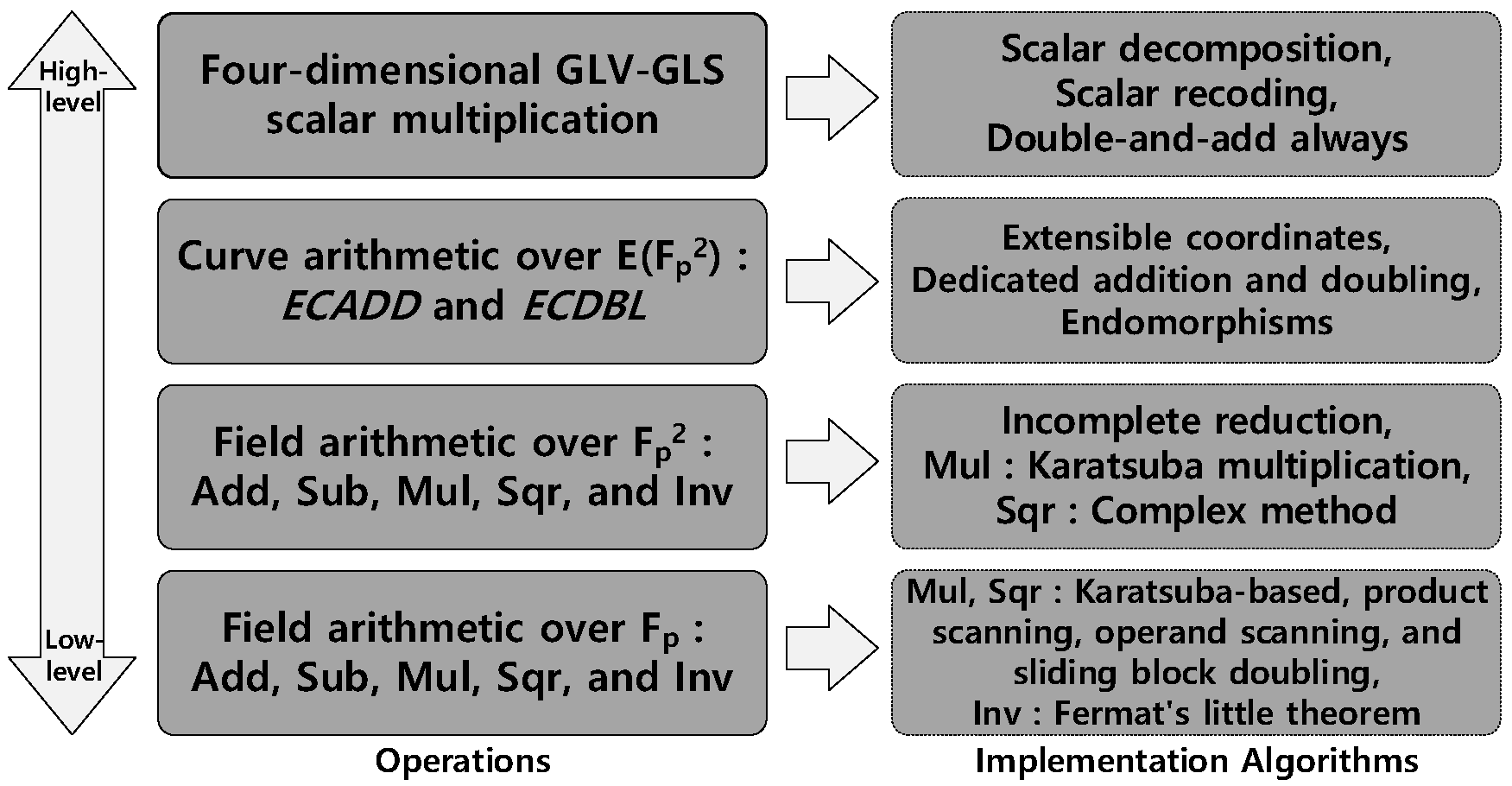
• We present efficient implementations at each level of the implementation hierarchy of four-dimensional GLV-GLS scalar multiplication considering the features of 8-bit AVR, 16-bit MSP430, and 32-bit ARM Cortex-M4 processors. To improve the performance of scalar multiplication, we carefully selected the internal algorithms at each level of the implementation hierarchy. These implementations also run in constant time to resist timing and cache-timing attacks [26,27].
• We demonstrate that the efficiently computable endomorphisms can accelerate the performance of four-dimensional GLV-GLS scalar multiplication. For this purpose, we analyze the operation counts of two elliptic curves “Ted127-glv4” and “Four$\mathbb{Q}$”, which support the four-dimensional GLV-GLS scalar multiplication. The GLV-GLS curve $\mathtt{Ted}\mathtt{127}$-$\mathtt{glv}\mathtt{4}$ requires fewer number of field arithmetic operations than Four$\mathbb{Q}$-based implementation to compute a single variable-base scalar multiplication. However, because Four$\mathbb{Q}$ uses a Mersenne prime $p=2^{127}-1$ and the curve $\mathtt{Ted}\mathtt{127}$-$\mathtt{glv}\mathtt{4}$ uses a Mersenne-like prime $p=2^{127}-5997$, Four$\mathbb{Q}$ has a computational advantage of faster field arithmetic operations. By using the computational advantage of endomorphisms, we overcome the computational disadvantage of curve $\mathtt{Ted}\mathtt{127}$-$\mathtt{glv}\mathtt{4}$ at field arithmetic level.
• We present the first constant-time implementations of four-dimensional GLV-GLS scalar multiplication using curve $\mathtt{Ted}\mathtt{127}$-$\mathtt{glv}\mathtt{4}$ on three target platforms, which have not been considered in previous works. The proposed implementations on AVR, MSP430, and ARM processors require 6,856,026, 4,158,453, and 447,836 cycles to compute a single variable-base scalar multiplication, respectively. Compared to Four$\mathbb{Q}$-based implementations [24], which have provided the fastest results to date, our results are 4.49% slower on AVR, but 2.85% and 4.61% faster on MSP430 and ARM, respectively. Our MSP430 and ARM implementations set new speed records for variable-base scalar multiplication.

The remainder of this paper is organized as follows. Section 2 describes preliminaries regarding ECC and its speed-up techniques, including the GLV and GLS methods. Section 3 presents a review of four-dimensional GLV-GLS scalar multiplication and its implementation hierarchy. Section 4 describes the implementation details of field arithmetic and optimization methods for the target platforms. Section 5 describes optimization methods for ECC in terms of point arithmetic and scalar multiplication. Experimental results and a comparison of our work to previous ECC implementations on AVR, MSP430, and ARM processors are presented in Section 6. Finally, we conclude this paper in Section 7.

2. Preliminaries

In Section 2.1, we describe the field representation and notations used for the remainder of this paper. We briefly describe ECC using a short Weierstrass curve and its group law in Section 2.2. We also describe twisted Edwards curves, which are the target of our implementation, in Section 2.3. In Section 2.4, we describe the GLV-GLS method including the GLV method and GLS curves.

2.1. Field Representation and Notations

We assume that the target platform has a w-bit architecture. Let $n=\lceil {log}_{2}p\rceil$ be the bit-length of a Mersenne-like prime $p=2^n-c$, where c is small. Let $m=\lceil n/w\rceil$ be its word-length. Then, an arbitrary element $a\in {\mathbb{F}}_p$ is represented by an array $(a_{m-1},\cdots ,a_2,a_1,a_0)$ of mw-bit words. The notations $M_1,S_1,I_1$, and $A_1$ represent multiplication, squaring, inversion, and addition (subtraction) over ${\mathbb{F}}_p$, respectively. Similarly, the notations $M_2,S_2,I_2$, and $A_2$ represent multiplication, squaring, inversion, and addition (subtraction) over ${\mathbb{F}}_{p^2}$, respectively. The notation $A_i$ represents multi-precision addition without modular reduction and the notation $M_d$ represents multiplication with a curve parameter.

2.2. Elliptic Curve Cryptography

Let ${\mathbb{F}}_q$ be a finite field with odd characteristic. An elliptic curve E over ${\mathbb{F}}_q$ is defined by a short Weierstrass equation of the following form:

$$\begin{array}{c}\hfill E:y^2=x^3+ax+b,\end{array}$$

where $a,b\in {\mathbb{F}}_q$ and $4a^3+27b^2\ne 0$.

Because the most important operation in ECC is scalar multiplication $kP$, it must be implemented efficiently. The basic method for computing $kP$ is comprised of two elliptic curve operations: elliptic curve point addition (ECADD) and the ECDBL operations. Let $P=(x_1,y_1)$ and $Q=(x_2,y_2)$ be two points on an elliptic curve E. The ECADD and ECDBL operations can be computed in affine coordinates as follows:

$$\begin{array}{cc}\hfill x_3={\lambda }^2-x_1-x_2,& y_3=\lambda (x_1-x_3)-y_1,\hfill \\ \hfill \lambda =\frac{y_2-y_1}{x_2-x_1}\mathrm{if}P\ne Q,& \mathrm{and}\lambda =\frac{3x_1^2+a}{2y_1}\mathrm{if}P=Q.\hfill \end{array}$$

The ECADD and ECDBL operations are composed of finite field arithmetic operations, such as field addition, subtraction, multiplication, squaring, and inversion. Therefore, to improve the performance of scalar multiplication, the internal algorithms such as field and curve arithmetic operations should be efficiently implemented.

2.3. Twisted Edwards Curves

The Edwards curves are a normal form of elliptic curves introduced by Edwards [28]. Bernstein and Lange [29] introduced Edwards curves defined by $x^2+y^2=c^2(1+d{x}^2{y}^2)$, where $c,d\in {\mathbb{F}}_q$ with $cd(1-d{c}^4)\ne 0$. In 2007, Bernstein et al. [10] introduced twisted Edwards curves, which are a generalization of Edwards curves defined by

$$\begin{array}{c}\hfill E_{a,d}:a{x}^2+y^2=1+d{x}^2{y}^2,\end{array}$$

where $a,d\in {\mathbb{F}}_q$ with $ad(a-d)\ne 0$. The Edwards curves are a special case of twisted Edwards curves with $a=1$. The point $(0,1)$ is the identity element and the point $(0,-1)$ has order two. The point $(1,0)$ and $(-1,0)$ have order four. The negative of a point $P=(x_1,y_1)$ is $-P=(-x_1,y_1)$. The ECADD operation of two points $P=(x_1,y_1)$ and $Q=(x_2,y_2)$ on a twisted Edwards curve E is defined as follows:

$$\begin{array}{c}\hfill (x_1,y_1)+(x_2,y_2)=\left(\frac{x_1{y}_2+y_1{x}_2}{1+d{x}_1{y}_1{x}_2{y}_2},\frac{y_1{y}_2-a{x}_1{x}_2}{1-d{x}_1{y}_1{x}_2{y}_2}\right).\end{array}$$

Because the addition law is unified, it can be used for computing the ECDBL operation. Suppose that two points P and Q have an odd order. Then, the denominators of the addition formula $1+d{x}_1{y}_1{x}_2{y}_2$ and $1-d{x}_1{y}_1{x}_2{y}_2$ are nonzero. Therefore, the doubling formula can be obtained as follows:

$$\begin{array}{c}\hfill 2(x_1,y_1)=\left(\frac{2x_1{y}_1}{y_1^2+a{x}_1^2},\frac{y_1^2-a{x}_1^2}{2-y_1^2-a{x}_1^2}\right).\end{array}$$

Two relationships can be obtained by considering the curve equation: $a{x}_1^2+y_1^2=1+d{x}_1^2{y}_1^2$ and $a{x}_2^2+y_2^2=1+d{x}_2^2{y}_2^2$. After straightforward elimination, the curve parameters a and d can be represented by $x_1,x_2,y_1$, and $y_2$. Substitutions in the unified addition formula yield the addition formula as follows:

$$\begin{array}{c}\hfill (x_1,y_1)+(x_2,y_2)=\left(\frac{x_1{y}_1+x_2{y}_2}{y_1{y}_2+a{x}_1{x}_2},\frac{x_1{y}_1-x_2{y}_2}{x_1{y}_2-y_1{x}_2}\right).\end{array}$$

These addition and doubling formulas are used in the dedicated addition and doubling formulas described in Section 5. The features of these formulas are independent of the curve parameter d [30].

2.4. The GLV-GLS Method

We will now describe the GLV method to explain the GLV-GLS method. Let E be an elliptic curve defined over a finite field ${\mathbb{F}}_q$. An endomorphism $\varphi$ of E over ${\mathbb{F}}_q$ is a rational map $\varphi :E\to E$ such that $\varphi \left(\mathcal{O}\right)=\mathcal{O}$ and $\varphi \left(P\right)=\left(g\right(P),h(P\left)\right)$ for all points $P\in E$, where g and h are rational functions and $\mathcal{O}$ is a point at infinity. An endomorphism $\varphi$ is a group homomorphism, defined as

$$\begin{array}{c}\hfill \varphi (P_1+P_2)=\varphi \left(P_1\right)+\varphi \left(P_2\right)\mathrm{for}\mathrm{all}{P}_1,P_2\in E.\end{array}$$

Suppose that $\#E\left({\mathbb{F}}_q\right)$ contains a subgroup of order r and let $\varphi$ be an efficiently computable endomorphism on E such that $\varphi \left(P\right)=\lambda P$ for some $1\le \lambda \le r-1$. The GLV method computes the integers $k_0$ and $k_1$ such that $k=k_0+k_1\lambda$ mod r for scalar multiplication $kP$. Because

$$\begin{array}{cc}\hfill kP& =k_{0}P+k_1\lambda P\hfill \\ & =k_{0}P+k_1\varphi \left(P\right),\hfill \end{array}$$

scalar multiplication $kP$ can be computed by computing $\varphi \left(P\right)$ and then using multiple scalar multiplications [31]. This is because the multi-scalars $k_0$ and $k_1$ have approximately half the bit-length of the scalar k. The efficiency of the GLV method depends on scalar decomposition and the efficiency of computing endomorphism $\varphi$.

The main concept of the GLS curves is described as follows: Let $E^{\prime }/{\mathbb{F}}_{q^2}$ be the quadratic twists of $E/{\mathbb{F}}_{q^2}$ [12]. Let $\psi$ be the quadratic twist map and $\pi$ be the q-th Frobenius endomorphism. Then, we can obtain the efficiently computable endomorphism $\varphi =\psi \circ \pi \circ {\psi }^{-1}$, which satisfies the equation $X^2+1=0$ if $p\equiv 5(mod8)$. However, GLS curves only work for elliptic curves over ${\mathbb{F}}_{q^m}$ with $m>1$.

As mentioned in the introduction, the GLV-GLS method is the generalized method of the GLV method and GLS curves. Let $\varphi$ and $\psi$ be two efficiently computable endomorphisms over ${\mathbb{F}}_{p^2}$ and P be a point of prime order r. Then, the four-dimensional scalar multiplication $kP$ for any scalar $k\in [1,r]$ can be computed as follows:

$$\begin{array}{cc}\hfill kP=& k_{0}P+k_1\varphi \left(P\right)+k_2\psi \left(P\right)+k_3\psi \left(\varphi \left(P\right)\right),\hfill \end{array}$$

where ${max}_i\left(\right|k_i\left|\right)<C{r}^{1/4}$ for $0\le i\le 3$ and C is some explicit constant. The details of internal algorithms of the four-dimensional scalar multiplication can be found in Section 4 and Section 5.

3. Review of Four-Dimensional GLV-GLS Scalar Multiplication

The curve $\mathtt{Ted}\mathtt{127}$-$\mathtt{glv}\mathtt{4}$ was introduced by Longa and Sica [14]. It is based on twisted Edwards curves and has efficiently computable endomorphisms, which facilitates the four-dimensional GLV-GLS scalar multiplication. The parameters of curve $\mathtt{Ted}\mathtt{127}$-$\mathtt{glv}\mathtt{4}$ are as follows:

$$\begin{array}{c}\hfill E/{\mathbb{F}}_{p^2}:-x^2+y^2=1+d{x}^2{y}^2,\end{array}$$

where $d=170141183460469231731687303715884099728+116829086847165810221872975542241037773i$, $p=2^{127}-5997$ and $\#E\left({\mathbb{F}}_{p^2}\right)=8r$, where r is a 251-bit prime. Let ${\mathbb{F}}_{p^2}={\mathbb{F}}_p\left[i\right]/(i^2+1)$ and $u=1+i$ be a quadratic non-residue in ${\mathbb{F}}_{p^2}$. E is isomorphic to the Weierstrass curve $E^{\prime }/{\mathbb{F}}_{p^2}:y^2=x^3-15/2u^{2}x-7u^3$. The curve $\mathtt{Ted}\mathtt{127}$-$\mathtt{glv}\mathtt{4}$ contains two efficiently computable endomorphisms $\varphi$ and $\psi$ defined over ${\mathbb{F}}_{p^2}$ as follows:

$$\begin{array}{cc}\hfill \varphi (x,y)=& \left(-\frac{({\zeta }_8^3+2{\zeta }_8^2+{\zeta }_8)x{y}^2+({\zeta }_8^3-2{\zeta }_8^2+{\zeta }_8)x}{2y},\frac{({\zeta }_8^2-1)y^2+2{\zeta }_8^3-{\zeta }_8^2+1}{(2{\zeta }_8^3+{\zeta }_8^2-1)y^2-{\zeta }_8^2+1}\right),\hfill \end{array}$$

$$\begin{array}{c}\hfill \psi (x,y)=\left({\zeta }_8{x}^p,\frac{1}{y^p}\right),\end{array}$$

where ${\zeta }_8=u/\sqrt{2}$ is a primitive eighth root of unity. It can be verified that ${\varphi }^2+2=0$ and ${\psi }^2+1=0$.

Let P be a point in $E/{\mathbb{F}}_{p^2}$ and k be a random scalar in the range $[1,r]$. Algorithm 1 outlines variable-base scalar multiplication using curve $\mathtt{Ted}\mathtt{127}$-$\mathtt{glv}\mathtt{4}$ and four-dimensional decompositions. Steps 1 and 2 in Algorithm 1 compute three endomorphisms $\varphi \left(P\right),\psi \left(P\right)$, and $\psi \left(\varphi \right(P\left)\right)$, and then compute the eight points $T\left[u\right]=P+u_0\varphi \left(P\right)+u_1\psi \left(P\right)+u_2\psi \left(\varphi \left(P\right)\right)$, where $u=(u_2,u_1,u_0)$ in $0\le u\le 7$. Step 3 decomposes the input scalar k into multi-scalars $(k_0,k_1,k_2,k_3)$ such that $0\le k_i\le 2^{65}$, where $0\le i\le 3$. For constant-time implementation, the multi-scalars $(k_0,k_1,k_2,k_3)$ must guarantee the same number of iterations of the main computation. Because all coordinates of scalar decomposition are less than $2^{65}$, we apply the scalar recoding algorithm to guarantee a fixed loop length for the main computation at step 4 [25]. The result of the scalar recoding is represented by 66 lookup table indices $d_i$ and 66 masks $m_i$, where $0\le i\le 65$. Steps 5 to 9 represent the main computation stage, including point loading, the ECADD operation, and the ECDBL operation. The result of the main computation is converted from an extensible coordinates to the affine coordinates in step 10. Therefore, a variable-base scalar multiplication using curve $\mathtt{Ted}\mathtt{127}$-$\mathtt{glv}\mathtt{4}$ requires one $\varphi \left(P\right)$ endomorphism, two $\psi \left(P\right)$ endomorphisms, and seven ECADD operations in the precomputation; 65 table lookups, 65 ECADD operations, and 65 ECDBL operations in the main computation; and one inversion and two field multiplications over ${\mathbb{F}}_{p^2}$ for point normalization.

Figure 1 describes the implementation hierarchy of four-dimensional GLV-GLS scalar multiplication and its internal algorithms. Because the implementation algorithms at each level affect the performance of scalar multiplication, we carefully choose proper algorithms considering the features of AVR, MSP430, and ARM processors. Additionally, field arithmetic over ${\mathbb{F}}_{p^2}$ and curve arithmetic are comprised of field arithmetic over ${\mathbb{F}}_p$, which is the computationally primary operations. Therefore, field arithmetic over ${\mathbb{F}}_p$ is written at the assembly level.

Figure 1. The implementation hierarchy of four-dimensional Gallant-Lambert-Vanstone and Galbraith-Lin-Scott (GLV-GLS) scalar multiplication.

Algorithm 1: Scalar multiplication using curve $\mathtt{Ted}\mathtt{127}$-$\mathtt{glv}\mathtt{4}$ [21].

Require:  Scalar $k\in [1,r]$ and point $P\in E/{\mathbb{F}}_{p^2}$. Ensure:  $kP$.  1: Compute $\varphi \left(P\right),\psi \left(P\right)$, and $\psi \left(\varphi \right(P\left)\right)$.  2: Compute $T\left[u\right]=P+u_0\varphi \left(P\right)+u_1\psi \left(P\right)+u_2\psi \left(\varphi \left(P\right)\right)$ where $u=(u_2,u_1,u_0)$ in $0\le u\le 7$.  3: Decompose the scalar k into the multi-scalars $(k_0,k_1,k_2,k_3)$.  4: Recode the multi-scalars $(k_0,k_1,k_2,k_3)$ to $(d_{65},\dots ,d_0)$ and $(m_{65},\dots ,m_0)$. $s_i=1$ if $m_i=-1$ and $s_i=-1$ if $m_i=0$.  5: $Q=s_{65}·T\left[d_{65}\right]$.  6: for$i=64$ to 0 do  7:  $Q\leftarrow 2Q$.  8:  $Q\leftarrow Q+s_i·T\left[d_i\right]$.  9: end for   10: returnQ.

4. Implementation Details of Field Arithmetic

In this section, we describe the implementation details of field arithmetic on AVR, MSP430X, and ARM Cortex-M4 processors using a Mersenne-like prime of the form $p=2^{127}-5997$. We describe the field arithmetic algorithms that are commonly used in three target platforms in Section 4.1, Section 4.2, Section 4.3 and Section 4.4. In Section 4.5, Section 4.6 and Section 4.7, we describe our optimization strategy for field arithmetic on AVR, MSP430, and ARM processors, respectively.

4.1. Field Addition and Subtraction over ${\mathbb{F}}_p$

The curve $\mathtt{Ted}\mathtt{127}$-$\mathtt{glv}\mathtt{4}$ uses a Mersenne-like prime of the form $p=2^{127}-5997$. An efficient field addition/subtraction method for this scenario was proposed by Bos et al. [16]. Let $0\le a,b<p=2^{127}-5997$. Field addition over ${\mathbb{F}}_p$ can be computed by $c=a+b(modp)=((a+5997)+b)-carry·2^{127}-(1-carry)·5997$, where $carry=0$ if $a+b+5997<2^{127}$. Otherwise, $carry=1$. The result is bounded by p because, if $a+b+5997<2^{127}$, then $a+b<2^{127}-5997$, whereas if $a+b+5997\ge 2^{127}$, then $(a+b+5997)(mod{2}^{127})=a+b-p<p$. Because $a+5997<2^{127}$, addition does not require carry propagation. Note that subtraction with $carry·2^{127}$ can be efficiently implemented by clearing the 128-th bit of $(a+5997)+b$.

Similar to field addition, field subtraction over ${\mathbb{F}}_p$ can be computed by $c=a-b(modp)=(a-b)+borrow·2^{127}-borrow·5997$, where $borrow=0$ if $a\ge b$, otherwise, $borrow=1$. Addition with $borrow·2^{127}$ can be implemented by clearing the 128-th bit of $a-b$.

4.2. Modular Reduction

To use primes of a special form may result in a faster reduction method [31]. The NIST recommends five primes for the elliptic curve digital signature algorithm (ECDSA). These primes can be represented as the sums or differences of powers of two and facilitate the fast reduction method. The curve $\mathtt{Ted}\mathtt{127}$-$\mathtt{glv}\mathtt{4}$ uses a Mersenne-like prime of the form $p=2^{127}-5997$. Therefore, modular reduction can be efficiently computed by using a NIST-like reduction method [16]. Let $0\le a,b\le p=2^{127}-5997$. We compute $c=a·b=2^{128}{c}_h+c_l$, where $0\le c_h,c_l<2^{128}$. The first reduction step can be computed by $c^{\prime }\equiv c_l+2·5997·c_h$. Then, the second reduction step can be computed by $c^{\prime }\equiv 2^{127}{R}_h+R_l\equiv R_l+5997·R_h(modp)$, where $R_l,5997·R_h<2^{127}$.

4.3. Inversion over ${\mathbb{F}}_p$

For the field inversion $a^{-1}(modp)$, we use the fact that $a^{-1}=a^{p-2}(modp)$ in Fermat’s little theorem (in our case, $a^{p-2}(modp)=a^{2^{127}-5999}(modp)$). This method can be implemented by modular exponentiation using fixed addition chains and guarantees constant-time execution requiring $13M_1+126S_1$ operations.

4.4. Field Arithmetic over ${\mathbb{F}}_{p^2}$

The incomplete reduction method proposed by Yanık et al. [32] is one of the optimization methods in field arithmetic over ${\mathbb{F}}_{p^2}$. Given two elements $a,b\in [0,p-1]$, the result of operations stays in the range $[0,2^m-1]$, where $p<2^m<2p-1$ and m is a fixed integer (in our case, $m=128$). Because the modulus of curve $\mathtt{Ted}\mathtt{127}$-$\mathtt{glv}\mathtt{4}$ is a Mersenne-like prime of the form $p=2^{127}-5997$, the incomplete reduction method can be applied more advantageously.

Let $a=a_0+a_{1}i$ and $b=b_0+b_{1}i$ be two arbitrary elements in a finite field ${\mathbb{F}}_{p^2}$. Field addition and subtraction over ${\mathbb{F}}_{p^2}$ can be computed by $a+b=(a_0+b_0)+(a_1+b_1)i$ and $a-b=(a_0-b_0)+(a_1-b_1)i$, respectively. Field inversion over ${\mathbb{F}}_{p^2}$ can be computed by $a^{-1}=(a_0-a_{1}i)/(a_0^2+a_1^2)$.

We utilize Karatsuba multiplication to compute field multiplication over ${\mathbb{F}}_{p^2}$. The Karatsuba multiplication uses the fact that $a·b=(a_0+a_{1}i)(b_0+b_{1}i)=(a_0{b}_0-a_1{b}_1)+\{(a_0+a_1)(b_0+b_1)-a_0{b}_0-a_1{b}_1\}i$, which can be computed by $3M_1+3A_1+2A_i$ operations. It requires $1A_1+2A_i$ more operations but saves 1$M_1$ operations compared to general multiplication methods, which require $4M_1+2A_1$ operations. Because field multiplication requires more computational cost than the multi-precision addition and field addition, the Karatsuba multiplication has a computational advantage. Algorithm 2 describes field multiplication over ${\mathbb{F}}_{p^2}$ using the Karatsuba multiplication and the incomplete reduction  method.

Algorithm 3 describes field squaring over ${\mathbb{F}}_{p^2}$ using the incomplete reduction method. Note that $a^2=(a_0^2-a_1^2)+2a_0{a}_{1}i=(a_0+a_1)(a_0-a_1)+2a_0{a}_{1}i$. The first representation can be computed by $1M_1+2S_1+1A_1+1A_i$ operations, and the remaining representation can be computed by $2M_1+1A_1+2A_i$ operations. Because $1M_1$ operation can be implemented faster than $2S_2$ operations, we use $2M_1+1A_1+2A_i$ operations to compute field squaring over ${\mathbb{F}}_{p^2}$. The results of steps 3 and 4 in Algorithm 2 and steps 1 and 3 in Algorithm 3 were represented by the incompletely reduced form.

Algorithm 2: Field multiplication over ${\mathbb{F}}_{p^2}$ [25].

Require:  $a=a_0+a_{1}i,b=b_0+b_{1}i\in {\mathbb{F}}_{p^2}$, $p=2^{127}-5997$. Ensure:  $c=a·b=c_0+c_{1}i\in {\mathbb{F}}_{p^2}$.  1: $t_1\leftarrow a_0\times b_0(modp)$ {$M_1$}  2: $t_2\leftarrow a_1\times b_1(modp)$ {$M_1$}  3: $t_3\leftarrow a_0+a_1$ {$A_i$}  4: $c_1\leftarrow b_0+b_1$ {$A_i$}  5: $c_1\leftarrow c_1\times t_3(modp)$ {$M_1$}  6: $c_1\leftarrow c_1-t_1(modp)$ {$A_1$}  7: $c_1\leftarrow c_1-t_2(modp)$ {$A_1$}  8: $c_0\leftarrow t_1-t_2(modp)$ {$A_1$}  9: returnc.

Algorithm 3: Field squaring over ${\mathbb{F}}_{p^2}$ [25].

Require:  $a=a_0+a_{1}i\in {\mathbb{F}}_{p^2}$, $p=2^{127}-5997$. Ensure:  $c=a^2=c_0+c_{1}i\in {\mathbb{F}}_{p^2}$.  1: $t_1\leftarrow a_0+a_1$ {$A_i$}  2: $t_2\leftarrow a_0-a_1(modp)$ {$A_1$}  3: $t_3\leftarrow a_0+a_0$ {$A_i$}  4: $c_0\leftarrow t_1\times t_2(modp)$ {$M_1$}  5: $c_1\leftarrow t_3\times a_1(modp)$ {$M_1$}  6: returnc.

4.5. Optimization Strategy on 8-Bit AVR

The AVR processor is a family of 8-bit microcontrollers that is widely used in MICA2/MICAz sensor motes. The AVR processors are equipped with an 8-bit integer multiplier and register file with 32×8-bit general registers that are numbered from $\mathtt{R}\mathtt{0}$ to $\mathtt{R}\mathtt{31}$. Registers $\mathtt{R}\mathtt{26}:\mathtt{R}\mathtt{27}$, $\mathtt{R}\mathtt{28}:\mathtt{R}\mathtt{29}$, and $\mathtt{R}\mathtt{30}:\mathtt{R}\mathtt{31}$ pairs are used as 16-bit indirect address registers called $\mathtt{X}$, $\mathtt{Y}$, and $\mathtt{Z}$. The automatic increment and decrement addressing modes are supported on all $\mathtt{X}$, $\mathtt{Y}$, and $\mathtt{Z}$ registers, and $\mathtt{Y}$ and $\mathtt{Z}$ support fixed positive displacement. $\mathtt{R}\mathtt{0}$ and $\mathtt{R}\mathtt{1}$ registers store the 16-bit results of $8\times 8$-bit multiplication. The AVR processors provide a typical 8-bit reduced instruction set computer (RISC) instruction set. The most important instructions for ECC are $8\times 8$-bit multiplication ($\mathtt{MUL}$) and memory access ($\mathtt{LD},\mathtt{ST}$) instructions, which require two cycles. Instructions between two registers, such as addition ($\mathtt{ADD},\mathtt{ADC}$) or subtraction ($\mathtt{SUB},\mathtt{SBC}$), require only one cycle. Therefore, the basic optimization strategy on 8-bit AVR is reducing the number of memory access instructions.

To simulate our implementations, we targeted the ATxmega256A3 processor [33]. This processor can be clocked up to 32 MHz and provides 256 KB of programmable flash memory, 16 KB of SRAM, and 4 KB of EEPROM.

Recently, Hutter and Schwabe [34] proposed a highly optimized Karatsuba multiplication for the 8-bit AVR processor. There are two variants of the Karatsuba multiplication method: the additive Karatsuba and subtractive Karatsuba methods. Algorithm 4 outlines the subtractive Karatsuba multiplication. We consider $n\times n$-bit multiplication, where n is even and $k=n/2$ (in our case, $n=128$ and $k=64$). The additive Karatsuba method can be computed similarly to Algorithm 4. However, the additive Karatsuba method may produce the carry bits in the addition of two numbers $(a_l+a_h)$ and $(b_l+b_h)$. The additional multiplication using the carry bits incurs a significant overhead for integer multiplication. The subtractive Karatsuba method does not produce carry bits in the computation of M, but computes two absolute values $|a_l-a_h|$ and $|b_l-b_h|$. This overhead is not only smaller than the overhead required for the  additive Karatsuba method, but can also be executed in constant-time. Therefore, we chose and implemented the subtractive Karatsuba multiplication for the 8-bit AVR implementation.

Algorithm 4: Subtractive Karatsuba multiplication [34].

Require:  $a=2^k{a}_h+a_l$, $b=2^k{b}_h+b_l\in {\mathbb{F}}_p$ for k-bit integers $a_l,a_h,b_l,$ and $b_h$. Ensure:  $c=a·b$.  1: Compute $L=a_l·b_l$  2: Compute $H=a_h·b_h$  3: Compute $M=|a_l-a_h|·|b_l-b_h|$  4: Set $t=0$, if $M=(a_l-a_h)·(b_l-b_h)$, $t=1$ otherwise  5: Compute $\widehat{M}={(-1)}^{t}M=(a_l-a_h)·(b_l-b_h)$  6: $c=A·B=L+2^k(L+H-\widehat{M})+2^{n}H$  7: returnc.

For integer squaring, we chose the sliding block doubling (SBD) method [35], which is more efficient than the subtractive Karatsuba method in the case of 128-bit operands on 8-bit AVR. To improve the performance of field arithmetic, we combined integer multiplication and squaring with modular reduction.

4.6. Optimization Strategy on 16-Bit MSP430X

The MSP430X processor was designed as an ultra-low power microcontroller based on the 16-bit RISC CPU. The MSP430X CPU has 16 20-bit registers that are numbered from $\mathtt{R}\mathtt{0}$ to $\mathtt{R}\mathtt{15}$. Registers $\mathtt{R}\mathtt{0}$ to $\mathtt{R}\mathtt{3}$ are special-purpose registers that are used as the program counter, stack pointer, status register, and constant generator, respectively. Registers $\mathtt{R}\mathtt{4}$ to $\mathtt{R}\mathtt{15}$ are general-purpose registers that are used to store data values, address pointers, and index values.

The MSP430X instruction set does not include multiply and multiply-and-accumulate (MAC) instructions. Instead, the MSP430 family is equipped with a memory-mapped hardware multiplier. The hardware multiplier provides four different multiply operations (unsigned multiplication, signed multiplication, unsigned multiplication and accumulation, and signed multiplication and accumulation) for the first operand, called $\mathtt{MPY},\mathtt{MPYS},\mathtt{MAC}$, and $\mathtt{MACS}$. The second operand register is common to all multiplier modes, called $\mathtt{OP}\mathtt{2}$. Namely, the first operand determines the operation type of the multiplier, but does not start the operation. Writing the second operand to the $\mathtt{OP}\mathtt{2}$ register starts the selected multiplication with two values. The multiplication result is written in three result registers $\mathtt{RESLO},\mathtt{RESHI}$, and $\mathtt{SUMEXT}$. $\mathtt{RESLO}$ stores the lower 16-bit of the result, $\mathtt{RESHI}$ stores the upper 16-bit of the result, and $\mathtt{SUMEXT}$ stores the carry bit or sign of the result.

The MSP430X processor provides seven addressing modes for the source operand and four addressing modes for the destination operand. The total computation time depends on the instruction format and the addressing modes for the operand. Instructions between two CPU registers only require one cycle. However, memory access instruction ($\mathtt{MOV}$) requires two to six cycles depending on addressing modes of operands. To improve the performance of field arithmetic, reducing the number of memory access instructions and efficiently utilizing MAC operations are the basic optimization strategies.

In our implementations, we targeted the MSP430FR5969 processor [36]. This processor is equipped with 64 KB of program flash memory and 2 KB of RAM and can be clocked up to 16 MHz.

For integer multiplication on 16-bit MSP430X processor, we chose and implemented the product scanning multiplication. Algorithm 5 outlines the product scanning method for multi-precision multiplication. The first loop in Algorithm 5 computes the lower half of the multiplication result c, and the second loop computes the upper half of the result c. It accumulates partial multiplications of the inner loop $a_j\times b_{i-j}$ and these operations can be efficiently computed using the MAC operations of the hardware multiplier. Specifically, two 16-bit operands are multiplied and the results are added to the intermediate value s, which is held in $\mathtt{RESLO},\mathtt{RESHI}$, and $\mathtt{SUMEXT}$.

In Four$\mathbb{Q}$ [24], integer squaring was implemented using the SBD method [35]. We utilize the product scanning method for 128-bit integer squaring on 16-bit MSP430X. It can be easily implemented by modifying the product scanning multiplication. Additionally, this method results in better performance than the SBD method in Four$\mathbb{Q}$. The implementation results can be found in Section 6.2.

Algorithm 5: Product scanning multiplication.

Require:  $a=(a_{m-1},\cdots ,a_0),b=(b_{m-1},\cdots ,b_0)\in {\mathbb{F}}_p$. Ensure:  $c=a·b=(c_{2m-1},\cdots c_0)$.  1: $s\leftarrow 0$  2: fori from 0 to $m-1$ do  3:  for j from 0 to i do  4:   $s\leftarrow s+a_j·b_{i-j}$  5:  end for  6:  $c_i\leftarrow s(mod{2}^w)$  7:  $s\leftarrow s/2^w$  8: end for  9: fori from m to $2m-2$ do   10:  for j from $i-m+1$ to $m-1$ do   11:   $s\leftarrow s+a_j·b_{i-j}$   12:  end for   13:  $c_i\leftarrow s(mod{2}^w)$   14:  $s\leftarrow s/2^w$   15: end for   16: $c_{2m-1}\leftarrow s(mod{2}^w)$   17: return$c=(c_{2m-1},\cdots ,c_0)$.

4.7. Optimization Strategy on 32-Bit ARM

The ARM Cortex-M is a family of 32-bit RISC ARM processors for microcontrollers. The Cortex-M4 processor is a high-performance Cortex-M processor with digital signal processing (DSP), SIMD, and MAC instructions. It based on the ARMv7-M architecture and equipped with 16 32-bit general registers that are numbered from $\mathtt{R}\mathtt{0}$ to $\mathtt{R}\mathtt{15}$. Registers $\mathtt{R}\mathtt{13}$ to $\mathtt{R}\mathtt{15}$ are special-purpose registers that are used for the stack pointer (SP), link register (LR), and program counter (PC), respectively. The Cortex-M4 instruction set provides multiply and MAC instructions, such as $\mathtt{UMULL}$, $\mathtt{UMLAL}$, and $\mathtt{UMAAL}$. The $\mathtt{UMULL}$ instruction multiplies two unsigned 32-bit operands to obtain a 64-bit result. The $\mathtt{UMLAL}$ and $\mathtt{UMAAL}$ instructions multiply two unsigned 32-bit operands and accumulate a single 64-bit value and two 32-bit values.

In our implementations, we used the STM32F407-DISC1 board, which contains a 32-bit ARM Cortex-M4 STM32F407VGT6 microcontroller [37]. This microcontroller is equipped with 1 MB of flash memory, 192 KB of SRAM, and 64 KB of core-coupled memory (CCM) data RAM and can be clocked up to 168 MHz.

For integer multiplication and squaring, we implemented the operand scanning method by using efficient MAC operations. Additionally, these MAC operations facilitate an efficient implementation of modular reduction. The first reduction computes $c^{\prime }\equiv c_l+2·5997·c_h$, where $0\le c_h,c_l<2^{128}$. For example, the intermediate values $c_h$ are loaded in $\mathtt{R}\mathtt{9}$ to $\mathtt{R}\mathtt{12}$ and $c_l$ are loaded in $\mathtt{R}\mathtt{5}$ to $\mathtt{R}\mathtt{8}$. The constant $11994=2·5997$ is loaded in $\mathtt{R}\mathtt{3}$ and 0 is loaded in $\mathtt{R}\mathtt{4}$. The computation $c^{\prime }\equiv c_l+2·5997·c_h$ is performed as follows:

$$\begin{array}{c}\mathtt{MOV}\mathtt{R}\mathtt{3},\#11994,\hfill \\ \mathtt{MOV}\mathtt{R}\mathtt{4},\#0,\hfill \\ \mathtt{UMLAL}\mathtt{R}\mathtt{5},\mathtt{R}\mathtt{4},\mathtt{R}\mathtt{3},\mathtt{R}\mathtt{9},\hfill \\ \mathtt{UMAAL}\mathtt{R}\mathtt{4},\mathtt{R}\mathtt{6},\mathtt{R}\mathtt{3},\mathtt{R}\mathtt{10},\hfill \\ \mathtt{UMAAL}\mathtt{R}\mathtt{6},\mathtt{R}\mathtt{7},\mathtt{R}\mathtt{3},\mathtt{R}\mathtt{11},\hfill \\ \mathtt{UMAAL}\mathtt{R}\mathtt{7},\mathtt{R}\mathtt{8},\mathtt{R}\mathtt{3},\mathtt{R}\mathtt{12}.\hfill \end{array}$$

The results of the first reduction $c^{\prime }$ are held in $(\mathtt{R}\mathtt{5},\mathtt{R}\mathtt{4},\mathtt{R}\mathtt{6},\mathtt{R}\mathtt{7},\mathtt{R}\mathtt{8})$. The second reduction can be computed using simple multiplication ($\mathtt{MUL}$) and addition ($\mathtt{ADD},\mathtt{ADC}$) instructions.

For the further improvement of field arithmetic, we implemented field arithmetic over ${\mathbb{F}}_{p^2}$ at the assembly level [24,38]. In the case of field multiplication over ${\mathbb{F}}_{p^2}$, we utilized the operand scanning multiplication with a lazy reduction method. This operation computes $a·b=(a_0+a_{1}i)(b_0+b_{1}i)=(a_0{b}_0-a_1{b}_1)+(a_0{b}_1+a_1{b}_0)i$, where $a=a_0+a_{1}i,b=b_0+b_{1}i\in {\mathbb{F}}_{p^2}$. The operand scanning method results in better performance than the Karatsuba multiplication in our case. The field squaring over ${\mathbb{F}}_{p^2}$ is implemented using $a^2=(a_0+a_1)(a_0-a_1)+2a_0{a}_{1}i$ at the assembly level.

5. Implementation Details of Curve Arithmetic

In this section, we describe the scalar decomposition and curve arithmetic that are commonly used on three target platforms. Section 5.1 describes the scalar decomposition and recoding methods for multi-scalars. The details of point arithmetic, coordinate system, and endomorphisms are described in Section 5.2 and Section 5.3.

5.1. Scalar Decomposition

In this subsection, we describe the scalar decomposition method for a random integer $k\in [1,r]$ and corresponding multi-scalars $(k_0,k_1,k_2,k_3)\in {\mathbb{Z}}^4$ such that $k\equiv k_0+k_1\varphi +k_2\psi +k_3\psi \varphi$ as $max\left(k_i\right)<C{r}^{1/4}$ for $0\le i\le 3$ and some explicit constant $C>0$. We assume that $\varphi \equiv \lambda (modr)$ and $\psi \equiv \mu (modr)$. Let F be a four-dimensional GLV-GLS reduction map defined by

$$\begin{array}{cc}\hfill F:{\mathbb{Z}}^4& \to \mathbb{Z}/n,\hfill \\ \hfill (k_0,k_1,k_2,k_3)& \mapsto k_0+k_1\lambda +k_2\mu +k_3\lambda \mu (modr).\hfill \end{array}$$

Let $B=(b_0,b_1,b_2,b_3)$ be a $4\times 4$ matrix consisting of four linearly independent vectors with ${max}_i\left|b_i\right|\le C{r}^{1/4}$. Then, for any $k\in [1,r-1]$, the decomposition method computes $({\alpha }_0,{\alpha }_1,{\alpha }_2,{\alpha }_3)\in {\mathbb{Q}}^4$ and computes the multi-scalars

$$\begin{array}{c}\hfill (k_0,k_1,k_2,k_3)=(k,0,0,0)-\sum _{i=0}^3\lceil {\alpha }_i\rfloor ·b_i,\end{array}$$

where $\lceil \rfloor$ represents a rounding operation. There are two typical methods for decomposing a scalar: the Babai rounding method [39] and division in a ring $\mathbb{Z}\left[\varphi \right]$ method, where $\varphi$ is an efficiently computable endomorphism [40]. In [14], lattice reduction algorithms based on Cornacchia’s algorithms were proposed for finding a uniform basis. The first step is finding Cornacchia’s GCD in $\mathbb{Z}$ and the second step is using the Cornacchia’s algorithm in $\mathbb{Z}\left[i\right]$. We utilize these two algorithms to find four linearly independent vectors $b_0,b_1,b_2,b_3\in$ kerF, where the rectangle norms $<51.5\sqrt{2}{r}^{1/4}$. The coordinates of these vectors utilize the scalar decomposition. Additionally, the relationships of four vectors can reduce the number of fixed constants. Two vectors $b_0=(b_0\left[0\right],b_0\left[1\right],b_0\left[2\right],b_0\left[3\right])$ and $b_1=(b_1\left[0\right],b_1\left[1\right],b_1\left[2\right],b_1\left[3\right])$ can represent the remaining vectors $b_2=(-b_0\left[2\right],-b_0\left[3\right],b_0\left[0\right],b_0\left[1\right])$ and $b_3=(-b_1\left[2\right],-b_1\left[3\right],b_1\left[0\right],b_1\left[1\right])$.

Let $B_i$ be the $4\times 4$ matrix formed by replacing $b_i$ in B with the vector $(1,0,0,0)$. We then define four precomputed constants $h_i=det\left(B_i\right)$, where $0\le i\le 3$. The four-dimensional decomposition computes ${\alpha }_i=\lceil \frac{k·h_i}{r}\rfloor$ using four integer multiplication, four integer divisions, and four rounding operations. Bos et al. [17] introduced an efficient rounding method for eliminating integer divisions. This method chooses an integer m such that $r<2^m$, and precomputes the fixed constants $l_i=\lceil \frac{h_i}{r}·2^m\rfloor$. Then, ${\alpha }_i$ can be computed by $\lceil \frac{k·l_i}{2^m}\rfloor$, where the division by $2^m$ can be computed by a shift operation. The four-dimensional decomposition of a random scalar k using curve $\mathtt{Ted}\mathtt{127}$-$\mathtt{glv}\mathtt{4}$ can be computed as follows:

$$\begin{array}{cc}\hfill k_0=& k-{\alpha }_0·b_0\left[0\right]-{\alpha }_1·b_1\left[0\right]+{\alpha }_2·b_0\left[2\right]+{\alpha }_3·b_1\left[2\right],\hfill \\ \hfill k_1=& -{\alpha }_0·b_0\left[1\right]-{\alpha }_1·b_1\left[1\right]+{\alpha }_2·b_0\left[3\right]+{\alpha }_3·b_1\left[3\right],\hfill \\ \hfill k_2=& -{\alpha }_0·b_0\left[2\right]-{\alpha }_1·b_1\left[2\right]-{\alpha }_2·b_0\left[0\right]-{\alpha }_3·b_1\left[0\right],\hfill \\ \hfill k_3=& -{\alpha }_0·b_0\left[3\right]-{\alpha }_1·b_1\left[3\right]-{\alpha }_2·b_0\left[1\right]-{\alpha }_3·b_1\left[1\right].\hfill \end{array}$$

However, Ref. [21] reported that this method yields the correct answer and $\lceil \frac{k·h_i}{r}\rfloor -1$. They also reported that a large size of m decreases the probability of a round-off error.

Because the multi-scalars $(k_0,k_1,k_2,k_3)$ lie between $-2^{63}$ and $2^{63}$, all coordinates are both positive and negative. Signed multi-scalars require additional cost to compute scalar multiplication. Costello and Longa [21] demonstrated the offset vectors such that all coordinates of the multi-scalars were always positive to simplify scalar recoding. However, this odd-only scalar recoding method requires that the first element $k_0$ of the muli-scalars is always odd. For constant-time execution and odd-only recoding, they found two offset vectors ${\mathbf{c}}_{\mathbf{1}}$ and ${\mathbf{c}}_{\mathbf{2}}$ such that $(k_0,k_1,k_2,k_3)+{\mathbf{c}}_{\mathbf{1}}$ and $(k_0,k_1,k_2,k_3)+{\mathbf{c}}_{\mathbf{2}}$ are valid decompositions of the scalar k and one of the two multi-scalars had a first element that was odd. To utilize these methods for curve $\mathtt{Ted}\mathtt{127}$-$\mathtt{glv}\mathtt{4}$, we carefully chose two offset vectors ${\mathbf{c}}_{\mathbf{1}}=2b_0+b_1-3b_2-4b_3$ and ${\mathbf{c}}_{\mathbf{2}}=3b_0+2b_1-3b_2-2b_3$. The multi-scalars $(k_0,k_1,k_2,k_3)+{\mathbf{c}}_{\mathbf{1}}$ and $(k_0,k_1,k_2,k_3)+{\mathbf{c}}_{\mathbf{2}}$ are valid decompositions of the scalar k. Finally, all four coordinates of the two decompositions are positive and less than $2^{65}$, and $k_0$ in one of them is odd.

Because all coordinates of multi-scalars are less than $2^{65}$, scalar decomposition and recoding require more computational cost compared to Four$\mathbb{Q}$-based implementation, which has coordinates of multi-scalars less than $2^{64}$. However, this additional cost is an extremely small portion of the scalar multiplication.

5.2. Point Arithmetic

To enhance the performance of scalar multiplication, the selections of efficient point arithmetic and coordinate system are one of the most crucial subjects. The extended Edwards coordinates of the form $(X:Y:Z:T)$ were proposed by Hisil et al., where $T=XY/Z$ [30]. The extended Edwards coordinates are an extended version of the homogeneous coordinates of the form $(X:Y:Z)$. The identity element is represented by $(0:1:1:0)$ and the negative element of $(X:Y:Z:T)$ is represented by $(-X:Y:Z:-T)$.

Hisil et al. [30] proposed dedicated addition and doubling formulas that are independent of the curve parameter d. Given $(X_1:Y_1:Z_1:T_1)$ and $(X_2:Y_2:Z_2:T_2)$ of distinct points with $Z_1\ne 0$ and $Z_2\ne 0$, the ECADD operation $(X_3:Y_3:Z_3:T_3)=(X_1:Y_1:Z_1:T_1)+(X_2:Y_2:Z_2:T_2)$ can be computed as follows:

$$\begin{array}{cc}\hfill X_3& =(X_1{Y}_2-Y_1{X}_2)(T_1{Z}_2+Z_1{T}_2),\hfill \\ \hfill Y_3& =(Y_1{Y}_2+a{X}_1{X}_2)(T_1{Z}_2-Z_1{T}_2),\hfill \\ \hfill Z_3& =(T_1{Z}_2-Z_1{T}_2)(T_1{Z}_2-Z_1{T}_2),\hfill \\ \hfill T_3& =(Y_1{Y}_2+a{X}_1{X}_2)(X_1{Y}_2-Y_1{X}_2).\hfill \end{array}$$

Similarly, given $(X_1:Y_1:Z_1:T_1)$ with $Z_1\ne 0$, the ECDBL operation $(X_3:Y_3:Z_3:T_3)=2(X_1:Y_1:Z_1:T_1)$ can be computed as follows:

$$\begin{array}{cc}\hfill X_3& =2X_1{Y}_1(2Z_1^2-Y_1^2-a{X}_1^2),\hfill \\ \hfill Y_3& =(Y_1^2+a{X}_1^2)(Y_1^2-a{X}_1^2),\hfill \\ \hfill Z_3& =2X_1{Y}_1(Y_1^2-a{X}_1^2),\hfill \\ \hfill T_3& =(Y_1^2+a{X}_1^2)(2Z_1^2-Y_1^2-a{X}_1^2).\hfill \end{array}$$

Hamburg [41] proposed extensible coordinates of the form $(X:Y:Z:T_a:T_b)$, where $T=T_a·T_b$. The final step of the ECADD and ECDBL operations using extended Edwards coordinates computes $T=T_a·T_b$. However, the extensible coordinates store the coordinates T as $T_a$ and $T_b$, and compute T when required for point arithmetic. For the further improvement of the ECADD operation, the precomputed point Q is represented in the form $(X+Y,Y-X,2Z,2T)$ [25]. This method eliminates two multiplication by 2 operations and two field additions over ${\mathbb{F}}_p$ compared to the extended Edwards coordinates. In the case of the ECDBL operation, we utilize the transformation $2XY={(X+Y)}^2-X^2-Y^2$ to reduce the number of multiplications. It can be computed by converting one field multiplication and one field addition over ${\mathbb{F}}_{p^2}$ to one field squaring, two field subtractions over ${\mathbb{F}}_{p^2}$. Algorithms 6 and 7 describe the extensible coordinates of the ECADD and ECDBL operations over ${\mathbb{F}}_{p^2}$ with a curve parameter $a=-1$, which require $8M_2+6A_2$ and $3M_2+4S_2+6A_2$ operations, respectively.   

Algorithm 6: Twisted Edwards point addition over ${\mathbb{F}}_{p^2}$.

Require:  $P=(X_1,Y_1,Z_1,T_a,T_b)$ where $T_1=T_a·T_b$ and $Q=(X_2+Y_2,Y_2-X_2,2Z_2,2T_2)$. Ensure:  $P+Q=(X_3,Y_3,Z_3,T_a,T_b)$ where $T_3=T_a·T_b$.  1: $t_2\leftarrow T_a\times T_b$ {$M_2$}  2: $t_2\leftarrow t_2\times 2Z_2$ {$M_2$}  3: $t_1\leftarrow 2T_2\times Z_1$ {$M_2$}  4: $T_a\leftarrow t_2-t_1$ {$A_2$}  5: $T_b\leftarrow t_2+t_1$ {$A_2$}  6: $t_2\leftarrow X_1+Y_1$ {$A_2$}  7: $t_2\leftarrow (Y_2-X_2)\times t_2$ {$M_2$}  8: $t_1\leftarrow Y_1-X_1$ {$A_2$}  9: $t_2\leftarrow (X_2+Y_2)\times t_1$ {$M_2$}   10: $Z_3\leftarrow t_1-t_2$ {$A_2$}   11: $t_1\leftarrow t_1+t_2$ {$A_2$}   12: $X_3\leftarrow T_b\times Z_3$ {$M_2$}   13: $Z_3\leftarrow t_1\times Z_3$ {$M_2$}   14: $Y_3\leftarrow t_a\times t_1$ {$M_2$}   15: return$P+Q=(X_3,Y_3,Z_3,T_a,T_b)$ where $T=T_a·T_b$.

To demonstrate the efficiency of the twisted Edwards curves, we compare it to the cost of a short Weierstrass elliptic curve. The ECADD and ECDBL operations of a short Weierstrass curve of the form $y^2=x^3+ax+b$ over ${\mathbb{F}}_{p^2}$ using Jacobian coordinates require $11M_2+5S_2+9A_2$ and $1M_2+8S_2+10A_2+1M_d$ operations. The ECADD operation of the twisted Edwards curve using extensible coordinates saves $3M_2+5S_2+3A_2$ operations. The ECDBL operation requires $2M_2$ additional operations but saves $4S_2+5A_2+1M_d$ operations. Therefore, the twisted Edwards curves using extensible coordinates have a computational advantage compared to short Weierstrass curves using Jacobian coordinates.   

Algorithm 7: Twisted Edwards point doubling over ${\mathbb{F}}_{p^2}$.

Require:  $P=(X_1,Y_1,Z_1)$. Ensure:  $2P=(X_3,Y_3,Z_3,T_a,T_b)$ where $T_3=T_a·T_b$.  1: $t_1\leftarrow X_1^2$ {$S_2$}  2: $t_2\leftarrow Y_1^2$ {$S_2$}  3: $T_b\leftarrow t_1+t_2$ {$A_2$}  4: $T_a\leftarrow X_1+X_1$ {$A_2$}  5: $T_a\leftarrow T_a^2$ {$S_2$}  6: $t_1\leftarrow t_2-T_1$ {$A_2$}  7: $t_2\leftarrow Z_1^2$ {$S_2$}  8: $T_a\leftarrow T_a-T_b$ {$A_2$}  9: $t_2\leftarrow t_2+t_2$ {$A_2$}   10: $t_2\leftarrow t_2-t_1$ {$A_2$}   11: $Y_3\leftarrow t_b\times t_1$ {$M_2$}   12: $X_3\leftarrow T_a\times t_2$ {$M_2$}   13: $Z_3\leftarrow t_1\times t_2$ {$M_2$}   14: return$2P=(X_3,Y_3,Z_3,T_a,T_b)$ where $T_3=T_a·T_b$.

5.3. Endomorphisms

In [25], the formulas for the endomorphisms $\varphi$ and $\psi$ are described. To reduce the number of representation conversions, we represent the results of endomorphism operations using extensible coordinates. Let $P=(X_1,Y_1,Z_1)$ be a point in curve $\mathtt{Ted}\mathtt{127}$-$\mathtt{glv}\mathtt{4}$ represented by homogeneous projective coordinates. Then, $\varphi \left(P\right)=(X_2,Y_2,Z_2,T_a,T_b)$, where $T=T_a·T_b$ can be computed as follows:

$$\begin{array}{cc}\hfill X_2& =-X_1(\alpha Y_1^2+\theta Z_1^2)(\sigma Y_1^2-\beta Z_1^2),\hfill \\ \hfill Y_2& =2Y_1{Z}_1^2(\beta Y_1^2+\gamma Z_1^2),\hfill \\ \hfill Z_2& =2Y_1{Z}_1^2(\sigma Y_1^2-\beta Z_1^2),\hfill \\ \hfill T_a& =-X_1(\alpha Y_1^2+\theta Z_1^2),\hfill \\ \hfill T_b& -(\beta Y_1^2+\gamma Z_1^2),\hfill \end{array}$$

where $\alpha ={\zeta }_8^3+2{\zeta }_8^2+{\zeta }_8,\theta ={\zeta }_8^3-2{\zeta }_8^2+{\zeta }_8,\sigma =2{\zeta }_8^3+{\zeta }_8^2-1,\gamma =2{\zeta }_8^3-{\zeta }_8^2+1$ and $\beta ={\zeta }_8^2-1$. We also utilize the fixed values for curve $\mathtt{Ted}\mathtt{127}$-$\mathtt{glv}\mathtt{4}$ as follows:

$$\begin{array}{cccccc}\hfill {\zeta }_8& =1+Ai,\hfill & \hfill \sigma & =(A-1)+(A+1)i,\hfill & \hfill \theta & =A+Bi,\hfill \\ \hfill \alpha & =A+2i,\hfill & \hfill \gamma & =(A+1)+(A-1)i,\hfill & \hfill \beta & =B+1+i,\hfill \end{array}$$

where A = 143485135153817520976780139629062568752 and B = 1701411834604692317316873037158840

99729. The endomorphism $\varphi$ can be computed by using $11M_2+2S_2+5A_2$ or $7M_2+1S_2+5A_2$ operations in the case $Z_1=1$.

Similarly, $\psi \left(P\right)=(X_2,Y_2,Z_2,T_a,T_b)$, where $T_2=T_a·T_b$ can be computed as follows:

$$X_2={\zeta }_8{X}_1^p{Y}_1^p,Y_2={\left(Z_1^p\right)}^2,Z_2=Y_1^p{Z}_1^p,$$

$$T_a={\zeta }_8{X}_1^p,T_b=Z_1^p.$$

The endomorphism $\psi$ can be computed using $3M_2+1S_2+1.5A_2$ or $2M_2+1A_2$ operations in the case $Z_1=1$. Because the endomorphism $\psi$ requires fewer operations than the endomorphism $\varphi$, $\psi \left(\varphi \right(P\left)\right)$ can be computed on the order of $\varphi \left(P\right)$ with $Z_1=1$ and $\psi \left(\varphi \right(P\left)\right)$.

6. Performance Analysis and Implementation Results

In this section, we analyze the operation counts and implementation results of variable-base scalar multiplication using curve $\mathtt{Ted}\mathtt{127}$-$\mathtt{glv}\mathtt{4}$ on AVR (Microchip Technology Inc., Chandler, AZ, USA), MSP430 (Texas Instruments, Dallas, TX, USA), and ARM (ARM holdings plc, Cambridge, UK) processors. We performed simulations and evaluations using the IAR Embedded Workbench for AVR 6.80.7 (IAR systems, Uppsala, Sweden), IAR Embedded Workbench for MSP430 7.10.2 (IAR systems, Uppsala, Sweden), and STM32F4-DISC1 board (STMicroelectronics, Geneva, Switzerland) with the IAR Embedded Workbench for ARM 8.11.1 (IAR systems, Uppsala, Sweden). All implementations were set to the medium optimization level.

6.1. Operation Counts

Table 1 and Table 2 describe the operation counts of field arithmetic over ${\mathbb{F}}_{p^2}$ and their conversion into field arithmetic over ${\mathbb{F}}_p$ for curve $\mathtt{Ted}\mathtt{127}$-$\mathtt{glv}\mathtt{4}$ and Four$\mathbb{Q}$ using Algorithm 1. Because both curves support the four-dimensional decomposition, the operation counts for Algorithm 1 can be compared step by step.

Table 1. The operation counts of curve $\mathtt{Ted}\mathtt{127}$-$\mathtt{glv}\mathtt{4}$ using field arithmetic over ${\mathbb{F}}_{p^2}$ and operation counts for conversion into field arithmetic over ${\mathbb{F}}_p$.

Operation	$\mathbf{Ted}127$-$\mathbf{glv}4$
	${\mathbf{I}}_{\mathbf{2}}$	${\mathbf{M}}_{\mathbf{2}}$	${\mathbf{S}}_{\mathbf{2}}$	${\mathbf{A}}_{\mathbf{2}}$	${\mathbf{M}}_{\mathbf{1}}$	${\mathbf{S}}_{\mathbf{1}}$	${\mathbf{A}}_{\mathbf{1}}$	${\mathbf{A}}_{\mathbf{i}}$
Compute endomorphisms	-	13	2	11.5	43	-	66	30
Precompute lookup table	-	63	-	70	189	-	329	140
Scalar decomposition	-	-	-	-	-	-	-	-
Scalar recoding	-	-	-	-	-	-	-	-
Main computation	-	715	260	848	2665	-	4101	1950
Normalization	1	2	-	-	21	128	8	4
Total Cost	1	793	262	929.5	2918	128	4504	2124

Table 2. The operation counts of curve Four$\mathbb{Q}$ using field arithmetic over ${\mathbb{F}}_{p^2}$ and operation counts for conversion into field arithmetic over ${\mathbb{F}}_p$.

Operation	Four$\mathbb{Q}$ [21]
	${\mathbf{I}}_{\mathbf{2}}$	${\mathbf{M}}_{\mathbf{2}}$	${\mathbf{S}}_{\mathbf{2}}$	${\mathbf{A}}_{\mathbf{2}}$	${\mathbf{M}}_{\mathbf{1}}$	${\mathbf{S}}_{\mathbf{1}}$	${\mathbf{A}}_{\mathbf{1}}$	${\mathbf{A}}_{\mathbf{i}}$
Compute endomorphisms	-	73	27	59.5	273	-	365	200
Precompute lookup table	-	63	-	56	189	-	301	126
Scalar decomposition	-	-	-	-	-	-	-	-
Scalar recoding	-	-	-	-	-	-	-	-
Main computation	-	704	256	835	2,624	-	4038	1,920
Normalization	1	2	-	-	18	128	8	4
Total Cost	1	842	283	950.5	3,104	128	4712	2,250

Step 1 of Algorithm 1 computes three endomorphisms $\varphi \left(P\right),\psi \left(P\right)$, and $\varphi \left(\psi \right(P\left)\right)$, and requires $73M_2+27S_2+59.5A$ operations for Four$\mathbb{Q}$ and $13M_2+2S_2+11.5A_2$ operations for curve $\mathtt{Ted}\mathtt{127}$-$\mathtt{glv}\mathtt{4}$. Step 2 requires seven ECADD operations, which require $49M_2+28A_2$ operations for Four$\mathbb{Q}$ and $56M_2+42A_2$ operations for curve $\mathtt{Ted}\mathtt{127}$-$\mathtt{glv}\mathtt{4}$. However, these outputs are all converted for faster ECADD computations, which require $14M_2+28A_2$ operations for Four$\mathbb{Q}$ and $7M_2+28A_2$ operations for curve $\mathtt{Ted}\mathtt{127}$-$\mathtt{glv}\mathtt{4}$. Steps 3 and 4 require only bit and integer operations for all positive scalar decomposition and fixed-length recoding operations. Step 5 requires $1A_2$ operations for one point negation and one table lookup, and a conversion to extensible coordinates $(X,Y,Z,T_a,T_b)$ for the initial point Q, which require $2A_2$ operations. Steps 6 to 9 require 64 ECDBL operations, 64 ECADD operations, 64 point negations, and 64 table lookups for Four$\mathbb{Q}$, and 65 ECDBL operations, 65 ECADD operations, 65 point negations, and 65 table lookups for curve $\mathtt{Ted}\mathtt{127}$-$\mathtt{glv}\mathtt{4}$. The operation counts of these steps are $704M_2+256S_2+835A_2$ for Four$\mathbb{Q}$ and $715M_2+260S_2+845A_2$ for curve $\mathtt{Ted}\mathtt{127}$-$\mathtt{glv}\mathtt{4}$. Step 10 requires $1I_2+2M_2$ operations for the normalization of the result point Q.

Variable-base scalar multiplication using the four-dimensional decomposition requires $1I_2+842M_2+283S_2+950.5A_2$ operations for Four$\mathbb{Q}$ and $1I_2+793M_2+262S_2+929.5A_2$ operations for curve $\mathtt{Ted}\mathtt{127}$-$\mathtt{glv}\mathtt{4}$. The curve $\mathtt{Ted}\mathtt{127}$-$\mathtt{glv}\mathtt{4}$ requires $49M_2+21S_2+21A_2$ fewer operations than Four$\mathbb{Q}$ because the endomorphisms in curve $\mathtt{Ted}\mathtt{127}$-$\mathtt{glv}\mathtt{4}$ are efficiently computable. However, the operation counts of field inversion over ${\mathbb{F}}_p$ for Four$\mathbb{Q}$ and curve $\mathtt{Ted}\mathtt{127}$-$\mathtt{glv}\mathtt{4}$ are $I_1=10M_1+126S_1$ and $I_1=13M_1+126S_1$, respectively. Therefore, we convert the operation counts of the field arithmetic over ${\mathbb{F}}_{p^2}$ to the field arithmetic over ${\mathbb{F}}_p$. Field arithmetic over ${\mathbb{F}}_{p^2}$ can be represented by field arithmetic over ${\mathbb{F}}_p$ as follows:

$$\begin{array}{cccc}\hfill I_2& =1I_1+2M_1+2S_1+2A_1,\hfill & \hfill M_2& =3M_1+3A_1+2A_i,\hfill \\ \hfill S_2& =2M_1+1A_1+2A_i,\hfill & \hfill A_2& =2A_1.\hfill \end{array}$$

The operation counts $1I_2+842M_2+283S_2+950.5A_2$ can be represented by $3104M_1+128S_1+4712A_1+2250A_i$ for Four$\mathbb{Q}$ and $1I_2+793M_2+262S_2+929.5A_2$ can be represented by $2918M_1+128S_1+4504A_1+2124A_i$ for curve $\mathtt{Ted}\mathtt{127}$-$\mathtt{glv}\mathtt{4}$. The scalar multiplication using curve $\mathtt{Ted}\mathtt{127}$-$\mathtt{glv}\mathtt{4}$ saves $186M_1+208A_1+126A_i$ operations compared to Four$\mathbb{Q}$-based scalar multiplication. Therefore, we can deduce that the four-dimensional scalar multiplication using curve $\mathtt{Ted}\mathtt{127}$-$\mathtt{glv}\mathtt{4}$ can be faster than Four$\mathbb{Q}$-based implementation when field arithmetic is efficiently implemented.

6.2. Implementation Results of Field Arithmetic

Table 3 lists how many cycles are used for field arithmetic over ${\mathbb{F}}_p$ and ${\mathbb{F}}_{p^2}$ on AVR, MSP430, and ARM processors, including function call overhead. The field inversions ${\mathbb{F}}_p$ and ${\mathbb{F}}_{p^2}$ are the average cycles performed ${10}^4$ times and remaining the field arithmetic is the average cycles performed ${10}^7$ times. To evaluate the implementation of field arithmetic for curve $\mathtt{Ted}\mathtt{127}$-$\mathtt{glv}\mathtt{4}$, we compare the number of cycles for its implementation with Four$\mathbb{Q}$, which provides the fastest implementation results to date [24].

Table 3. Cycle counts for field arithmetic on 8-bit AVR, 16-bit MSP430, and 32-bit ARM processors, including function call overhead.

Operation		8-Bit AVR		16-Bit MSP430		32-Bit ARM
		$\mathbf{Ted}127$-$\mathbf{glv}4$ (This Work)	Four$\mathbb{Q}$ [24]	$\mathbf{Ted}127$-$\mathbf{glv}4$ (This Work)	Four$\mathbb{Q}$ [24]	$\mathbf{Ted}127$-$\mathbf{glv}4$ (This Work)	Four$\mathbb{Q}$ [24]
${\mathbb{F}}_p$	Add	198	155	120	102	55	n/a
	Sub	196	159	126	101	55	n/a
	Sqr	1221	1026	837	927	88	n/a
	Mul	1796	1598	1087	1027	99	n/a
	Inv	176,901	150,535	119,629	131,819	12,135	n/a
${\mathbb{F}}_{p^2}$	Add	452	384	266	233	82	84
	Sub	448	385	278	231	82	86
	Sqr	4093	3622	2476	2391	195	215
	Mul	6277	5758	3806	3624	341	358
	Inv	183,345	156,171	123,740	135,315	12,612	21,056

We will now compare the number of cycles for field arithmetic on 8-bit AVR processor. The field arithmetic over ${\mathbb{F}}_p$ for curve $\mathtt{Ted}\mathtt{127}$-$\mathtt{glv}\mathtt{4}$ on 8-bit AVR requires 198, 196, 1221, 1796, and 176,901 cycles to compute addition, subtraction, squaring, multiplication, and inversion over ${\mathbb{F}}_p$, respectively. Similarly, the field arithmetic for Four$\mathbb{Q}$ on AVR requires 155, 159, 1026, 1598, and 150,535 cycles to compute field addition, subtraction, squaring, multiplication, and inversion over ${\mathbb{F}}_p$, respectively. The curve $\mathtt{Ted}\mathtt{127}$-$\mathtt{glv}\mathtt{4}$ requires 43, 37, 195, 198, and 26,366 more cycles than Four$\mathbb{Q}$ for these operations, respectively. The field arithmetic over ${\mathbb{F}}_{p^2}$ for curve $\mathtt{Ted}\mathtt{127}$-$\mathtt{glv}\mathtt{4}$ requires 452, 448, 4093, 6277, and 183,345 cycles to compute field addition, subtraction, squaring, multiplication, and inversion over ${\mathbb{F}}_{p^2}$, respectively. These same operations for Four$\mathbb{Q}$ require 384, 385, 3622, 5758, and 156,171 cycles, respectively. The curve $\mathtt{Ted}\mathtt{127}$-$\mathtt{glv}\mathtt{4}$ requires 68, 63, 471, 519, and 27,174 more cycles than Four$\mathbb{Q}$ for these operations, respectively.

In the case of the 16-bit MSP430X processor, field arithmetic over ${\mathbb{F}}_p$ for curve $\mathtt{Ted}\mathtt{127}$-$\mathtt{glv}\mathtt{4}$ requires 120, 126, 837, 1087, and 119,629 cycles to compute field addition, subtraction, squaring, multiplication, and inversion over ${\mathbb{F}}_p$. The same operations for Four$\mathbb{Q}$ requires 102, 101, 927, 1027, and 131,819 cycles, respectively. The curve $\mathtt{Ted}\mathtt{127}$-$\mathtt{glv}\mathtt{4}$ requires 18, 25, and 60 more cycles than Four$\mathbb{Q}$ to compute addition, subtraction, and multiplication, respectively. However, it saves 90 and 12,190 cycles than Four$\mathbb{Q}$ to compute squaring and inversion over ${\mathbb{F}}_p$, respectively. The field arithmetic over ${\mathbb{F}}_{p^2}$ for curve $\mathtt{Ted}\mathtt{127}$-$\mathtt{glv}\mathtt{4}$ requires 266, 278, 2476, 3806, and 123,740 cycles to compute field addition, subtraction, squaring, multiplication, and inversion over ${\mathbb{F}}_{p^2}$, respectively. These operations for Four$\mathbb{Q}$ require 233, 231, 2391, 3624, and 135,315 cycles, respectively. The curve $\mathtt{Ted}\mathtt{127}$-$\mathtt{glv}\mathtt{4}$ requires 33, 47, 85, and 182 more cycles than Four$\mathbb{Q}$ to compute addition, subtraction, squaring, and multiplication, respectively. It saves 11,575 cycles than Four$\mathbb{Q}$ to compute inversion over ${\mathbb{F}}_{p^2}$.

In the 32-bit ARM Cortex-M4 processor, field arithmetic for curve $\mathtt{Ted}\mathtt{127}$-$\mathtt{glv}\mathtt{4}$ requires 55, 55, 88, 99, and 12,135 cycles to compute field addition, subtraction, squaring, multiplication, and inversion over ${\mathbb{F}}_p$, respectively. However, Ref. [24] does not report the implementation results of field arithmetic over ${\mathbb{F}}_p$. The field arithmetic over ${\mathbb{F}}_{p^2}$ for curve $\mathtt{Ted}\mathtt{127}$-$\mathtt{glv}\mathtt{4}$ requires 82, 82, 196, 341, and 12,612 cycles to compute field addition, subtraction, squaring, multiplication, and inversion over ${\mathbb{F}}_{p^2}$, respectively. These operations for Four$\mathbb{Q}$ require 84, 86, 215, 358, and 21,056 cycles, respectively. The curve $\mathtt{Ted}\mathtt{127}$-$\mathtt{glv}\mathtt{4}$ saves 2, 4, 20, 17, and 8444 cycles than Four$\mathbb{Q}$ to compute addition, subtraction, squaring, multiplication, and inversion over ${\mathbb{F}}_{p^2}$, respectively.

One can see that the field arithmetic over ${\mathbb{F}}_p$ in Four$\mathbb{Q}$ on AVR and MSP430 is typically faster than curve $\mathtt{Ted}\mathtt{127}$-$\mathtt{glv}\mathtt{4}$. This difference occurs because the primes of both curves are different, with a Mersenne prime of the form $p=2^{127}-1$ in Four$\mathbb{Q}$ and a Mersenne-like prime of the form $p=2^{127}-5997$ in curve $\mathtt{Ted}\mathtt{127}$-$\mathtt{glv}\mathtt{4}$. Let $p=2^{127}-\delta$, where $\delta$ is small. The modular reduction step can be computed by $c=c_h·2^{128}+c_l\equiv c_l+2·\delta ·c_h(modp)$. In this process, Four$\mathbb{Q}$ can be efficiently computed using simple shift operations because $\delta =1$, but the curve $\mathtt{Ted}\mathtt{127}$-$\mathtt{glv}\mathtt{4}$ requires more instructions because it uses multiplication by $\delta =5997=\mathtt{0}\mathtt{x}\mathtt{176}\mathtt{d}$. In the 8-bit AVR implementation, $\mathtt{0}\mathtt{x}\mathtt{176}\mathtt{d}$ can be represented by two 8-bit words as $\mathtt{0}\mathtt{x}\mathtt{17}$ and $\mathtt{0}\mathtt{x}\mathtt{6}\mathtt{d}$. Therefore, the operation $c_l+2·\delta ·c_h(modp)$ requires more 8 × 8-bit multiplications and accumulations. Unlike the AVR implementation, $\mathtt{0}\mathtt{x}\mathtt{176}\mathtt{d}$ can be represented by one word in the MSP430 and ARM CPUs. Additionally, these CPUs provide efficient MAC instructions. Therefore, the modular reduction on MSP430 and ARM implementations require fewer additional instructions than the AVR implementation.

In the case of the MSP430, field squaring over ${\mathbb{F}}_p$ in curve $\mathtt{Ted}\mathtt{127}$-$\mathtt{glv}\mathtt{4}$ is faster than in Four$\mathbb{Q}$. The field squaring over ${\mathbb{F}}_p$ in curve $\mathtt{Ted}\mathtt{127}$-$\mathtt{glv}\mathtt{4}$ requires 837 cycles, whereas Four$\mathbb{Q}$ requires 927 cycles. Our implementation saves 9.71% of the cycles for field squaring over ${\mathbb{F}}_p$ compared to the SBD method, despite the modular reduction overhead. Additionally, the principal operation of inversion is field squaring over ${\mathbb{F}}_p$, our implementation saves 9.32% and 8.55% of the cycles for inversion over ${\mathbb{F}}_p$ and ${\mathbb{F}}_{p^2}$. For field squaring over ${\mathbb{F}}_{p^2}$, field squaring over ${\mathbb{F}}_p$ is not required because it can be computed by $2M_1+1A_1+2A_i$ operations. Therefore, field squaring over ${\mathbb{F}}_{p^2}$ for $\mathtt{Ted}\mathtt{127}$-$\mathtt{glv}\mathtt{4}$ requires more cycles than Four$\mathbb{Q}$.

6.3. Implementation Results of Scalar Multiplication

Table 4 summarizes the implementation results of variable-base scalar multiplication compared to the previous implementations on the 8-bit AVR, 16-bit MSP430, and 32-bit ARM processors. We measured the average cycles for our variable-base scalar multiplication by running it ${10}^3$ times with random scalars k. For comparison, Table 4 includes the previous implementations that guarantee constant-time execution. These were implemented using various elliptic curves, such as NIST P-256 [42,43], Curve25519 [44,45,46], $\mu$Kummer [47], and Four$\mathbb{Q}$ [24]. These curves are designed such that the bit-length of the curve order is slightly smaller than 256-bit for efficient implementation. NIST P-256 has a 256-bit curve order, but Curve25519, $\mu$Kummer, Four$\mathbb{Q}$, and curve $\mathtt{Ted}\mathtt{127}$-$\mathtt{glv}\mathtt{4}$ have 252-bit, 250-bit, 246-bit, and 251-bit curve orders, respectively. Therefore, these curves provide approximately 128-bit security levels.

Table 4. Cycle counts and memory usage of variable-base scalar multiplication on 8-bit AVR, 16-bit MSP430, 32-bit ARM processors.

Platform	Implementations	Bit-Length of Curve Order	Cost (Cycles)	Code Size (Bytes)	Stack Usage (Bytes)
AVR	NIST P-256 [43]	256	34,930,000	16,112	590 ${}^{\mathrm{a}}$
	Curve25519 [48]	252	22,791,579	n/a	677
	Curve25519 [45]	252	13,900,397	17,710	494
	$\mu$Kummer [47]	250	9,513,536	9490	99
	Four$\mathbb{Q}$ [24]	246	6,561,500	n/a	n/a
	$\mathtt{Ted}\mathtt{127}$-$\mathtt{glv}\mathtt{4}$ (This work)	251	6,856,026	13,891	2539
MSP430	NIST P-256 [42]	256	23,973,000	n/a	n/a
	NIST P-256 [43]	256	22,170,000	8378	418 ${}^{\mathrm{a}}$
	Curve25519 [44]	252	9,139,739	11,778	513
	Curve25519 [45]	252	7,933,296	13,112	384
	Four$\mathbb{Q}$ [24]	246	4,280,400	n/a	n/a
	$\mathtt{Ted}\mathtt{127}$-$\mathtt{glv}\mathtt{4}$ (This work)	251	4,158,453	9098	2568
ARM Cortex-M4	Curve25519 [46]	252	1,423,667	3750	740
	Four$\mathbb{Q}$ [24]	246	469,500	n/a	n/a
	$\mathtt{Ted}\mathtt{127}$-$\mathtt{glv}\mathtt{4}$ (This work)	251	447,836	7532	2792

${}^{\mathrm{a}}$ includes RAM and stack.

We will now summarize the implementation results of previous works on embedded devices that provide approximately 128-bit security levels. Wenger and Werner [42] and Wenger et al. [43] implemented the scalar multiplication using the NIST P-256 curve on various 16-bit microcontrollers and 8-bit, 16-bit, and 32-bit microcontrollers. Hutter and Schwabe [48] implemented the NaCl library on 8-bit AVR processor, which provides a Curve25519 scalar multiplication. Hinterwälder et al. [44] implemented a Diffie–Hellman key exchange on MSP430X processor using 16-bit and 32-bit hardware multipliers. In 2015, Düll et al. [45] implemented a Curve25519 scalar multiplication of on 8-bit, 16-bit, and 32-bit microcontrollers. Renes et al. [47] implemented a Montgomery ladder scalar multiplication on the Kummer surface of a genus 2 hyperelliptic curve on 8-bit AVR and 32-bit ARM Cortex-M0 processors. Faz-Hernández et al. [25] proposed an efficient implementation of the four-dimensional GLV-GLS scalar multiplication using curve $\mathtt{Ted}\mathtt{127}$-$\mathtt{glv}\mathtt{4}$ on Intel and ARM processors.

The implementation results of variable-base scalar multiplication set new speed records on the 16-bit MSP430 and 32-bit ARM Cortex-M4 processors. Scalar multiplication using curve $\mathtt{Ted}\mathtt{127}$-$\mathtt{glv}\mathtt{4}$ on AVR, MSP430, and ARM requires 6,856,026, 4,158,453, and 447,836 cycles, respectively. Compared to the previous fastest implementation, namely Four$\mathbb{Q}$ [24], which require 6,561,500, 4,280,400, and 469,500 cycles on AVR, MSP430, and ARM, respectively, our implementation requires 4.49% more cycles on AVR, but saves 2.85% and $4.61\%$ cycles on MSP430X and ARM processors, respectively. Compared to $\mu$Kummer [47], which requires 9,513,536 cycles on AVR, our implementation saves 27.93% cycles. It also saves 50.68% and 47.58% cycles than Düll et al.’s Curve25519 implementation [45], which requires 13,900,397 and 7,933,296 cycles on AVR and MSP430, respectively. It saves 69.92% cycles compared to the NaCl library [48], which requires 22,791,579 cycles on AVR. It saves 54.50% cycles than Hinterwälder et al.’s Curve25519 implementation [44], which requires 9,139,739 cycles on MSP430. Additionally, it saves 68.54% cycles compared to the method in [46], which requires 1,423,667 cycles on the ARM Cortex-M4 processor.

The memory of embedded processors is very constrained, meaning the memory usage of various implementations is important. In the case of the 8-bit AVR, $\mu$Kummer [47] requires the lowest memory usage in the recently proposed results, which requires 9490 bytes of code size and 99 bytes of stack memories. Wenger et al.’s and Düll et al.’s implementations [43,45] require the lowest code size and stack memories on MSP430, which require 8378 bytes of code size and 384 bytes of stack memories. In the 32-bit ARM, Ref. [46] require 3750 bytes of code size and 740 bytes of stack memories. Four$\mathbb{Q}$ [24] reported the memory usage of ECDH and signature operations, but did not report the memory usage of single scalar multiplication. Our implementations for curve $\mathtt{Ted}\mathtt{127}$-$\mathtt{glv}\mathtt{4}$ requires 13,891, 9098, and 7532 bytes of code size and 2539, 2568, and 2792 bytes of stack memories on AVR, MSP430, and ARM Cortex-M4, respectively. Four$\mathbb{Q}$ and curve $\mathtt{Ted}\mathtt{127}$-$\mathtt{glv}\mathtt{4}$, which utilize the four-dimensional decompositions, precompute eight points, meaning they require more stack memory than other implementations. However, the performance of four-dimensional scalar multiplication is significantly faster than other implementations.

7. Conclusions

In this paper, we presented the first constant-time implementations of four-dimensional GLV-GLS scalar multiplication using curve $\mathtt{Ted}\mathtt{127}$-$\mathtt{glv}\mathtt{4}$ on 8-bit ATxmega256A3, 16-bit MSP430FR5969, and 32-bit ARM Cortex-M4 processors. We also optimized the performance of internal algorithms in scalar multiplication on three target processors. Our implementations for single scalar multiplication on AVR require 4.49% more cycles than Four$\mathbb{Q}$-based implementation, but save 2.85% and 4.61% cycles on MSP430 and ARM Cortex-M4, respectively. Our analysis and implementation results demonstrate that efficiently computable endomorphisms can accelerate scalar multiplication, even when using prime numbers that provide inefficient field arithmetic. Our implementations highlight that the four-dimensional GLV-GLS scalar multiplication using curve $\mathtt{Ted}\mathtt{127}$-$\mathtt{glv}\mathtt{4}$ is one of the suitable elliptic curves for constructing ECC-based applications for resource-constrained embedded devices.

References

1. Shojafar, M.; Canali, C.; Lancellotti, R.; Baccarelli, E. Minimizing computing-plus-communication energy consumptions in virtualized networked data centers. In Proceedings of the 2016 IEEE Symposium on Computers and Communication (ISCC), Messina, Italy, 27–30 June 2016; pp. 1137–1144. [Google Scholar]
2. Baccarelli, E.; Naranjo, P.G.V.; Shojafar, M.; Scarpiniti, M. Q*: Energy and delay-efficient dynamic queue management in TCP/IP virtualized data centers. Comput. Commun. 2017, 102, 89–106. [Google Scholar] [CrossRef]
3. Miller, V.S. Use of Elliptic Curves in Cryptography. In Proceedings of Conference on the Theory and Application of Cryptographic Techniques, Santa Barbara, CA, USA, 18–22 August 1985; Springer: Heidelberg/Berlin, Germany, 1985; pp. 417–426. [Google Scholar]
4. Koblitz, N. Elliptic curve cryptosystems. Math. Comput. 1987, 48, 203–209. [Google Scholar] [CrossRef]
5. Rivest, R.L.; Shamir, A.; Adleman, L. A method for obtaining digital signatures and public-key cryptosystems. Commun. ACM 1978, 21, 120–126. [Google Scholar] [CrossRef]
6. SafeCurves: Choosing Safe Curves for Elliptic-Curve Cryptography. Available online: http://safecurves.cr.yp.to (accessed on 10 March 2018).
7. Barker, E.; Kelsey, J. NIST Special Publication 800-90A Revision 1: Recommendation for Random Number Generation Using Deterministic Random Bit Generators; Technical Report; National Institute of Standards and Technology: Gaithersburg, MD, USA, 2015. [Google Scholar]
8. Bernstein, D.J. Curve25519: New Diffie–Hellman Speed Records. In Proceedings of 9th International Workshop on Public Key Cryptography, New York, NY, USA, 24–26 April 2006; Springer: Heidelberg/Berlin, Germany, 2006; pp. 207–228. [Google Scholar]
9. Hamburg, M. Ed448-Goldilocks, a new elliptic curve. IACR Cryptol. ePrint Arch. 2015, 2015, 625. [Google Scholar]
10. Bernstein, D.J.; Birkner, P.; Joye, M.; Lange, T.; Peters, C. Twisted Edwards Curves. In Proceedings of 1st International Conference on Cryptology in Africa, Casablanca, Morocco, 11–14 June 2008; Springer: Heidelberg/Berlin, Germany, 2008; pp. 389–405. [Google Scholar]
11. Gallant, R.P.; Lambert, R.J.; Vanstone, S.A. Faster Point Multiplication on Elliptic Curves with Efficient Endomorphisms. In Proceedings of 21st Annual International Cryptology Conference, Santa Barbara, CA, USA, 19–23 August 2001; Springer: Heidelberg/Berlin, Germany, 2001; pp. 190–200. [Google Scholar]
12. Galbraith, S.D.; Lin, X.; Scott, M. Endomorphisms for Faster Elliptic Curve Cryptography on a Large Class of Curves. In Proceedings of 28th Annual International Conference on the Theory and Applications of Cryptographic Techniques, Cologne, Germany, 26–30 April 2009; Springer: Heidelberg/Berlin, Germany, 2009; pp. 518–535. [Google Scholar]
13. Longa, P.; Gebotys, C. Efficient Techniques for High-Speed Elliptic Curve Cryptography. In Proceedings of 12th International Workshop on Cryptographic Hardware and Embedded Systems, Santa Barbara, CA, USA, 17–20 August 2010; Springer: Heidelberg/Berlin, Germany, 2010; pp. 80–94. [Google Scholar]
14. Longa, P.; Sica, F. Four-Dimensional Gallant–Lambert–Vanstone Scalar Multiplication. In Proceedings of 18th International Conference on the Theory and Application of Cryptology and Information Security, Beijing, China, 2–6 December 2012; Springer: Heidelberg/Berlin, Germany, 2012; pp. 718–739. [Google Scholar]
15. Hu, Z.; Longa, P.; Xu, M. Implementing the 4-dimensional GLV method on GLS elliptic curves with j-invariant 0. Des. Codes Cryptogr. 2012, 63, 331–343. [Google Scholar] [CrossRef]
16. Bos, J.W.; Costello, C.; Hisil, H.; Lauter, K. Fast cryptography in genus 2. In Proceedings of 32nd Annual International Conference on the Theory and Applications of Cryptographic Techniques, Athens, Greece, 26–30 May 2013; Springer: Heidelberg/Berlin, Germany; pp. 194–210.
17. Bos, J.W.; Costello, C.; Hisil, H.; Lauter, K. High-Performance Scalar Multiplication Using 8-Dimensional GLV/GLS Decomposition. In Proceedings of 15th International Workshop on Cryptographic Hardware and Embedded Systems, Santa Barbara, CA, USA, 20–23 August 2013; Springer: Heidelberg/Berlin, Germany, 2013; pp. 331–348. [Google Scholar]
18. Oliveira, T.; López, J.; Aranha, D.F.; Rodríguez-Henríquez, F. Lambda Coordinates for Binary Elliptic Curves. In Proceedings of 15th International Workshop on Cryptographic Hardware and Embedded Systems, Santa Barbara, CA, USA, 20–23 August 2013; Springer: Heidelberg/Berlin, Germany, 2013; pp. 311–330. [Google Scholar]
19. Guillevic, A.; Ionica, S. Four-Dimensional GLV via the Weil Restriction. In Proceedings of 19th International Conference on the Theory and Application of Cryptology and Information Security, Bengaluru, India, 1–5 December 2013; Springer: Heidelberg/Berlin, Germany, 2013; pp. 79–96. [Google Scholar]
20. Smith, B. Families of Fast Elliptic Curves from Q -Curves. In Proceedings of 19th International Conference on the Theory and Application of Cryptology and Information Security, Bengaluru, India, 1–5 December 2013; Springer: Heidelberg/Berlin, Germany, 2013; pp. 61–78. [Google Scholar]
21. Costello, C.; Longa, P. Four Q : Four-Dimensional Decompositions on a Q -Curve over the Mersenne Prime. In Proceedings of 21st International Conference on the Theory and Application of Cryptology and Information Security, Auckland, New Zealand, 29 November–3 December 2015; Springer: Heidelberg/Berlin, Germany, 2015; pp. 214–235. [Google Scholar]
22. Longa, P. Four Q NEON: Faster Elliptic Curve Scalar Multiplications on ARM Processors. IACR Cryptol. ePrint Arch. 2016, 2016, 645. [Google Scholar]
23. Järvinen, K.; Miele, A.; Azarderakhsh, R.; Longa, P. Four Q on FPGA: New Hardware Speed Records for Elliptic Curve Cryptography over Large Prime Characteristic Fields. In Proceedings of 18th International Workshop on Cryptographic Hardware and Embedded Systems, Santa Barbara, CA, USA, 17–19 August 2016; Springer: Heidelberg/Berlin, Germany, 2016; pp. 517–537. [Google Scholar]
24. Liu, Z.; Longa, P.; Pereira, G.C.; Reparaz, O.; Seo, H. Four Q on Embedded Devices with Strong Countermeasures Against Side-Channel Attacks. In Proceedings of 19th International Workshop on Cryptographic Hardware and Embedded Systems, Taipei, Taiwan, 25–28 September 2017; Springer: Heidelberg/Berlin, Germany, 2017; pp. 665–686. [Google Scholar]
25. Faz-Hernández, A.; Longa, P.; Sánchez, A.H. Efficient and secure algorithms for GLV-based scalar multiplication and their implementation on GLV–GLS curves (extended version). J. Cryptogr. Eng. 2015, 5, 31–52. [Google Scholar] [CrossRef]
26. Kocher, P.C. Timing attacks on implementations of Diffie–Hellman, RSA, DSS, and other systems. In Proceedings of 16th Annual International Cryptology Conference, Santa Barbara, CA, USA, 18–22 August 1996; Springer: Heidelberg/Berlin, Germany; pp. 104–113.
27. Page, D. Theoretical use of cache memory as a cryptanalytic side-channel. IACR Cryptol. ePrint Arch. 2002, 2002, 169. [Google Scholar]
28. Edwards, H. A normal form for elliptic curves. Bull. Am. Math. Soc. 2007, 44, 393–422. [Google Scholar] [CrossRef]
29. Bernstein, D.J.; Lange, T. Faster addition and doubling on elliptic curves. In Proceedings of 13th International Conference on the Theory and Application of Cryptology and Information Security, Kuching, Malaysia, 2–6 December 2007; Springer: Heidelberg/Berlin, Germany; pp. 29–50.
30. Hisil, H.; Wong, K.K.H.; Carter, G.; Dawson, E. Twisted Edwards curves revisited. In Proceedings of 14th International Conference on the Theory and Application of Cryptology and Information Security, Melbourne, Australia, 7–11 December 2008; Springer: Heidelberg/Berlin, Germany; pp. 326–343.
31. Hankerson, D.; Menezes, A.J.; Vanstone, S. Guide to Elliptic Curve Cryptography; Springer Science & Business Media: Heidelberg/Berlin, Germany, 2006. [Google Scholar]
32. Yanık, T.; Savaş, E.; Koç, Ç.K. Incomplete reduction in modular arithmetic. IEE Proc. Comput. Digit. Tech. 2002, 149, 46–52. [Google Scholar] [CrossRef]
33. Microchip. 8/16-Bit AVR XMEGA A3 Microcontroller. Available online: http://ww1.microchip.com/downloads/en/DeviceDoc/Atmel-8068-8-and16-bit-AVR-XMEGA-A3-Microcontrollers_Datasheet.pdf (accessed on 26 February 2018).
34. Hutter, M.; Schwabe, P. Multiprecision multiplication on AVR revisited. J. Cryptogr. Eng. 2015, 5, 201–214. [Google Scholar] [CrossRef]
35. Seo, H.; Liu, Z.; Choi, J.; Kim, H. Multi-Precision Squaring for Public-Key Cryptography on Embedded Microprocessors. In Proceedings of Cryptology—INDOCRYPT 2013, Mumbai, India, 7–10 December 2013; Springer: Heidelberg/Berlin, Germany, 2013; pp. 227–243. [Google Scholar]
36. Texas Instruments. MSP430FR59xx Mixed-Signal Microcontrollers. Available online: http://www.ti.com/lit/ds/symlink/msp430fr5969.pdf (accessed on 26 February 2018).
37. STMicroelectronics. UM1472: Discovery kit with STM32F407VG MCU. Available online: http://www.st.com/content/ccc/resource/technical/document/user_manual/70/fe/4a/3f/e7/e1/4f/7d/DM00039084.pdf/files/DM00039084.pdf/jcr:content/translations/en.DM00039084.pdf (accessed on 26 February 2018).
38. FourQlib library. Available online: https://github.com/Microsoft/FourQlib (accessed on 10 March 2018 ).
39. Babai, L. On Lovász’lattice reduction and the nearest lattice point problem. Combinatorica 1986, 6, 1–13. [Google Scholar] [CrossRef]
40. Park, Y.H.; Jeong, S.; Lim, J. Speeding Up Point Multiplication on Hyperelliptic Curves With Efficiently-Computable Endomorphisms. In Proceedings of International Conference on the Theory and Applications of Cryptographic Techniques, Amsterdam, The Netherlands, 28 April–2 May 2002; Springer: Heidelberg/Berlin, Germany, 2002; pp. 197–208. [Google Scholar]
41. Hamburg, M. Fast and compact elliptic-curve cryptography. IACR Cryptol. ePrint Arch. 2012, 2012, 309. [Google Scholar]
42. Wenger, E.; Werner, M. Evaluating 16-bit processors for elliptic curve cryptography. In Proceedings of the International Conference on Smart Card Research and Advanced Applications, Leuven, Belgium, 14–16 September 2011; Springer: Heidelberg/Berlin, Germany; pp. 166–181.
43. Wenger, E.; Unterluggauer, T.; Werner, M. 8/16/32 shades of elliptic curve cryptography on embedded processors. In Proceedings of Cryptology—INDOCRYPT 2013, Mumbai, India, 7–10 December 2013; Springer: Heidelberg/Berlin, Germany; pp. 244–261.
44. Hinterwälder, G.; Moradi, A.; Hutter, M.; Schwabe, P.; Paar, C. Full-size high-security ECC implementation on MSP430 microcontrollers. Proceedings of Cryptology—LATINCRYPT 2014, Florianópolis, Brazil, 17–19 September 2014; pp. 31–47. [Google Scholar]
45. Düll, M.; Haase, B.; Hinterwälder, G.; Hutter, M.; Paar, C.; Sánchez, A.H.; Schwabe, P. High-speed Curve25519 on 8-bit, 16-bit, and 32-bit microcontrollers. Des. Codes Cryptogr. 2015, 77, 493–514. [Google Scholar] [CrossRef] [Green Version]
46. De Santis, F.; Sigl, G. Towards Side-Channel Protected X25519 on ARM Cortex-M4 Processors. Proceedings of Software performance enhancement for encryption and decryption, and benchmarking, Utrecht, The Netherlands, 19–21 October 2016. [Google Scholar]
47. Renes, J.; Schwabe, P.; Smith, B.; Batina, L. μKummer: Efficient Hyperelliptic Signatures and Key Exchange on Microcontrollers. In Proceedings of 18th International Workshop on Cryptographic Hardware and Embedded Systems, Santa Barbara, CA, USA, 17–19 August 2016; Springer: Heidelberg/Berlin, Germany, 2016; pp. 301–320. [Google Scholar]
48. Hutter, M.; Schwabe, P. NaCl on 8-Bit AVR Microcontrollers. In Proceedings of Cryptology—AFRICACRYPT 2013, Cairo, Egypt, 22–24 June 2013; Springer: Heidelberg/Berlin, Germany, 2013; pp. 156–172. [Google Scholar]