A Background Subtraction Algorithm in Complex Environments Based on Category Entropy Analysis

Abstract

Background subtraction is a mainstream algorithm for moving object detection in video surveillance systems. It segments moving objects by using the difference between the background and input images. The key to background subtraction is to establish a reliable initial background. In this study, we propose a background subtraction algorithm based on category entropy analysis that dynamically creates color categories for each pixel in the images. The algorithm uses the concept of a joint category to build background categories that can adapt to the color disturbance of the background. Furthermore, in order to overcome dynamic background environments, this paper proposes the concept of color category entropy to estimate the number of necessary background categories and establish sufficient and representative background categories to adapt to dynamic background environments. In addition, recent mainstream methods for background subtraction were implemented and analyzed in comparison with our algorithm.

1. Introduction

In recent years, advances in network construction and computer hardware have led to a thriving Internet of Things (IoT) industry. The IoT system has allowed various types of sensors (temperature, pressure, current, image) to be installed in electronic devices, which enable terminal electronics to collect environmental information. Image sensors can provide textures and colors, as well as some feature information that other sensors cannot provide such as human facial features, vehicle colors, and product appearance. Thus, image sensors are widely used in IoT devices such as the access control systems that automatically identify visitors through image sensors; smart parking lots that use image sensors to identify the license plates of vehicles; and integrated circuit (IC) packaging and testing plants that use image sensors to detect IC defects. Moreover, image sensors can acquire the appearance characteristics of objects in a non-contact manner without any direct impact on the objects. Therefore, the industrial demand for research on computer vision technology is on the rise.

The main goal of image-based smart identification systems is to automatically detect and track objects of interest from video screens, and then obtain the information needed by users. Image-based smart systems can effectively distinguish the foreground and background of a scene using reliable moving object detection technology. The foreground refers to objects that move after the image-based intelligent systems are initialized; objects that do not belong to the foreground are referred to as the background. Conversely, image-based intelligent systems track and identify objects in the foreground and can identify the behavioral patterns of moving objects. By analyzing background images, the systems can detect environmental changes in the monitoring field. In addition, existing image-based smart systems use increasingly higher image resolutions to retain more scene details, leading to increased hardware requirements for real-time identification and analysis of images. Therefore, the use of moving object detection technology that allows intelligent systems to identify the foreground or background can significantly reduce the amount of data that must be identified and analyzed by these systems.

Given the importance of moving object detection technology in image-based smart systems, many scholars have proposed various methods to detect moving objects. Moving object detection methods can be roughly divided into three types: temporal differencing, optical flow, and background subtraction, each of which is elaborated below.

The first method we describe is called temporal differencing, which uses the pixel differences of successive images to detect moving objects. For example, Lipton et al. [1] conducted color-intensity value subtraction between two successive images in a pixel-by-pixel manner and compared the absolute value of the intensity difference with a predefined intensity-difference threshold. If the absolute value of the color intensity difference of a pixel is greater than the threshold, then the pixel is regarded as a foreground point; otherwise, it is a background point. Although this method is quick and simple given the similarity in the colors of various parts of a moving object with a single-color tone, the color difference between continuous images may be too small to detect. When there is a slow-moving object or when the moving object is temporarily stopped, the object’s positions in the continuous images do not change significantly; therefore, the object is likely to be misjudged as a background, causing incomplete detection or even a totally undetectable case of the moving object. Sindhia et al. [2] used multiple continuous images for motion detection, wherein they calculated the color difference between the beginning images, end images, and continuous images within a pre-set time interval to highlight the changes in color. However, determining the length of the time interval is a problem that remains unaddressed. Given that the computational complexity of temporal differencing is not high in most cases, the hardware cost is low. However, the detection of moving objects with this method is not accurate, and therefore unsuitable for a high-accuracy smart system.

Next, let us briefly review the optical flow method. The concept of optical flow was first proposed by Gibson [3] in 1950. In this method, the spatial and temporal changes of pixels in continuous images were employed to calculate the motion information of objects. As the optical flow method provides object movement information in monitored images, optical flow information can be used to detect moving objects. For example, Zinbi et al. [4] identified moving objects in images by analyzing the changes of the optical flow field in a scene. But because the detected moving objects were incomplete, they further used morphology to fill in the cavities of the objects. When using the optical flow method to detect moving objects, people are likely to obtain incorrect optical flow information owing to correspondence matching error for objects with indistinct textural features. In addition, a high frame rate is required to obtain accurate optical flow information, which results in high hardware costs, in addition to the complexity of optical-flow calculation methods; therefore, this method is used less frequently for commercial products.

Finally, we introduce the background subtraction method, which creates a reference background image and then detects moving objects using the difference between the background image and input image. Given that the background subtraction method uses the background to detect moving objects, even if a moving object temporarily stops moving, it can still be detected with a good foreground detection effect, thereby allowing the application of this method in various monitoring systems. The most important step in this method is to obtain a background image. The most intuitive method to obtain a background image is to detect an image free of any moving object, and to use that image as the background image. However, in practical applications, moving objects are often present on the monitor screen, and the scenarios under which the monitor screen is entirely free of moving objects are rare or totally non-existent. Therefore, a way to correctly extract the background image in the presence of moving objects is a key technology for this type of method. In Section 2 we will further discuss the relevant background subtraction technology.

Although the concept of background subtraction is simple, the background on the screen in a real scenario is not always the same. It is also subject to many influencing factors such as moving objects and shaking leaves. Therefore, a way to quickly obtain the correct background model in the initial process of the system is a critical and challenging task for the background subtraction method. The following is a list of common challenges encountered in the process of capturing an initial background.

• Color disturbance: In low-cost surveillance systems, poor quality cameras and low frame rates are often used to capture images, causing considerable disturbance to the same color. This not only increases the difficulty of background color clustering, but also makes it easier to misjudge the background as a foreground because the color change of the background is too large.
• Dynamic background: Ideally, there should only be one color at the same location in the background. However, in the real environment, some backgrounds are dynamic (e.g., shaking trees, flying flags). Such dynamic backgrounds usually have more than two background colors with scattered color distribution. If only one color is used to build the background, this kind of dynamic background may be misjudged as the foreground. Therefore, determining the number and colors of the backgrounds required in a dynamic background is a difficult problem to solve.
• Camera shake: Cameras are often installed in places like roadside poles, bridges, and the outside of buildings, where they are less likely to affect the field being monitored. However, these places are usually subjected to strong winds and the force of passing vehicles, which may cause cameras to shake. This leads to the shaking of an otherwise fixed background image, causing the background pixels with large changes in the surrounding colors to have more than two kinds of color changes, which eventually increases the difficulty of establishing an initial background.
• Prolonged background masking: When the system initially creates a background, the ideal situation is that there are no moving objects to enable the system to directly grasp the color distribution of the background. However, many moving objects are usually present in the monitoring field, such as moving objects passing by or slow-moving objects—all of which obscure the background for a long period time. This can cause the system to converge the moving objects into a background, leading to erroneous detection results.

A thorough literature search has indicated that none of the recently proposed methods can address the aforementioned issues with respect to capturing initial backgrounds [5,6,7]. Therefore, this paper proposes an initial background extraction algorithm based on color category entropy. The algorithm dynamically creates color categories through a color classifier to distinguish moving objects similar to the background during the initial background extraction process. This paper also proposes the concept of joint categories in which each color is re-clustered based on the relevance of each color category in the color space. The joint categories are allowed to dynamically change with color distribution, resulting in a more efficient establishment of color categories that match the real background distribution. In addition, the number of background categories required by color category entropy was automatically determined in this study, making it possible to establish background categories to detect moving objects even in the presence of dynamic backgrounds or camera shake. When the backgrounds were masked by moving objects for a long time during the initial background extraction process, the background convergence time was dynamically determined via color category entropy to obtain reliable background information.

2. Related Work

Given that obtaining good object detection results from the background subtraction method depends on reliable background building techniques, many scholars have proposed various methods to create background models. For example, Vo et al. [8] proposed an approach that estimates the background intensity variation of an input image and subtracts the estimate from the input to achieve a flat-background image, which is processed by a global thresholding approach to get the final binary outcome. However, this method of estimating the background through the iterative operations from a single image has a high computational cost, so it is not suitable for application to real-time systems. Zhiwei et al. [9], based on the assumption that the changing of background colors is very slow for a short period of time, conducted sampling for a specific time period and took the average of the color values of each point in this period as the background to complete background-image establishment. This method is quite simple and fast, but it does not take into account the interference from moving objects, thereby making it easy to generate the wrong background. Cheng et al. [10] used the color change of continuous images to determine the background-image convergence time, and proposed a two-layered image pyramid structure. Based on the image pyramid concept, they calculated the stable sum of absolute differences (SAD) value for low-dimensional images, and adjusted the weight of the color difference between the foreground and background images according to this value to reduce interference from moving objects or noise. When the color change of an image tended to be stable, the image was converged into the background. However, this method cannot create a background when the background is unstable. Statistical modeling was also used to detect moving objects in images. This method approximates the probability density functions of real images by using specific probability density functions in the feature space, and estimates the occurrence probabilities of subsequent images—images with a high occurrence probability are regarded as backgrounds. For example, Wren et al. [11] used a single Gaussian background model and images from a certain time period to train the parameters of the probability density functions of each pixel. After the parameter initialization of the probability density functions was completed, if the probability of a newly entered pixel was higher than the threshold, the pixel was regarded as a part of the background; otherwise, it was regarded as part of the foreground. Although the method using a single probability model has the advantage of low computational complexity, it has a tendency to cause poor foreground cutting results in cases of dynamic backgrounds or camera shake. Therefore, Friedman et al. [12] used multiple Gaussian distributions (generally three to five) to establish a Gaussian mixture model (GMM) for each pixel in the image. After collecting observation data for a period of time, an expectation-maximization algorithm was adopted to determine the initial parameters of each Gaussian distribution to complete the establishment of a multiparameter initial background. In order to improve GMM adaptability for dynamic backgrounds, Stauffer et al. [13,14] proposed a high-efficiency parameter update method for GMM. Given that GMM uses multiple Gaussian distributions to estimate the backgrounds, and thereby has a good anti-interference ability, it has become a popular method for background subtraction. However, in the presence of prolonged background masking, such as the presence of slow-moving objects or many moving objects, the GMM is affected by the moving objects, which leads to the establishment of an incorrect background model. Moreover, given that the GMM has many parameters, selecting the initial parameters is a challenge. In order to address these parameter-setting challenges for the GMM, Elgammal et al. [15] used kernel density estimation (KDE), that is, the superposition of multiple kernel density functions to approximate the probability density function of each pixel. However, the detection results were significantly affected by the quantized bandwidth, and selecting the quantizing bandwidth is another problem. Clustering has also been used to establish backgrounds. For example, Li et al. [16] used a fixed number of categories to cluster input images over a period of time and treated the clustered category as a background category. If the difference between the subsequent input image and the background category was too large, the category was treated as the foreground. However, the number of background categories in a real environment is not fixed; therefore, Kim et al. [17,18] applied the codebook concept to pixel units and proposed six-tuple features as codewords, whose number increased or decreased according to the dynamic change of the scene. When the input image matched the codebook at the corresponding position, the input image was regarded as the background, and otherwise, the foreground. This method has good adaptability to dynamic backgrounds or camera shake but requires excessive memory space. In addition, moving objects—when present during the process of initial-background establishment—tend to interfere with the process, which results in a wrong codeword. Chiu et al. [19] used a color classifier to create color categories and proposed the concept of category probability. They selected the representative category as the background according to the magnitudes of category probabilities, and updated background category information in an evolutionary manner, which greatly reduced the memory space needed. However, this method was still unable to obtain the correct background when the background was masked for a long time.

Some methods take into account the neighboring information of sampling points in order to increase background identification. For instance, Maddalena et al. [20] employed a self-organizing structure to incorporate neighboring pixels into the updates of background categories. Barnich et al. [21] proposed the ViBe algorithm in which the pixels in the adjacent area of each pixel were randomly selected to achieve initial-background modeling. The color information of neighboring points of the pixels, which were determined to be part of the background, was randomly included in background model updates. Huynh-The et al. [22] proposed a background extraction algorithm called the neighbor-based intensity correction (NIC) method. NIC considers the first frame as an initial background. It detects the background pixel by the comparison of the standard deviation values calculated from two-pixel windows. In order to overcome limitations, NIC adopted a fixed-squared mask for various background models, Huynh-The et al. [23] proposed a method that includes an automated-directional masking (ADM) algorithm for adaptive background modeling and a historical intensity pattern reference (HIPaR) algorithm for foreground segmentation. The main idea of this paper is to automatically select an appropriate binary mask based on directional features of boundary edges. This leads to significant accuracy enhancement for foreground detection. Meanwhile, some scholars employed machine learning methods to train a background model with a large number of real background images; when the input image matched the background model, it was considered as the background. For example, Han et al. [24] integrated 11 features such as RGB color model and gradient, as well as Haar-like features, in a kernel density framework, and used support vector machines (SVM) to distinguish between the foreground and background. Junejo et al. [25] proposed a novel method to perform foreground extraction for freely moving RGBD (depth) cameras. This method used the efficient features from accelerated segment test (FAST) and represented them using the histogram of oriented gradients (HoG) descriptors to learn the foreground object. Then, the method used the trained SVM to classify which of the feature points obtained from the scene belong to a foreground object. However, methods using machine learning frameworks require a large amount of well-classified data for training, which makes them difficult to apply in a real environment.

The key to background subtraction is getting the background image quickly and correctly. However, it is usually impossible to obtain a good initial background in a complex environment such as a dynamic background or a background with prolonged masking in the aforementioned relevant research. Given this context, this study proposes an entropy-based initial background extraction (EBBE) algorithm for the detection of initial backgrounds, as explained below. First, through a color distance classifier, each pixel is clustered and the number of required color categories is automatically increased according to the color change of the scene. Second, the concept of color category entropy is proposed. According to this concept, we can establish a suitable background category by estimating the number of representative color categories at each image position in the dynamic background or camera shake that shows a change of more than two background colors. Third, when the background is masked for a long time, the initial-background convergence time can be dynamically determined via the magnitudes of color category entropy to prevent erroneous detection results due to moving objects being mistaken for a background.

3. Materials and Methods

There are moving objects and background in the sequence of images captured by a fixed camera. Since most of the background does not move, the background color at the same position should be fixed. In practice, however, background colors are often obscured by moving objects that pass by, and therefore background extraction techniques are needed to obtain the background. As shown by previous research, background extraction techniques are based on the concept that the color with the highest occurrence frequency within an observation time window should be considered as the background. The main disadvantage of such methods is that in the presence of background masking, the background observation time is not dynamically changed. Therefore, when the observation time is too short, and the moving object obscures the background for a long time, the moving object will likely be mistaken for the background, causing misjudgment. On the other hand, if the observation time is set for too long, the system initial time will also be too long and the computation cost will increase. Conversely, background colors at the same position are sometimes not only composed of one color, such as the background colors of shaking trees, a flying flag, and other dynamic backgrounds or background shifts caused by camera shake. In order to make background extraction methods adapt to the dynamic background environment, some researchers have used multiple background models to identify real backgrounds [12,13,14]. However, determining the number of background models is also a problem. To address this problem, some researchers regarded all the colors with an occurrence frequency higher than a preset threshold as the background using the color change of input images [17,18,21]. However, this type of method tends to generate incorrect detection results because the established background colors contain the colors of moving objects that pass by.

In order to solve these problems encountered in the initial background extraction process, this paper proposes an EBBE method, which—based on the analysis of the change in color category entropy—can automatically determine the background convergence time required for each pixel. Moreover, the method uses color category entropy to determine the number of background colors needed to obtain not only the correct background colors via the extension of convergence time in the scenario of moving objects frequently passing by, but also to automatically pick out a representative color category to detect moving objects. 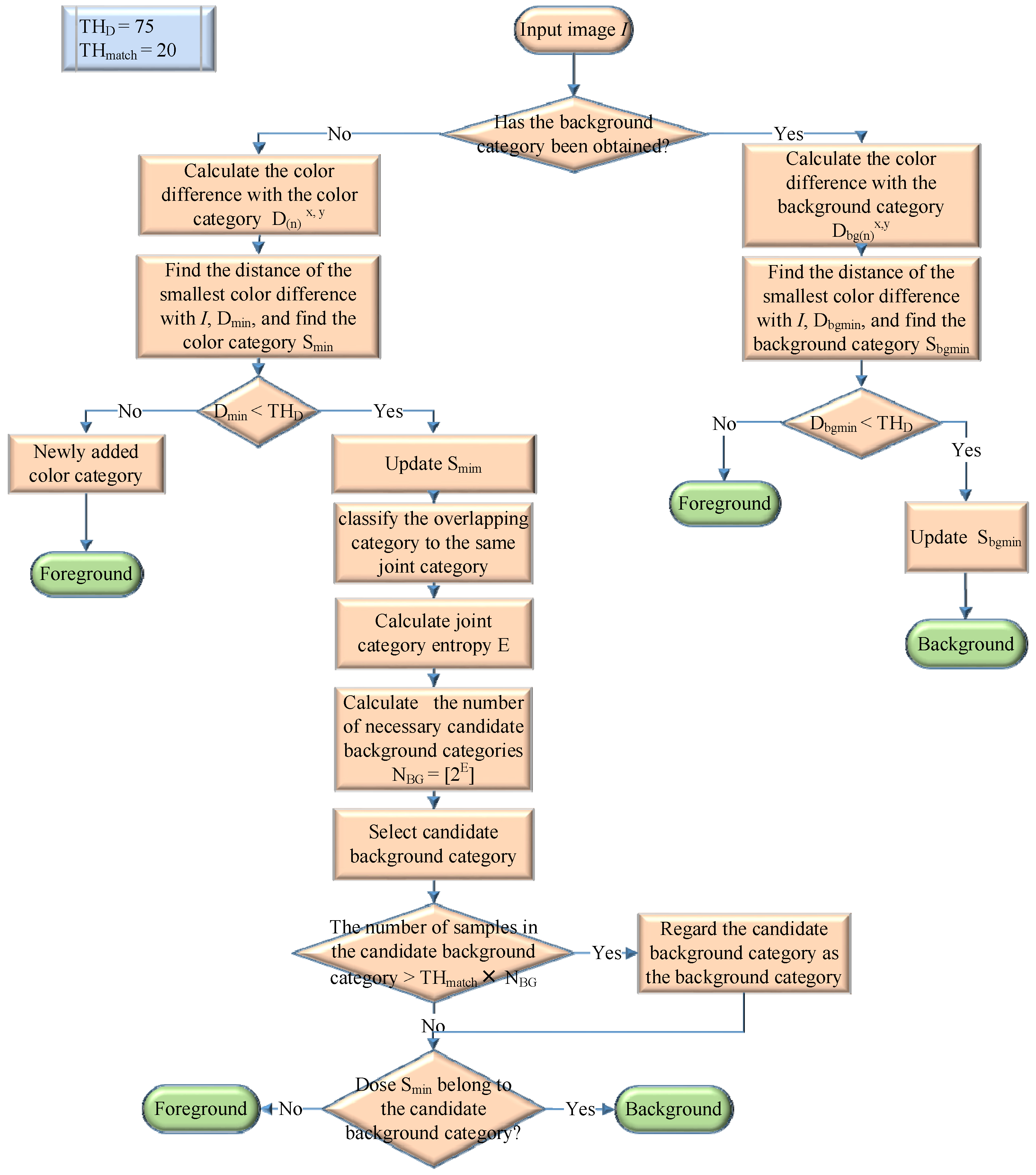Figure 1 is a flowchart of the proposed method, with the implementation steps elaborated as follows.

We first obtained the input image I by a camera and defined $I_R^{x,y}$, $I_G^{x,y}$, and $I_B^{x,y}$ as the red, green, and blue color values, respectively, of $I$ at the (x,y) coordinate. In the beginning, when the background category was not yet acquired at position (x,y), we used a color classifier to create the color category S as shown in Equation (1), where $C_{\left(n\right)}^{x,y}$ represents the total number of samples in the nth color category located at the (x,y) coordinate, while $R_{\left(n\right)}^{x,y}$, $G_{\left(n\right)}^{x,y}$, and $B_{\left(n\right)}^{x,y}$ represent the red, green, and blue color values in the nth color category at the (x,y) coordinate, respectively. $N^{x,y}$ is the total number of color categories at the (x,y) coordinate.

$$\{\begin{array}{c}{S}^{x,y}=\left\{S_{\left(n\right)}^{x,y}|n=1,2,\dots ,N^{x,y}\right\}\\ S_{\left(n\right)}^{x,y}=\left\{C_{\left(n\right)}^{x,y},R_{\left(n\right)}^{x,y},G_{\left(n\right)}^{x,y},B_{\left(n\right)}^{x,y}\right\}.\end{array}$$

(1)

When starting to process the first input image, we created the initial color category $S_{\left(1\right)}^{x,y}$ at its corresponding position (x,y), namely $C_{\left(1\right)}^{x,y}=1$, $R_{\left(1\right)}^{x,y}$ = $I_R^{x,y}$, $G_{\left(1\right)}^{x,y}$ = $I_G^{x,y}$, and $B_{\left(1\right)}^{x,y}$ = $I_B^{x,y}$. The color information of each pixel in the third and later images was clustered with a color distance classifier as explained below. First, we used Equation (2) to calculate the Euclidean distance $D_{\left(n\right)}^{x,y}$ between the input pixel and all the color categories at its position, where $\Delta R_{\left(n\right)}^{x,y}$, $\Delta G_{\left(n\right)}^{x,y}$, and $\Delta B_{\left(n\right)}^{x,y}$ represent the color difference between the input pixel and the red, green, and blue color values in the nth color category at the location, respectively.

$$D_{\left(n\right)}^{x,y}=\sqrt{\Delta R_{\left(n\right)}^{x,y}{}^2+\Delta G_{\left(n\right)}^{x,y}{}^2+\Delta B_{\left(n\right)}^{x,y}{}^2},$$

(2)

$$\Delta R_{\left(n\right)}^{x,y}=I_R^{x,y}-R_{\left(n\right)}^{x,y},$$

$$\Delta G_{\left(n\right)}^{x,y}=I_G^{x,y}-G_{\left(n\right)}^{x,y},$$

$$\Delta B_{\left(n\right)}^{x,y}=I_B^{x,y}-B_{\left(n\right)}^{x,y}.$$

Second, we determined the color category $S_{\min }^{x,y}$, which has the smallest color difference among input pixels, and recorded its index $N_{\min }^{x,y}$ and distance $D_{\min }^{x,y}$ as shown by Equations (3)–(5). Third, we used a color classifier to define a color difference threshold value ${\mathrm{TH}}_D$ to be compared with $D_{min}^{x,y}$. If $D_{min}^{x,y}>{\mathrm{TH}}_D$, it means that the input pixel does not belong to any existing color category. We added a new color category with the color information of the pixel and determined its position as a foreground. If $D_{min}^{x,y}\le {\mathrm{TH}}_D$, it means that the input pixel belongs to the $N_{\min }^{x,y}$-th color category and we increased the number of samples in this color category according to $C_{\left(N_{\min }^{x,y}\right)}^{x,y}=C_{\left(N_{\min }^{x,y}\right)}^{x,y}+1$. In the meantime, we used Equation (6) to update the color information of this category in a progressive manner. Compared with the method of directly calculating the average value of all samples in the color categories, our method improves the computation speed and saves storage space.

$$D_{\min }^{x,y}=\underset{\forall n}{\min }{D}_{\left(n\right)}^{x,y},$$

(3)

$$N_{\min }^{x,y}=\arg \underset{\forall n}{\min }{D}_{\left(n\right)}^{x,y},$$

(4)

$$S_{\min }^{x,y}=\left\{S_{\left(n^{\prime }\right)}^{x,y}\right|n^{\prime }=N_{\min }^{x,y}\},$$

(5)

$$If{\mathrm{R}}_{\left(n^{\prime }\right)}^{x,y}<{\mathrm{I}}_R^{x,y}then{\mathrm{R}}_{\left(n^{\prime }\right)}^{x,y}={\mathrm{R}}_{\left(n^{\prime }\right)}^{x,y}+1,$$

(6)

$$else{R}_{\left(n^{\prime }\right)}^{x,y}=R_{\left(n^{\prime }\right)}^{x,y}-1,$$

$$If{G}_{\left(n^{\prime }\right)}^{x,y}<I_G^{x,y}then{G}_{\left(n^{\prime }\right)}^{x,y}=G_{\left(n^{\prime }\right)}^{x,y}+1where{n}^{\prime }=N_{\min }^{x,y},$$

$$else{G}_{\left(n^{\prime }\right)}^{x,y}=G_{\left(n^{\prime }\right)}^{x,y}-1,$$

$$If{B}_{\left(n^{\prime }\right)}^{x,y}<I_B^{x,y}then{B}_{\left(n^{\prime }\right)}^{x,y}=B_{\left(n^{\prime }\right)}^{x,y}+1,$$

$$else{B}_{\left(n^{\prime }\right)}^{x,y}=B_{\left(n^{\prime }\right)}^{x,y}-1.$$

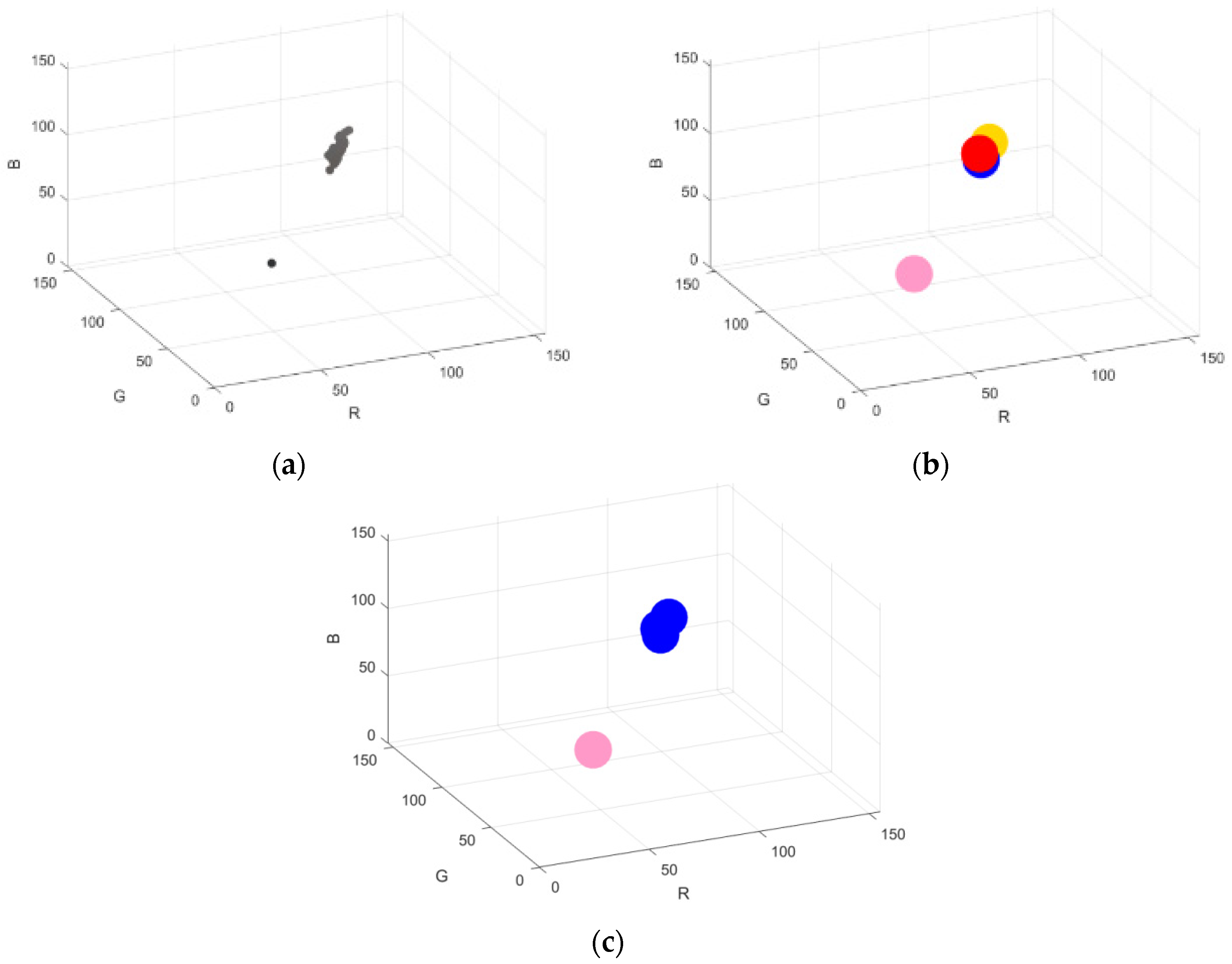
Given that the background color does not change in a short time, when $D_{min}^{x,y}\le {\mathrm{TH}}_D$, this position $\left(x,y\right)$ is represented as a color class $S_{\min }^{x,y}$ similar to the input pixel $I^{x,y}$. If the probability of the occurrence of $S_{\min }^{x,y}$ is higher, it is more likely that input pixel $I^{x,y}$ is the background. However, the background will be subject to varying degrees of disturbance depending on image quality in a real environment, as shown in Figure 2a. If the degree of color disturbance is greater than the color difference threshold ${\mathrm{TH}}_D$, then the background colors cannot be classified in the same category. As shown by the color classification results in Figure 2b, the color distribution at the upper right cannot fall into a single-color category. In addition, the color category established by the color distance classifier has a spherical color-distribution range with a radius of ${\mathrm{TH}}_D$, while the distribution of background colors is irregular depending on the camera quality, as shown in Figure 2a. The increase of ${\mathrm{TH}}_D$ alone will cause large color errors in the background category. Therefore, a joint category approach is proposed to adapt to the irregular color distribution of a real background. The method for color-category information updates used in this study, as shown by Equation (6), will cause the position of the established color category in the RGB color space to change with the change of the input image, thereby causing some color categories to overlap in the color distribution ranges. In this study, the color categories with overlapping color-distribution ranges were considered to belong to the same joint category as shown in Equation (7), where $U_{\left(m\right)}^{x,y}$ represents the mth joint category. Since the color distribution range of a joint category will be arbitrarily extended depending on the color category, it represents the irregular color distribution of a real background, as shown in Figure 2c.

$$U_{\left(m\right)}^{x,y}=\left\{\forall S_{\left(n\right)}^{x,y}|S_{\left(n\right)}^{x,y}\cap S_{\left(m\right)}^{x,y}!=\varnothing , m\le n\le N^{x,y}\right\}.$$

(7)

Background colors usually do not undergo dramatic changes over a short time; therefore, the joint category with a higher occurrence probability can better represent the distribution of background colors. This study calculated the occurrence probability $P_{\left(m\right)}^{x,y}$ of each joint category according to Equation (8), where $C_{\left(n\right)}^{x,y,m}$ represents the count of the nth color category in the mth joint category, the running variable n of ∑ represents all indices of color categories belonging to the mth joint category, and T represents the number of input images. After obtaining the appearance probability of each joint category, the joint category with the highest occurrence probability is the background. In order to solve the problem in the real environment, the background colors at the same position do not necessarily consist of only one color; sometimes, there are more than two background colors such as the color of a shaking tree or the color of a flowing flag. Hence, the concept of joint category entropy was proposed and the change in joint category entropy was used to dynamically determine the required number of candidate background categories as elaborated below. First, joint category entropy was calculated according to Equation (9). Second, joint category entropy (E), was used to automatically determine the number of necessary candidate background categories, as shown in Equation (10), where $N_{BG}^{x,y}$ represents the number of necessary candidate background categories at the (x,y) coordinate. Third, the created joint categories were sorted in the order of decreasing occurrence probabilities, of which the first $N_{BG}^{x,y}$ joint categories were selected as the candidate background categories $S_{BG}^{x,y}$, as shown in Equation (11). Conversely, when no background category has been obtained, if an input pixel is classified as a candidate background category $S_{BG}^{x,y}$, then the input pixel is treated as a background. Conversely, if an input pixel does not belong to a candidate background category, then the input pixel is considered as the foreground. 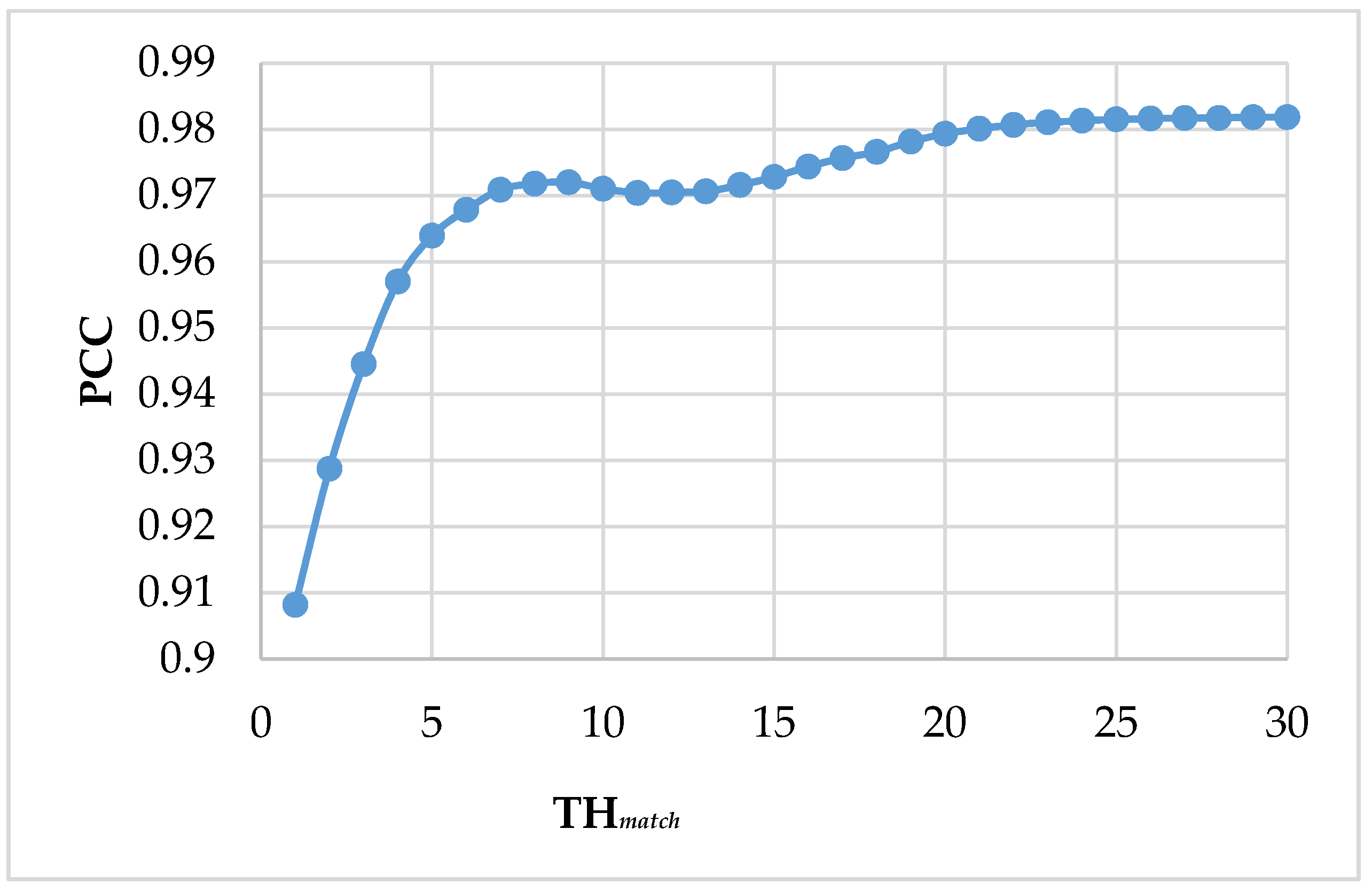When the number of samples belonging to a candidate background category is greater than $T{H}_{match}\times N_{BG}^{x,y}$, the candidate background category is treated as a background category, to which the subsequent input images will be directly compared, with no more selection of candidate background categories. $T{H}_{match}$ indicates the required number of samples allowing the joint categories to be regarded as the background. The $T{H}_{match}$ used in this paper is 20 (see Results and Discussion in Section 4.3: Determination of parameters).

$$P_{\left(m\right)}^{x,y}=\frac{\sum C_{\left(n\right)}^{x,y,m}}{T}, where n=1,2,\dots ,N^{x,y},$$

(8)

$$E^{x,y}=-\sum P_{\left(m\right)}^{x,y}{\log }_2{P}_{\left(m\right)}^{x,y}, where P_{\left(m\right)}^{x,y}>0,$$

(9)

$$N_{BG}^{x,y}=\left[2^{E^{x,y}}\right],$$

(10)

$$S_{BG}^{x,y}=\left\{U_{\left(m\right)}^{x,y}|m=1,\dots ,N_{BG}^{x,y}\right\}.$$

(11)

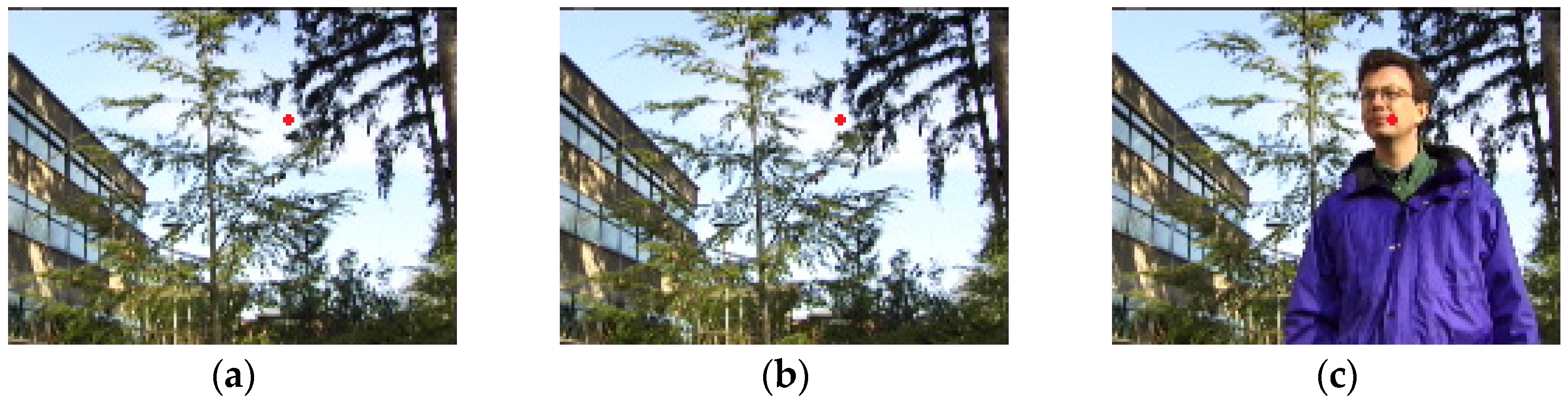
Figure 3 shows the color change of a video series at the sampling position (100, 40). As shown in Figure 3d, the color distribution at this position is quite concentrated in the first 100 images. This position was a stable background point, but in the 250th image, the color distribution at the position changed because of a pedestrian passing through the sampling position, as shown in Figure 3e.

Table 1. Color classification results of the first 250 input images at the coordinate (100, 40).

Image Interval	Joint-Category Number m	${\mathit{S}}^{\mathit{x},\mathit{y}}$	${\mathit{C}}_{\left(\mathit{n}\right)}^{\mathit{x},\mathit{y}}$	${\mathit{P}}_{\left(\mathit{m}\right)}^{\mathit{x},\mathit{y}}$	${\mathit{E}}^{\mathit{x},\mathit{y}}$	${\mathit{N}}_{\mathit{B}\mathit{G}}^{\mathit{x},\mathit{y}}$
1~100	1	(245, 252, 255)	100	100%	0	1
1~250	1	(250, 252, 255)	245	98%	0.16886	1
	2	(250, 191, 133)	3	1.2%
	3	(143, 86, 32)	1	0.4%
	4	(182, 111, 81)	1	0.4%

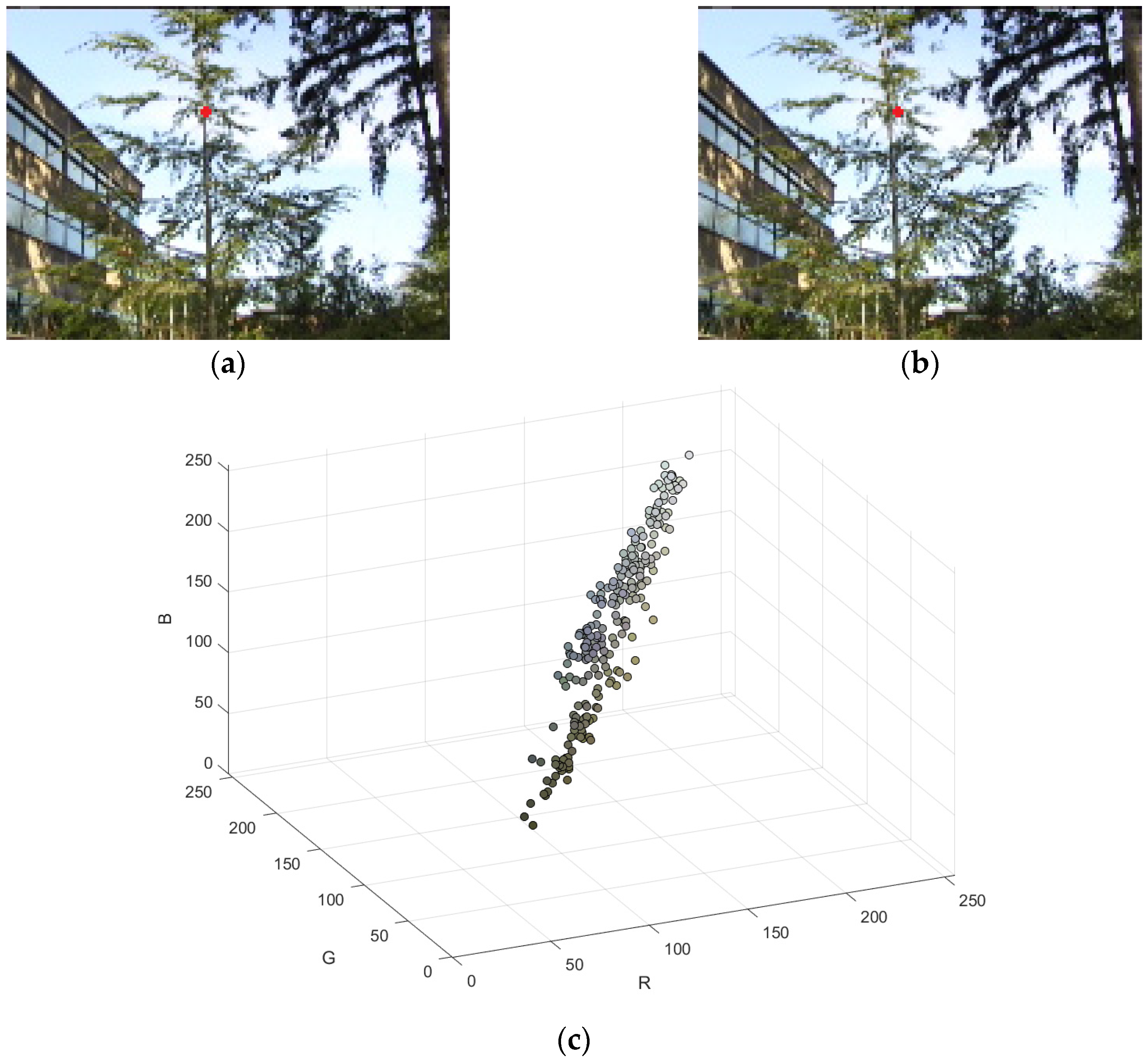
shows the results of joint category clustering at the sampling position. Figure 4 shows the color change of an image sequence at the sampling location (72, 38). Owing to the presence of a shaking tree at the sampling location, the color distribution of the sampling location was dispersed, as shown in Figure 4c.

Table 2. Color classification results of the first to 250th input images at the coordinate (72, 38).

Image Interval	Joint-Category Number m	${\mathit{S}}^{\mathit{x},\mathit{y}}$	${\mathit{C}}_{\left(\mathit{n}\right)}^{\mathit{x},\mathit{y}}$	${\mathit{P}}_{\left(\mathit{m}\right)}^{\mathit{x},\mathit{y}}$	${\mathit{E}}^{\mathit{x},\mathit{y}}$	${\mathit{N}}_{\mathit{B}\mathit{G}}^{\mathit{x},\mathit{y}}$
1~250	1	(164, 170, 169)	40	48%	1.51662	3
		(195, 204, 199)	8
	2	(128, 133, 140)	28	28%
	3	(101, 101, 75)	24	24%

shows the results of joint category clustering at the sampling location. Table 1 and Table 2 show that the proposed joint category entropy E can reflect the stability of pixel color changes and the number of representative categories. A lower E indicates a more concentrated color distribution of the points, and thereby a smaller number of candidate background categories. A higher E indicates a more dispersed color distribution of the points, and thereby a larger number of candidate background categories.

The initial-background capture method proposed in this study used a color classifier to create pixel-based color categories for input images. Based on the joint category concept, it could adapt to the scenario in which background pixels were subjected to color disturbance because of poor image quality or a low frame rate. Moreover, based on the color clustering of each pixel in the images, this study proposed the concept of joint category entropy to dynamically determine the number of candidate background categories required for each pixel. This made it possible to establish a suitable number of background categories for foreground detection, even in harsh background environments such as dynamic backgrounds or a background with camera shake.

4. Results and Discussion

In this section, we discuss the selection of the best parameters for our proposed algorithm, which was also compared with several algorithms established in recent years. This discussion is divided into four parts: introduction of datasets, selection of performance metrics, determination of parameters, and performance testing of other algorithms.

4.1. Introduction of Dataset

Benchmark datasets are critical to the qualitative and quantitative analysis of algorithms. We selected four image segments from two benchmark datasets with ground-truths, Carnegie Mellon [26] and Change Detection.Net (CDW) [27,28], to verify algorithm performance. The features of the selected sequences are described below.

• Carnegie Mellon: This dataset has only one image sequence containing 500 original images with artificially labeled ground-truths. There was a slight camera shake in the image sequence.
• Change Detection.Net: The images of this dataset were classified into 11 attributes—all containing artificially labeled ground-truths. Some of the images only provided ground-truths in the region of interest rather than in the entire region covered by the images. We selected five image sequences from the CDW dataset for testing, each of which was challenging to some extent, as elaborated below.

  (i)

  Skating: This sequence was taken in snowy weather. There were skaters and falling snowflakes in the sequence.

  (ii)

  Highway: There were many moving vehicles and light changes caused by floating clouds in this sequence; there were also shaking trees on the left side of the sequence.

  (iii)

  tramCrossroad_1fps: This sequence was taken at a busy intersection. There were many moving vehicles in the image, as well as flashing billboards. There was only one frames per second (fps) for this sequence.

  (iv)

  Badminton: This sequence was captured at a badminton court. There were some players in the sequence, and there was a violent camera shake.

  (v)

  Sofa: This sequence was captured in a lobby; there were some guests in the sequence.

4.2. Selection of Performance Metrics

Figure 5a shows an input image from a sequence. The detection results of the background subtraction method can be binarized into a cut image, whose background and foreground may be represented by black and white colors, respectively, as shown in Figure 5b. It is possible to evaluate the performance of the background subtraction method by comparing the cut image to the ground-truth cut images. According to the comparison results, the performance can be divided into four types: true positives (TP), meaning the correct detection of foreground pixels; false positives (FP), meaning the incorrect classification of background pixels as foreground pixels; true negatives (TN), meaning the correct classification of background pixels; and false negatives (FN), meaning the incorrect classification of foreground pixels as background pixels.

The greatest difficulty in assessing the performance of background subtraction methods is the lack of standardized assessment criteria, which has prompted scholars to propose evaluation criteria that are only applicable to their algorithms. Therefore, according to [29], we proposed that the percentage of correct classification (PCC) is the most widely used metric for performance evaluation of a binary classifier. This metric contains four values, as shown in Equation (12). This metric was adopted in this study for the performance testing of the background subtraction method. It should be noted that a higher PCC value indicates a more accurate detection result. In order to more objectively evaluate the performance of the algorithm, we further adopted seven metrics such as Equations (13)–(19) [27]. Finally, we used the average ranking $R_i$ to combine the above eight metrics as performance evaluation criteria for different algorithms. The average ranking $R_i$ for method i across all overall average metrics is given by Equation (20), where $m^{\prime }$ is an overall-average metric such as the one in Equation (12) and $ran{k}_i\left(m^{\prime }\right)$ denotes the rank of method i according to the overall-average metric $m^{\prime }$.

$$\mathrm{PCC}=\frac{\mathrm{TP}+\mathrm{TN}}{\mathrm{TP}+\mathrm{TN}+\mathrm{FP}+\mathrm{FN}},$$

(12)

$$\mathrm{Recall}\left(\mathrm{Re}\right)=\frac{\mathrm{TP}}{\mathrm{TP}+\mathrm{FN}},$$

(13)

$$\mathrm{Specificity}\left(\mathrm{Sp}\right)=\frac{\mathrm{TN}}{\mathrm{TN}+\mathrm{FP}},$$

(14)

$$\mathrm{False}\mathrm{Positive}\mathrm{Rate}\left(\mathrm{FPR}\right)=\frac{\mathrm{FP}}{\mathrm{FP}+\mathrm{TN}},$$

(15)

$$\mathrm{False}\mathrm{Negative}\mathrm{Rate}\left(\mathrm{FNR}\right)=\frac{\mathrm{FN}}{\mathrm{FN}+\mathrm{TP}},$$

(16)

$$\mathrm{Percentage}\mathrm{of}\mathrm{Wrong}\mathrm{Classifications}\left(\mathrm{PWC}\right)=100\frac{\mathrm{FN}+\mathrm{FP}}{\mathrm{TP}+\mathrm{TN}+\mathrm{FP}+\mathrm{FN}},$$

(17)

$$\mathrm{Precision}\left(\mathrm{Pr}\right)=\frac{\mathrm{TP}}{\mathrm{TP}+\mathrm{FP}},$$

(18)

$$\mathrm{F}-\mathrm{measure}=2\frac{\mathrm{FN}}{\mathrm{FN}+\mathrm{TP}},$$

(19)

$$R_i={\displaystyle \sum }_{m^{\prime }}ran{k}_i\left(m^{\prime }\right).$$

(20)

4.3. Determination of Parameters

As discussed before, our proposed algorithm has the following parameters:

• ${\mathrm{TH}}_D$: The spherical radius used for the comparison of a newly entered pixel and the color categories.
• ${\mathrm{TH}}_{match}$: The required number of samples allowing the joint category to be regarded as the background.

${\mathrm{TH}}_D$ represents a perceived color difference. In all our tests, ${\mathrm{TH}}_D$= 75 generated the best detection results. In order to determine the optimal ${\mathrm{TH}}_{match}$, we monitored the change in PCC at different ${\mathrm{TH}}_{match}$ values in images detected with the EBBE method. As shown in Figure 6, ${\mathrm{TH}}_{match}\ge 20$ generated satisfying PCC results, while the computational cost of the algorithm increased with the increase in ${\mathrm{TH}}_{match}$. Therefore, we decided that the optimal setting is ${\mathrm{TH}}_{match}=20$.

4.4. Performance Comparison with Other Algorithms

In this study, we compared our proposed algorithm to six popular background subtraction methods: (i) background modeling and subtraction by codebook construction (codebook, [17]); (ii) adaptive background mixture models for real-time tracking (GMM, [13]); (iii) background and foreground modeling using nonparametric kernel density estimation for visual surveillance (KDE, [15]); (iv) an effective object segmentation system using a probability-based background extraction algorithm (PBBE, [19]); (v) a self-organizing approach to background subtraction for visual surveillance applications (SOBS, [20]); and (vi) ViBe, a universal background subtraction algorithm for video sequences (ViBe, [21]).

In order to test the detection capability of the algorithms in a complex background environment, we chose to start the initial-background extraction when there were moving objects in the image sequence, using the start image number of selected image sequences shown in

Table 3. Selected images and the start time of detection.

Database	Image Names	Start Image Number
Carnegie Mellon	Carnegie Mellon	#300
Change Detection.Net	Baseline/highway	#860
Change Detection.Net	badWeather/skating	#800
Change Detection.Net	lowFramerate/tramCrossroad_1fps	#522
Change Detection.Net	cameraJitter/badminton	#800
Change Detection.Net	intermittentObjectMotion/sofa	#2370

. Figure 7, Figure 8, Figure 9 and Figure 10 show the foreground/background detection results of the seven algorithms under different circumstances, with (a) representing the nth input image (initial image), (b) representing the n + 99th input image, and (c)–(j) representing the ground-truth of the n + 99th input image, as well as the foreground/background detection results of the seven methods, with the white pixels and black pixels representing the foreground and background, respectively.

Figure 7 shows the foreground/background detection results obtained by the seven algorithms for one image in the Carnegie Mellon sequence. Owing to the slight camera shake in this image sequence, the background pixels (such as those on the background profile) with relatively large changes of the surrounding colors in the images were likely to produce more than two kinds of color changes. A comparison of Figure 7d–j indicated that the GMM, KDE, PBBE, and SOBS algorithms were affected by camera shake, and thereby mistook many background contours for the foreground, whereas EBBE, codebook, and ViBe had good adaptability to camera shake. However, some of the backgrounds in the initial images were temporarily obscured by a pedestrian, causing codebook, KDE, SOBS, and ViBe to generate many false foregrounds (ghosting) at the position where the pedestrian first appeared on the right side of the images. Only EBBE showed good detection results in scenarios with camera shake and initial-background masking.

Figure 8 shows the foreground/background detection results obtained by the seven algorithms for one image in the highway sequence. Given the effect of a floating cloud on the image lighting, there were slight changes in image brightness. Moreover, there were shaking trees, as well as a large number of moving vehicles, on the left side of the image. A comparison of Figure 8d–j indicated that the codebook, KDE, PBBE, and SOBS algorithms could not adapt to dynamic background environments such as those with a light change and shaking trees, and thereby generated many incorrect foregrounds. With the exception of EBBE, the other algorithms could not overcome the background masking issue due to a large number of moving objects in the background extraction process and generated many erroneous foreground-detection results.

Figure 9 shows the foreground/background detection results obtained by the seven algorithms for one image in the skating sequence. Since this image sequence was taken in snowy weather, there were a lot of snowflakes and skaters in the image. A comparison of Figure 9d–j indicated that the codebook, GMM, PBBE, and SOBS algorithms were not able to adapt to snowy weather conditions—a kind of dynamic background—and incorrectly detected many foregrounds. Given the interfering effect of skaters in the initial background, SOBS and ViBe generated obviously incorrect foregrounds. Despite the tiny fragments in the foregrounds detected by EBBE because of the similarity of the skaters’ clothing to the background, this method was still the closest to the ground-truth approach among the seven methods.

Figure 10 shows the foreground/background detection results obtained by the seven algorithms for one image in the tramCrossroad_1fps sequence, whose dataset only contained ground-truths in the region of interest (non-gray parts) shown in Figure 10c. Since this image sequence was taken at a busy intersection, there were a lot of moving vehicles in the image. The low frame rate also subjected the background to severe color disturbance. A comparison of Figure 10d–j indicated that codebook, KDE, PBBE, and SOBS could not adapt to the background disturbance because of the low frame rate, and thereby incorrectly detected many foregrounds. Moreover, affected by the buses in the initial image, SOBS and ViBe also generated significant ghosting, while both EBBE and GMM had good detection results for this image.

Figure 11 shows the foreground/background detection results obtained by the seven algorithms for one image in the badminton sequence. Since this sequence was taken at a badminton court, there were some players in the image. Owing to the intense camera shake in this image sequence, the background pixels with relatively large changes of the surrounding colors in the images were likely to produce more than two kinds of color changes. A comparison of Figure 11d–j indicated that the codebook, GMM, KDE, PBBE, and SOBS algorithms were affected by intense camera shake, and thereby mistook many background contours for the foreground, whereas EBBE and ViBe had good adaptability to intense camera shake.

Figure 12 shows the foreground/background detection results obtained by the seven algorithms for one image in the sofa sequence. Since this sequence was captured in a lobby, there were some guests in the image. A comparison of Figure 12d–j indicated that codebook, GMM, KDE, PBBE, SOBS, and ViBe were affected by the slow-moving objects in the sequence and generated significant ghosting. Despite the tiny fragments in the foregrounds detected by EBBE because of the similarity of the guests’ clothing to the background, this method was still the closest to the ground-truth approach among the seven methods.

Figure 13 shows the comparison of the PCC values of the seven algorithms. Our EBBE method has the highest PCC value for all tested images compared with other methods, suggesting that EBBE has a good detection accuracy.

Table 4. Overall results across all test sequences.

Method	R	PCC	Re	Sp	FPR	FNR	PWC	Pr	F-Measure
EBBE	1.750	0.968	0.978	0.769	0.231	0.022	3.151	0.989	0.983
codebook	4.750	0.908	0.977	0.336	0.664	0.023	9.209	0.925	0.949
GMM	2.000	0.949	0.980	0.536	0.464	0.020	5.137	0.966	0.972
KDE	2.625	0.915	0.980	0.399	0.601	0.020	8.506	0.930	0.953
PBBE	5.250	0.895	0.979	0.268	0.732	0.021	10.455	0.909	0.942
SOBS	7.000	0.823	0.965	0.132	0.868	0.035	17.711	0.843	0.900
ViBe	4.625	0.911	0.969	0.290	0.710	0.031	8.899	0.936	0.952

shows the eight metrics values of seven algorithms across all test sequence. It should be noted that the higher PCC, Re, Sp, Pr, and F-Measure values indicate more accurate detection results. In addition, the lower FPR, FNR, and PWC values represent more accurate test results. According to the average ranking R, the EBBE is the best performing algorithm among the eight metrics in the seven algorithms.

In typical real-time surveillance systems, the camera captures images at 30 frames per second.

Table 5. Comparison of processing speeds expressed in frames per second.

Sequence	Resolution	EBBE	Codebook	GMM	KDE	PBBE	SOBS	ViBe
Carnegie Mellon	360 × 240	76.3	210.5	94.2	114.9	96.0	87.9	364.1
highway	320 × 240	62.0	145.5	88.3	131.0	82.0	116.4	334.1
skating	540 × 360	49.4	90.7	41.7	84.1	61.8	58.1	169.9
tramCrossroad_1fps	640 × 350	52.9	64.1	35.8	56.4	50.6	46.1	213.0
badminton	720 × 480	34.3	54.2	21.8	41.8	34.8	31.6	119.7
sofa	320 × 240	99.0	242.7	80.6	108.7	110.8	85.9	361.5

shows the processing speeds of the seven algorithms in test sequences. All algorithms were implemented on Visual Studio 2015 (Microsoft Corporation, Redmond, WA, USA). The processor used in our experimental computer was an Intel Core i7-4790 (3.6 GHz) (Intel Corporation, Santa Clara, CA, USA), on which the EBBE algorithm detected objects at a speed higher than 30 frames per second in all test sequences. The proposed algorithm can be applied to real-time surveillance systems.

5. Conclusions

In recent studies on background subtraction, most initial backgrounds were extracted under stable background conditions. Few studies have been conducted on the initial background extraction issue encountered in harsh background conditions such as background masking, dynamic backgrounds, and color disturbance. In this study, an initial background extraction algorithm referred to as EBBE—based on category entropy—was proposed for poor initial-background conditions. This algorithm can adapt to color disturbance due to poor quality cameras or a very low frame rate by establishing joint categories during the initial-background extraction process in order to prevent the background being mistaken for the foreground owing to excessive color disturbance. By using the joint category entropy to dynamically establish representative background categories, the algorithm can overcome the background extraction problem due to camera shake and dynamic background conditions. Compared with established algorithms, the EBBE algorithm reduces the generation of false foregrounds in circumstances where there are large color disturbances due to complex conditions like camera shake, shaking trees, and snowflakes, or due to a very low frame rate. Even in cases of background masking due to moving objects in the initial images, the method was able to find the true background categories through joint category entropy analysis, thus achieving good moving object detection results.

References

1. Lipton, A.J.; Fujiyoshi, H.; Patil, R.S. Moving target classification and tracking from real-time video. In Proceedings of the Fourth IEEE Workshop on Applications of Computer Vision. WACV’98 (Cat. No.98EX201), Princeton, NJ, USA, 19–21 October 1998; IEEE: Princeton, NJ, USA, 1998; Volume 98, pp. 8–14. [Google Scholar]
2. Sindhia, L.; Hariharan, K.; Kumar, D. Efficient Detection Tracking of Multiple Moving Objects in Temporal Domain. In Proceedings of the International Conference on Recent Trends in Information Technology, Chennai, India, 8–9 April 2016. [Google Scholar]
3. Gibson, J.J. The Stimulus Variables for Visual Depth and Distance—The Active Observer. In The Perception of the Visual World; Houghton Mifflin: Boston, MA, USA, 1950; pp. 117–144. ISBN 1114828084. [Google Scholar]
4. Zinbi, Y.; Chahir, Y. Moving object Segmentation; using optical flow with active contour model. In Proceedings of the 2008 3rd International Conference on Information and Communication Technologies: From Theory to Applications, Damascus, Syria, 7–11 April 2008. [Google Scholar]
5. Kim, W.; Jung, C. Illumination-Invariant Background Subtraction : Comparative Review, Models, and Prospects. IEEE Access 2017, 5, 8369–8384. [Google Scholar] [CrossRef]
6. Choudhury, S.K.; Sa, P.K.; Bakshi, S.; Majhi, B. An Evaluation of Background Subtraction for Object Detection Vis-a-Vis Mitigating Challenging Scenarios. IEEE Access 2016, 4, 6133–6150. [Google Scholar] [CrossRef]
7. Bouwmans, T. Recent Advanced Statistical Background Modeling for Foreground Detection—A Systematic Survey. Recent Patents Comput. Sci. 2011, 4, 147–176. [Google Scholar]
8. Vo, G.D.; Park, C. Robust regression for image binarization under heavy noise and nonuniform background. Pattern Recognit. 2018, 81, 224–239. [Google Scholar] [CrossRef]
9. Zhiwei, H.Z.H.; Jilin, L.J.L.; Peihong, L.P.L. New method of background update for video-based vehicle detection. In Proceedings of the 7th International IEEE Conference on Intelligent Transportation Systems (IEEE Cat. No.04TH8749), Washington, WA, USA, 3–6 October 2004; pp. 580–584. [Google Scholar]
10. Cheng, F.-C.; Huang, S.-C.; Ruan, S.-J. Advanced motion detection for intelligent video surveillance systems. In Proceedings of the 2010 ACM Symposium on Applied Computing—SAC ’10, Sierre, Switzerland, 22–26 March 2010; ACM: New York, NY, USA, 2010; pp. 983–984. [Google Scholar]
11. Wren, C.R.; Azarbayejani, A.; Darrell, T.; Pentland, A.P. Pfinder: Real-time tracking of the human body. IEEE Trans. Pattern Anal. Mach. Intell. 1997, 19, 780–785. [Google Scholar] [CrossRef]
12. Friedman, N.; RussellImage, S. Segmentation in Video Sequences: A Probabilistic Approach. In Proceedings of the UAI’97 Thirteenth Conference on Uncertainty in Artificial Intelligence, Providence, RI, USA, 1–3 August 1997; Morgan Kaufmann Publishers Inc.: Burlington, MA, USA, 1997; pp. 175–181. [Google Scholar]
13. Stauffer, C.; Grimson, W.E.L. Adaptive background mixture models for real-time tracking. In Proceedings of the 1999 IEEE Computer Society Conference on Computer Vision and Pattern Recognition Cat No PR00149, Fort Collins, CO, USA, 23–25 June 1999; Volume 2, pp. 246–252. [Google Scholar]
14. Stauffer, C.; Grimson, W. Learning Patterns of Activity Using Real-Time Tracking. IEEE Trans. Pattern Anal. Mach. Intell. 2000, 22, 747–757. [Google Scholar] [CrossRef]
15. Elgammal, A.; Davis, L.S. Background and foreground modeling using nonparametric kernel density estimation for visual surveillance. Proc. IEEE 2002, 90, 1151–1163. [Google Scholar] [CrossRef]
16. Li, Q.-Z.; He, D.-X.; Wang, B. Effective Moving Objects Detection Based on Clustering Background Model for Video Surveillance. In Proceedings of the 2008 Congress on Image and Signal Processing, Sanya, Hainan, China, 27–30 May 2008; pp. 656–660. [Google Scholar]
17. Kim, K.; Chalidabhongse, T.H.; Harwood, D.; Davis, L. Background modeling and subtraction by codebook construction. In Proceedings of the 2004 International Conference on Image Processing, ICIP ’04, Singapore, 24–27 October 2004; Volume 5, pp. 3061–3064. [Google Scholar]
18. Kim, K.; Chalidabhongse, T.H.; Harwood, D.; Davis, L. Real-time foreground-background segmentation using codebook model. Real-Time Imaging 2005, 11, 172–185. [Google Scholar] [CrossRef] [Green Version]
19. Chiu, C.C.; Ku, M.Y.; Liang, L.W. A robust object segmentation system using a probability-based background extraction algorithm. IEEE Trans. Circuits Syst. Video Technol. 2010, 20, 518–528. [Google Scholar] [CrossRef]
20. Maddalena, L.; Petrosino, A. A Self-organizing approach to background subtracion for visual surveillance applications. IEEE Trans. Image Process. 2008, 17, 1168–1177. [Google Scholar] [CrossRef] [PubMed]
21. Barnich, O.; Van Droogenbroeck, M. ViBe: A universal background subtraction algorithm for video sequences. IEEE Trans. Image Process. 2011, 20, 1709–1724. [Google Scholar] [CrossRef] [PubMed]
22. Huynh-The, T.; Banos, O.; Lee, S.; Kang, B.H.; Kim, E.S.; Le-Tien, T. NIC: A Robust Background Extraction Algorithm for Foreground Detection in Dynamic Scenes. IEEE Trans. Circuits Syst. Video Technol. 2017, 27, 1478–1490. [Google Scholar] [CrossRef]
23. Huynh-The, T.; Lee, S.; Hua, C.H. ADM-HIPaR: An efficient background subtraction approach. In Proceedings of the 2017 14th IEEE International Conference on Advanced Video and Signal Based Surveillance, AVSS 2017, Lecce, Italy, 29 August–1 September 2017. [Google Scholar]
24. Han, B.; Davis, L.S. Density-Based Multifeature Background Subtraction with Support Vector Machine. IEEE Trans. Pattern Anal. Mach. Intell. 2012, 34, 1017–1023. [Google Scholar] [PubMed]
25. Junejo, I.N.; Ahmed, N. Foreground extraction for moving RGBD cameras. IET Comput. Vis. 2018, 12, 322–331. [Google Scholar] [CrossRef]
26. Sheikh, Y.; Shah, M. Bayesian modeling of dynamic scenes for object detection. IEEE Trans. Pattern Anal. Mach. Intell. 2005, 27, 1778–1792. [Google Scholar] [CrossRef] [PubMed]
27. Wang, Y.; Jodoin, P.M.; Porikli, F.; Konrad, J.; Benezeth, Y.; Ishwar, P. CDnet 2014: An expanded change detection benchmark dataset. In Proceedings of the IEEE Computer Society Conference on Computer Vision and Pattern Recognition Workshops, Columbus, OH, USA, 23–28 June 2014; pp. 393–400. [Google Scholar]
28. Goyette, N.; Jodoin, P.-M.; Porikli, F.; Konrad, J.; Ishwar, P. Changedetection.net : A New Change Detection Benchmark Dataset. In Proceedings of the IEEE Computer Society Conference on Computer Vision and Pattern Recognition Workshops, Providence, RI, USA, 16–21 June 2012; pp. 1–8. [Google Scholar]
29. Ahmed, S.; El-Sayed, K.; Elhabian, S. Moving Object Detection in Spatial Domain using Background Removal Techniques—State-of-Art. Recent Patents Comput. Sci. 2008, 1, 32–54. [Google Scholar] [CrossRef]
Figure 1. Flowchart of the proposed algorithm.
Applsci 08 00885 g001
Figure 2. The process of joint category clustering. (a) Color distribution of the original data, (b) results of color classification, (c) results of joint category clustering.
Applsci 08 00885 g002
Figure 3. The color change of a video series at the sampling position (100, 40): (a) the first input image, (b) the 100th input image, (c) the 250th input image, with the red dot on the diagram representing the sampling position, (d) color distribution of the first to 100th input images, and (e) color distribution of the first to 250th input images.
Applsci 08 00885 g003aApplsci 08 00885 g003b
Figure 4. The color change of a video series at the sampling position (72, 38): (a) the first input image, (b) the 250th input image, with the red dot on the diagram representing the sampling position, and (c) color distribution of the first to 250th input images.
Applsci 08 00885 g004
Figure 5. (a) Input image, (b) foreground.
Applsci 08 00885 g005
Figure 6. Percentage of correct classification (PCC) for TH m a t c h ranging from 1 to 30.
Applsci 08 00885 g006
Figure 7. Comparison of segmentation results of seven background subtraction methods for one frame taken from the Carnegie Mellon sequence. (a) Frame n (start image), (b) frame n + 99, (c) ground-truth, (d) entropy-based initial background extraction (EBBE) (proposed), (e) codebook, (f) Gaussian mixture model (GMM), (g) kernel density estimation (KDE), (h) probability-based background extraction algorithm (PBBE), (i) self-organizing background subtraction (SOBS), and (j) ViBe.
Applsci 08 00885 g007
Figure 8. Comparison of segmentation results of seven background subtraction methods for one frame taken from the highway sequence. (a) Frame n (start image), (b) frame n + 99, (c) ground-truth, (d) EBBE (proposed), (e) codebook, (f) GMM, (g) KDE, (h) PBBE, (i) SOBS, and (j) ViBe.
Applsci 08 00885 g008
Figure 9. Comparison of segmentation results of seven background subtraction methods for one frame taken from the skating sequence. (a) Frame n (start image), (b) frame n + 99, (c) ground-truth, (d) EBBE (proposed), (e) codebook, (f) GMM, (g) KDE, (h) PBBE, (i) SOBS, and (j) ViBe.
Applsci 08 00885 g009
Figure 10. Comparison of segmentation results of seven background subtraction methods for one frame taken from the tramCrossroad_1fps sequence. (a) Frame n (start image), (b) frame n + 99, (c) ground-truth, (d) EBBE (proposed), (e) codebook, (f) GMM, (g) KDE, (h) PBBE, (i) SOBS, and (j) ViBe.
Applsci 08 00885 g010
Figure 11. Comparison of segmentation results of seven background subtraction methods for one frame taken from the badminton sequence. (a) Frame n (start image), (b) frame n + 99, (c) ground-truth, (d) EBBE (proposed), (e) codebook, (f) GMM, (g) KDE, (h) PBBE, (i) SOBS, and (j) ViBe.
Applsci 08 00885 g011
Figure 12. Comparison of segmentation results of seven background subtraction methods for one frame taken from the sofa sequence. (a) Frame n (start image), (b) frame n + 99, (c) ground-truth, (d) EBBE (proposed), (e) codebook, (f) GMM, (g) KDE, (h) PBBE, (i) SOBS, and (j) ViBe.
Applsci 08 00885 g012
Figure 13. PCCs of seven background subtraction methods. (a) Results for the sequence (Carnegie Mellon). (b) Results for the sequence (highway). (c) Results for the sequence (skating). (d) Results for the sequence (tramCrossroad_1fps). (e) Results for the sequence (badminton). (f) Results for the sequence (sofa).
Applsci 08 00885 g013aApplsci 08 00885 g013b