GNSS Positioning Accuracy Enhancement Based on Robust Statistical MM Estimation Theory for Ground Vehicles in Challenging Environments


Abstract
:Featured Application
Abstract
1. Introduction
2. Review of Robust Statistics
3. Least Squares Estimation Model for GNSS Positioning and Outlier Correction
3.1. Least Squares Position Estimation
3.2. Receiver Autonomous Integrity Monitoring Model for Outlier Detection and Removal
4. MM Estimation Theory for Positioning
- Find an initial estimate, with IRWLS (Appendix B) or subsampling method (Appendix C). In IRWLS (simplest subsampling) procedure, all observations are used in estimation. However, in subsampling procedure, subsamples (subsets) of observations are selected each with size of , number of observations in one subset. For each subsample, a solution is computed using IRWLS. Best candidate solution is selected as and the initial residuals are estimated, for each observation. Then we get a residual vector
- Multiple scale estimate functions are defined, however the following median function is employed to compute the initial scale value [33],
- Compute initial scaled residual vector . Use the weighting function of one method, Huber or Bi-square, shown in Table 1 to compute corresponding weights for each observation.
- Solve the estimated unknown at the i-th iteration (i = 1, 2, 3, …) by using the weighted least-squared method,is the transform matrix composed of , and is the weighting matrix with the weights as diagonal elements.
- Update residuals with the new estimate , calculated in last step. Then compute scaled residual . Note that we still use last-step’s scale factor to get new scaled residual because updated scale factor can only be obtained later.
- Use the objective function to compute transformed scaled residual , and get a transformed scaled residual vector .
- Update scale factor with Equation (20) but with the transformed scaled residual vector . After that go back to step 4 to start a new iteration.
5. GNSS Receiver Positioning System Architecture
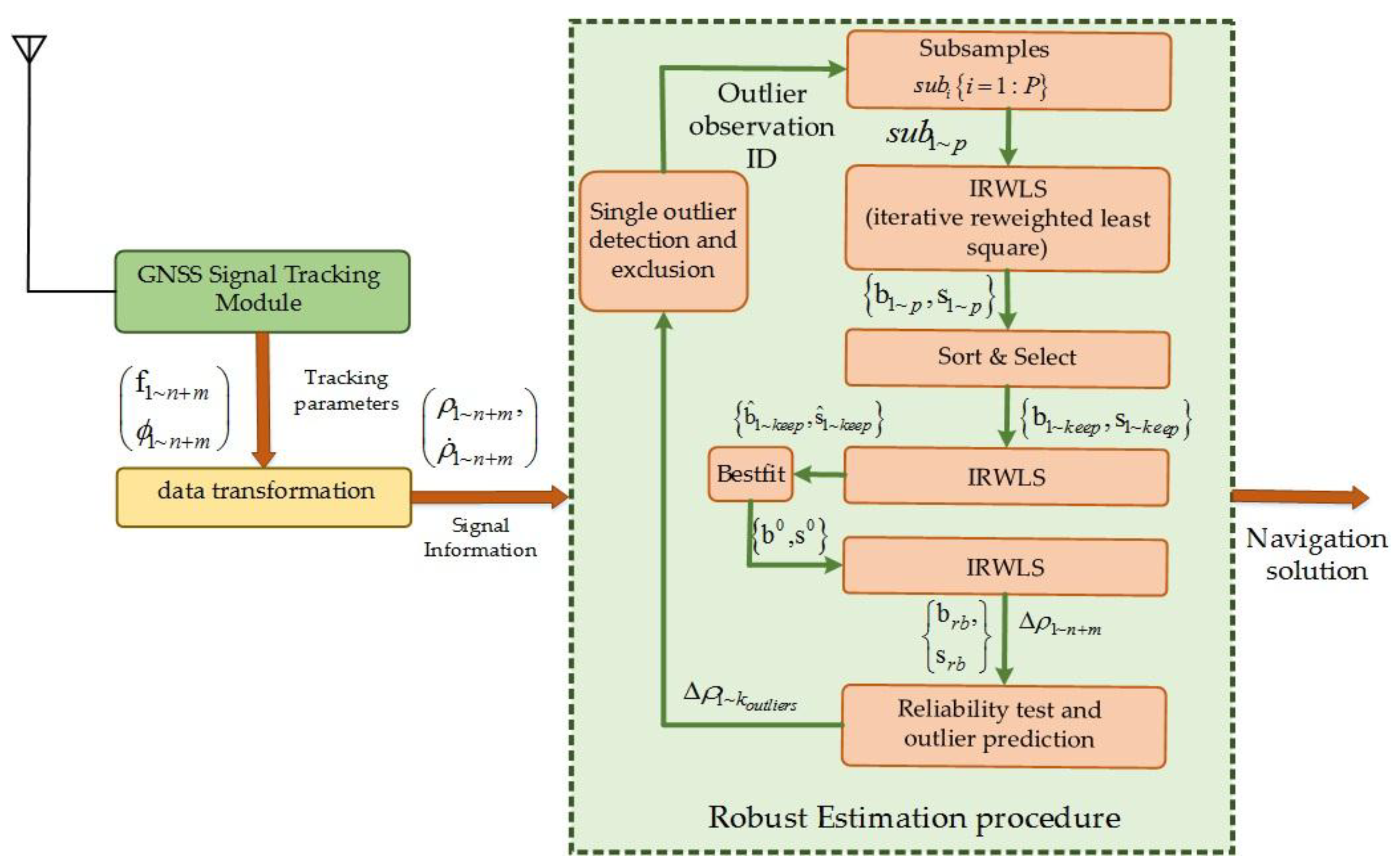
6. Proposed Multiconstellation Positioning Algorithm
6.1. Estimation (Stage 1)
- Select subsamples of size from all observations. The number of the subsamples is,represents the number of observations in one subsample. The value should always meet the criteria of . is the minimal number of observations required for positioning. is selected so that at least one combination contains all observations with high . However, Equation (23) is not directly applicable to a multiconstellation positioning system. For a multiconstellation positioning system, the number of unknowns are , here is the number of constellations used in positioning (clock correction parameters). In order to attain the benefits of the multiconstellation positioning, subsamples must contain at least one observations from each constellation, for example a two constellations based positioning system with five observations independently, maximum four observations can be selected from either constellation to fulfill the minimum requirement as minimum five observations are required for positioning.
- Let is a subsample belonging to where . We compute the initial estimate with the WLSE method,Here , and are the geometry matrix, the observation vector and the weight matrix for the subset . is a diagonal observation weights matrix and initial weights are calculated by using following relation [34].is the predetection integration time and is the code wavelength. is the carrier-to-noise ratio for corresponding satellite signal.
- Compute the residual vector , scale factor and standardized residuals,
- Tukey bi-weight function (Table 1) is adopted to update the weighting matrix .Here is the tuning factor to balance the accuracy and the breakdown robustness and can be selected from the look up table in Appendix A. is selected to maintain 95% efficiency. Then updated weighting matrix will be .
- Use Equation (24) again with updated weight matrix to compute the unknowns, then we get the estimate for the subsample set .
6.2. Estimation (Stage 2)
- Apply steps 1∼5 to all subsets and we get a set of subsample estimates and their corresponding scale factors,Next sort up the scale vector in ascending order as . Take the 5 minimal scale factors from and their corresponding estimates (the number 5 is determined empirically by the authors, it can be changed). Up to now we obtained the most robust 5 initial estimates , their relative scale factors and corresponding subsamples . is the subsample used to compute where . We apply the above steps 1∼5 iteratively to the selected subsets . The iteration stops only when the convergence point is achieved,is set as 0.001. The only difference in this step is the weighting function that we adopt Tukey bi-weight function type 2,Once all the selected 5 subset estimates have got converged, the one with minimal scale factor will be taken as the most robust initial estimate for the final robust estimation.
- Based on the robust initial estimate and its scale factor , we use all observations at this step to get the final robust estimate. The computation procedure is the same as step 1∼5, or equivalently as the IRWLS algorithm in Appendix B. This iteration will not stop until the convergence point, Equation (29) is met, and the final estimate is obtained.
7. Outlier Identification and Exclusion
- A predetection test is performed to predict the possible outlier observations prior to the FDE (fault detection and exclusion) process. A predefined threshold level is used to predict the outlier observations based on the confidence level and on the confidence interval. A confidence interval is the range of values those act as the good estimates and the confidence level is the proportion of the confidence interval that contains the true value of their corresponding parameter. The confidence interval can be calculated from data [35,36]. However, the desired confidence level is defined by the user. Let is the confidence level in predetection test, a threshold can be computed using normal inverse cumulative distribution function (also called quantile function).Here is the probability for corresponding confidence level with mean and standard deviation and is the cumulative distribution function (CDF). The scaled observation residual is computed as,Here and . As soon as follows distribution with degree of freedom, the estimated position is considered as reliable, where is the number of observations used for integrity monitoring and is the number of unknown to be estimated.
- Otherwise, a set of observations is selected as the potential outliers based on the following relation,Let is the set of predicted outlier observations. is corresponding observation number. The FDE on the predicted set of outliers is applied as follows,
8. Discussion
9. Performance Validation and Analysis
9.1. Open Sky Scenario
9.1.1. Emulated Scenario 1
9.1.2. Emulated Scenario 2
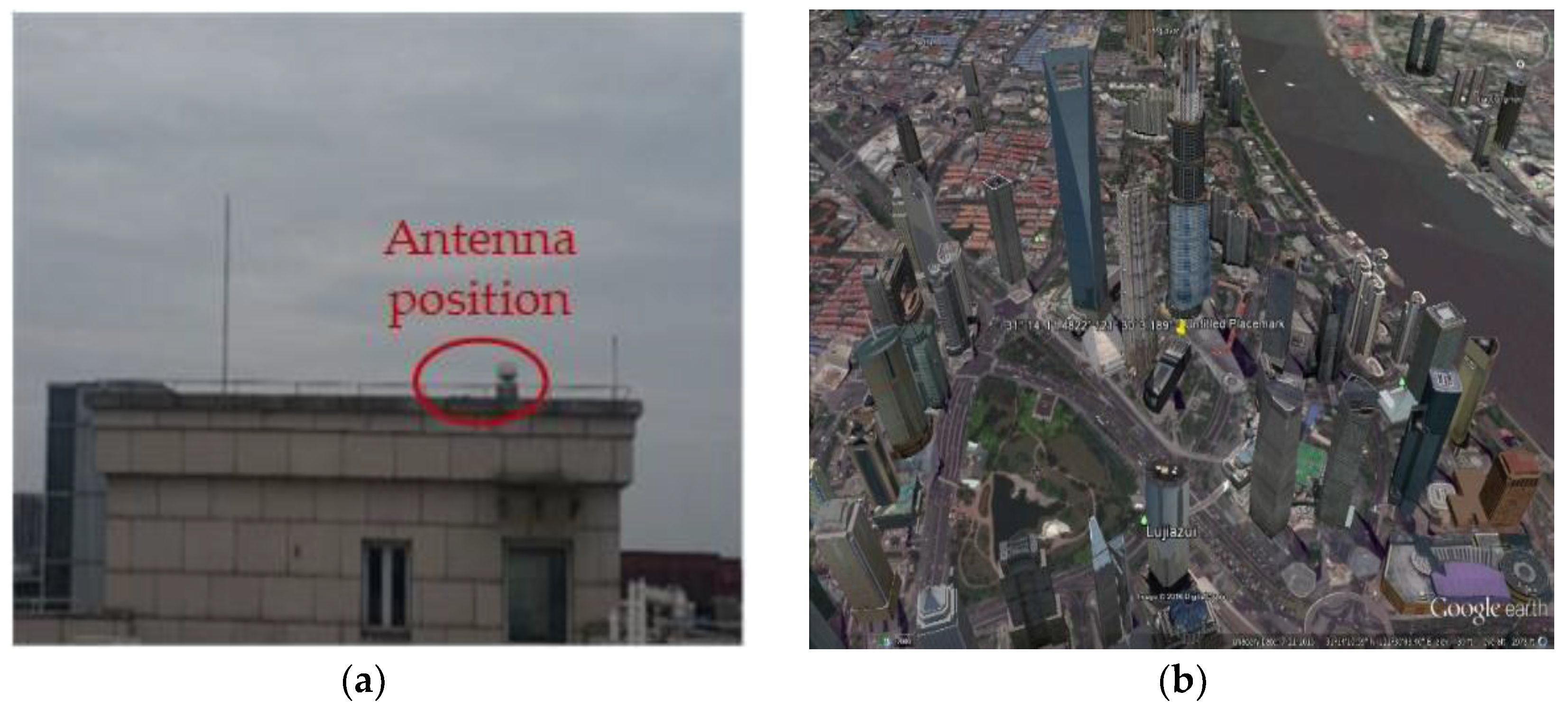
9.2. Multipath Scenario in Urban Canyons
9.3. High Dynamic Moving Scenario
10. Conclusions and Future Perspectives
Author Contributions
Acknowledgments
Conflicts of Interest
Appendix A

| BDP | Efficiency | ||
|---|---|---|---|
| 50% | 28.7% | 1.547 | 0.1995 |
| 45% | 37.0% | 1.756 | 0.2312 |
| 40% | 46.2% | 1.988 | 0.2634 |
| 35% | 56.0% | 2.251 | 0.2957 |
| 30% | 66.1% | 2.560 | 0.3278 |
| 25% | 75.9% | 2.973 | 0.3593 |
| 20% | 84.7% | 3.420 | 0.3899 |
| 15% | 91.7% | 4.096 | 0.4194 |
| 0.10% | 96.6% | 5.182 | 0.4475 |
Appendix B
- Defined convergence constant and calculate initial estimate using weighted least squares using
- Compute initial residual vector using
- Calculate initial standardized residuals;
- Tukey bi-weight function type1 with tuning constant is applied.
- while
- If ; break
- If ; continue
- Calculate using Tukey bi-weight function type 2. is the number of observations.Here
- go to step a.
- end
Appendix C
- Select subsamples of size and number of subsamples.
- Compute initial estimate for each subsample using weighted least squares estimation (WLSE)
References
- Moka, E.; Paul, A. Crossa A Fast Satellite Selection Algorithm for Combined GPS and GLONASS Receivers. J. Navig. 1994, 47, 383–389. [Google Scholar]
- Zhang, M.; Zhang, J. A Fast Satellite Selection Algorithm: Beyond Four Satellites. IEEE J. Sel. Top. Signal Process. 2009, 3, 740–747. [Google Scholar] [CrossRef]
- Zhu, J.J. Calculation of geometric dilution of precision. IEEE Trans. Aerosp. Electron. Syst. 1992, 28, 893–895. [Google Scholar]
- Wei, M.; Wang, J.; Li, J. A new satellite selection algorithm for real-time application. In Proceedings of the International Conference on Systems and Informatics (ICSAI), Yantai, China, 19–20 May 2012; pp. 2567–2570. [Google Scholar]
- Kong, J.; Mao, X.; Li, S. BDS/GPS satellite selection algorithm based on polyhedron volumetric method. In Proceedings of the IEEE/SICE International Symposium on System Integration (SII), Tokyo, Japan, 13–15 December 2014; pp. 340–345. [Google Scholar]
- Zhang, X.Y.; Huang, Z.G.; Li, R. RAIM analysis in the position domain. In Proceedings of the IEEE/ION Position Location and Navigation Symposium (PLANS), Indian Wells, CA, USA, 4–6 May 2010; pp. 53–59. [Google Scholar]
- Hewitson, S.; Lee, H.K.; Wang, J. Localizability Analysis for GPS/Galileo Receiver Autonomus Integrity Monitoring. J. Navig. 2004, 57, 245–259. [Google Scholar] [CrossRef]
- Baarda, W. A Testing Procedure for Use in Geodetic Networks. Netherlands Geodetic Commission; Publications on Geodesy, New Series 2, No. 5; Rijkscommissie voor Geodesie: Delft, The Netherlands, 1968. [Google Scholar]
- Blanch, J.; Ene, A.; Walter, T.; Enge, P. An Optimized Multiple Hypothesis RAIM Algorithm for Vertical Guidance. In Proceedings of the 20th ITM, The Institute of Navigation, Fort Worth, TX, USA, 25–28 September 2007; pp. 2924–2933. [Google Scholar]
- Martineau, A.; Macabiau, C.; Mabilleau, M. GNSS RAIM assumptions for vertically guided approaches. In Proceedings of the 22nd International Technical Meeting of The Satellite Division of the Institute of Navigation, Savannah, GA, USA, 22–25 September 2009; The Institute of Navigation: Savannah, GA, USA, 2009; pp. 2791–2803. [Google Scholar]
- Kaplan, E.D.; Hegarty, C.J. Understanding GPS, Principles and Applications, 2nd ed.; Artech House: Norwood, MA, USA, 2005. [Google Scholar]
- Li, J.; Wu, M. The Improvement of Positioning Accuracy with Weighted Least Square Based on SNR. In Proceedings of the 2009 5th International Conference on Wireless Communications, Networking and Mobile Computing, Beijing, China, 24–26 September 2009; pp. 1–4. [Google Scholar]
- Tabatabaei, A.; Mosavi, M.R.; Khavari, A. Reliable Urban Canyon Navigation Solution in GPS and GLONASS Integrated Receiver Using Improved Fuzzy Weighted Least-Square Method. Wirel. Pers. Commun. 2017, 94, 3181–3196. [Google Scholar] [CrossRef]
- Rahemi, N. Accurate Solution of Navigation Equations in GPS Receivers for Very High Velocities Using Pseudorange Measurements. Adv. Aerosp. Eng. 2014, 2014, 435891. [Google Scholar] [CrossRef]
- Tay, S.; Marais, J. Weighting models for GPS Pseudorange observations for land transportation in urban canyons. In Proceedings of the 6th European Workshop on GNSS Signals and Signal Processing, Munich, Germany, 5–6 December 2013. [Google Scholar]
- Jwo, D.J.; Chang, S.J. Outlier Resistance Estimator for GPS Positioning. In Proceedings of the 2006 IEEE International Conference on Systems, Man and Cybernetics, Taipei, Taiwan, 8–11 October 2006; pp. 657–662. [Google Scholar]
- Rao, K.D.; Swamy, M.N.S.; Plotkin, E.I. GPS navigation with increased immunity to modeling errors. IEEE Trans. Aerosp. Electron. Syst. 2004, 40, 2–11. [Google Scholar]
- Fallahi, K.; Cheng, C.T.; Fattouche, M. Robust Positioning Systems in the Presence of Outliers Under Weak GPS Signal Conditions. IEEE Syst. J. 2012, 6, 401–413. [Google Scholar] [CrossRef]
- Kim, E.; Walter, T.; Powell, J.D. Adaptive carrier smoothing using code and carrier divergence. In Proceedings of the ION NTM, San Diego, CA, USA, 22–24 January 2007; pp. 114–152. [Google Scholar]
- Yoon, D.; Kee, C.; Seo, J.; Park, B. Position Accuracy Improvement by Implementing the DGNSS-CP Algorithm in Smartphones. Sensors 2016, 16, 910. [Google Scholar] [CrossRef] [PubMed]
- Yohai, V.J. High breakdown point and high efficiency robust estimates for regression. Ann. Stat. 1987, 15, 642–656. [Google Scholar] [CrossRef]
- Hampel, F.R. Beyond location parameters: Robust concepts and methods. Bull. Int. Stat. Inst. 1975, 46, 375–391. [Google Scholar]
- Rousseeuw, P.J. Least median of squares regression. J. Am. Stat. Assoc. 1984, 79, 871–880. [Google Scholar] [CrossRef]
- Davies, L. The asymptotics of S-estimators in the linear regression model. Ann. Stat. 1990, 18, 1651–1675. [Google Scholar] [CrossRef]
- Rousseeuw, P.J.; Yohai, V. Robust Regression by Means of S-estimates. Robust and Nonlinear Time Series Analysis; Lecture Notes in Stati; Springer: New York, NY, USA, 1984; Volume 26, pp. 256–272. [Google Scholar]
- Hössjer, O. On the optimality of S-estimators. Stat. Probab. Lett. 1992, 14, 413–419. [Google Scholar] [CrossRef]
- Rousseeuw, P.J.; Leroy, A. Robust Regression and Outlier Detection; Wiley: New York, NY, USA, 1987. [Google Scholar]
- Bryan, C.G. Weighted Least-Squares Orbit Estimation using GPS SPS Navigation Solution Data. Master’s Thesis, San Jose State University, San Jose, CA, USA, 1995. [Google Scholar]
- Delgado, N.B.; Nunes, F. Satellite selection based on WDOP concept and convex geometry. In Proceedings of the 5th ESA Workshop on Satellite Navigation Technologies and European Workshop on GNSS Signals and Signal Processing (NAVITEC), Noordwijk, The Netherlands, 8–10 December 2010; pp. 1–8. [Google Scholar]
- Gervini, D.; Yohai, V.J. A class of robust and fully efficient regression estimators. Ann. Stat. 2002, 30, 583–616. [Google Scholar] [CrossRef]
- Rey, W.J. Introduction to Robust and Quasi-Robust Statistical Methods; Springer: Berlin/Heidelberg, Germany, 1983. [Google Scholar]
- Huber, P.J. Robust Statistics; John Wiley & Sons, Inc.: Hoboken, NJ, USA, 2009. [Google Scholar]
- Draper, N.R.; Smith, K. Applied Regression Analysis, 3rd ed.; Wiley: New York, NY, USA, 1998. [Google Scholar]
- Parkinson, B.; Spilker, J. The Global Positioning System: Theory and Applications, ser. Progress in Astronautics and Aeronautics; American Institute of Aeronautics and Astronautics, Inc., SW: Washington, DC, USA, 1996; Volume 1. [Google Scholar]
- Javanmard, A.; Montanari, A. Confidence Intervals and Hypothesis Testing for High-Dimensional Statistical Models. In Proceedings of the Advances in Neural Information Processing Systems 26 NIPS, Lake Tahoe, CA, USA, 5–10 December 2013; pp. 1187–1195. [Google Scholar]
- Cetin, M.; Aktas, S. Confidence Intervals Based on Robust Estimators. J. Mod. Appl. Stat. Methods 2008, 7, 21. [Google Scholar] [CrossRef]
- Brunner, F.; Hartinger, H.; Troyer, L. GPS signal diffraction modelling: The stochastic SIGMA-D model. J. Geodesy 1999, 73, 259. [Google Scholar] [CrossRef]


| Name | Objective Function | Weight Function |
|---|---|---|
| LSE | ||
| Huber | ||
| Bi-square |
| BeiDou Discriminator Output (Integration Time) | GEO | 2 ms |
|---|---|---|
| MEO | 20 ms | |
| GPS Discriminator Output (Integration Time) | MEO | 20 ms |
| DLL bandwidth | 1 Hz | |
| PLL bandwidth | 10 Hz | |
| Position update interval | 1 s | |
| CN0 update interval | 1 s | |
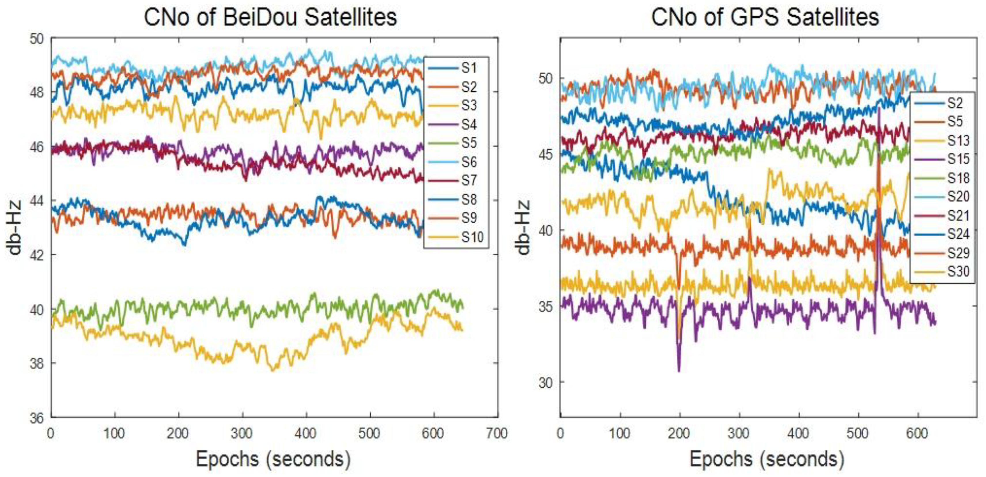
| GNSS | Signal Type | Intermediate Frequency | No. of Satellites | Satellite IDs |
|---|---|---|---|---|
| BeiDou | B1I | −6.902 (MHz) | 10 | 1, 2, 3, 4, 5, 6, 7, 8, 9, 10 |
| GPS | L1-CA | 7.42 (MHz) | 10 | 2, 5, 13, 15, 18, 20, 21, 24, 29, 30 |
| Time (s) | Outliers | Bias (m) | PRN with Bias | |
|---|---|---|---|---|
| BeiDou | GPS | |||
| 1–100 | 0 | 0 | 0 | 0 |
| 101–200 | 1 | 500 | 3 | 0 |
| 201–300 | 2 | [500, 900] | 4, 9 | 0 |
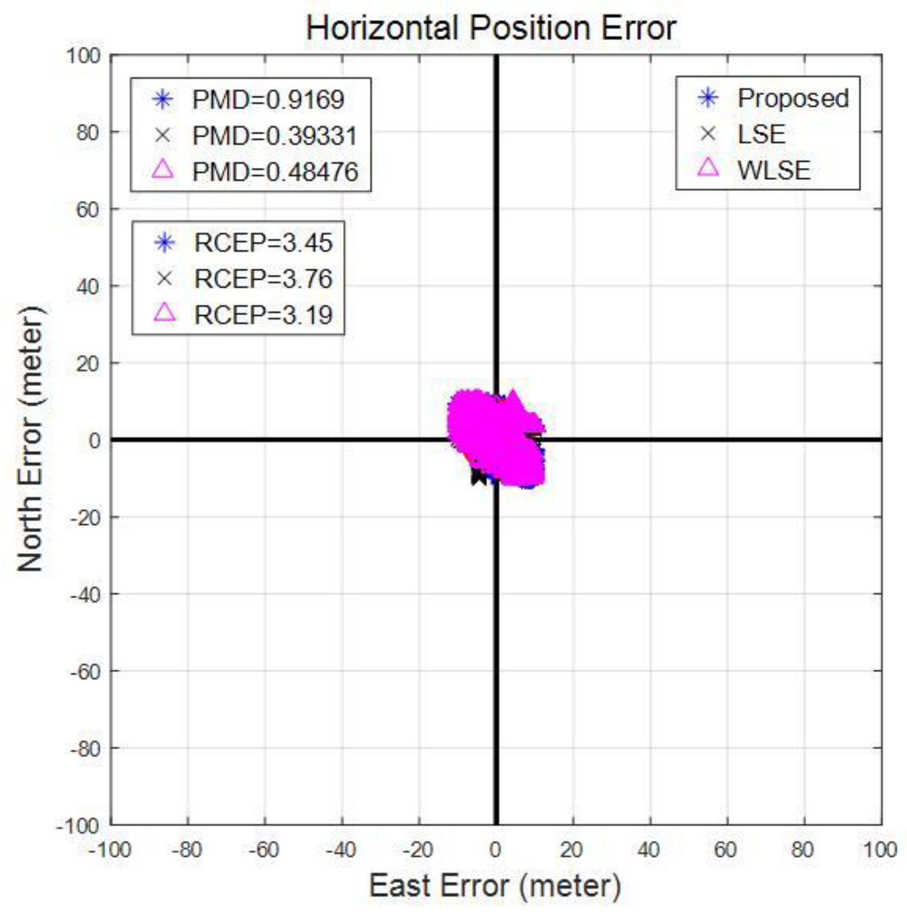
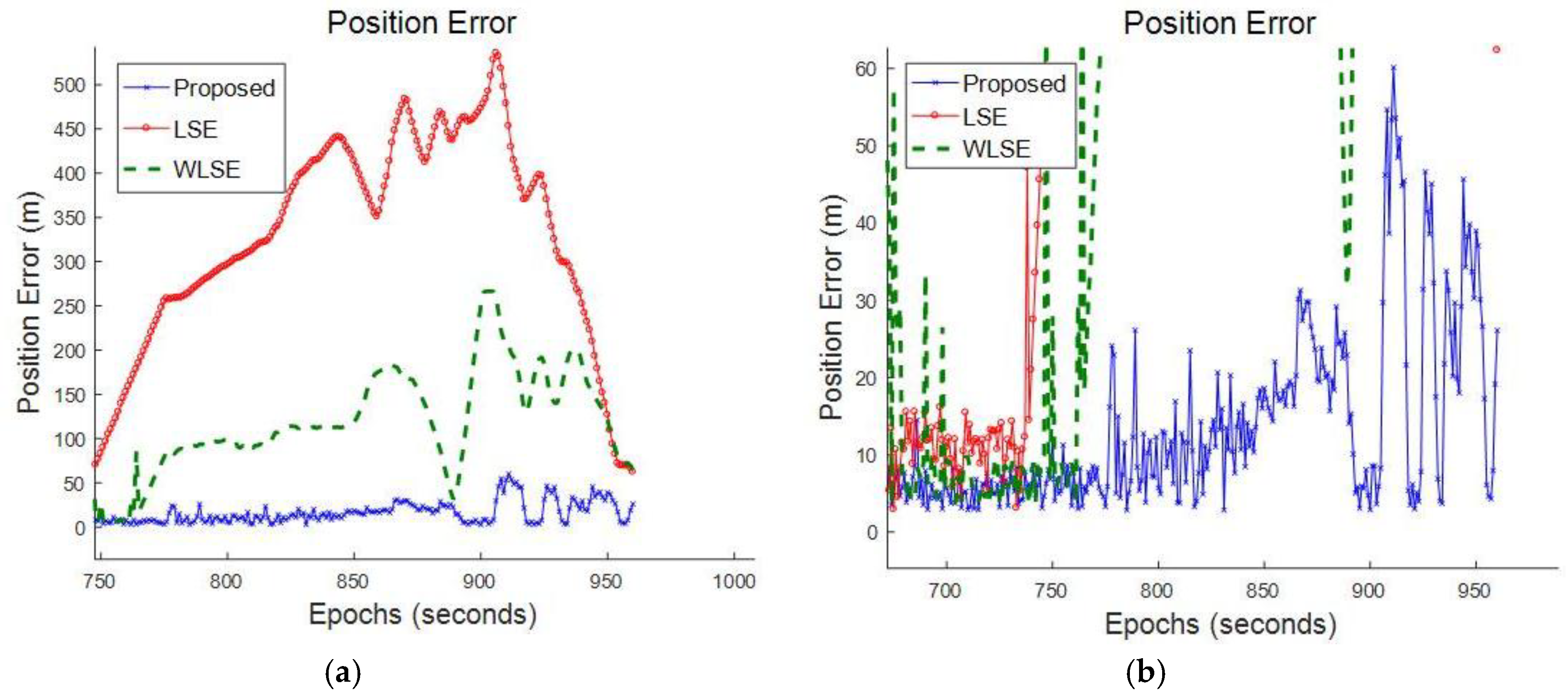
| Algorithm | LSE | WLSE | Proposed | |
|---|---|---|---|---|
| Error | ||||
| min | 1.4615 | 3.3358 | 2.6673 | |
| max | 535.8151 | 266.4498 | 94.1103 | |
| mean | 111.6460 | 39.3734 | 10.7022 | |
| std | 144.4107 | 54.1297 | 11.8657 | |
| RMS | 182.5304 | 66.9329 | 15.9787 | |
© 2018 by the authors. Licensee MDPI, Basel, Switzerland. This article is an open access article distributed under the terms and conditions of the Creative Commons Attribution (CC BY) license (http://creativecommons.org/licenses/by/4.0/).
Share and Cite
Akram, M.A.; Liu, P.; Wang, Y.; Qian, J. GNSS Positioning Accuracy Enhancement Based on Robust Statistical MM Estimation Theory for Ground Vehicles in Challenging Environments. Appl. Sci. 2018, 8, 876. https://doi.org/10.3390/app8060876
Akram MA, Liu P, Wang Y, Qian J. GNSS Positioning Accuracy Enhancement Based on Robust Statistical MM Estimation Theory for Ground Vehicles in Challenging Environments. Applied Sciences. 2018; 8(6):876. https://doi.org/10.3390/app8060876
Chicago/Turabian StyleAkram, Muhammad Adeel, Peilin Liu, Yuze Wang, and Jiuchao Qian. 2018. "GNSS Positioning Accuracy Enhancement Based on Robust Statistical MM Estimation Theory for Ground Vehicles in Challenging Environments" Applied Sciences 8, no. 6: 876. https://doi.org/10.3390/app8060876
APA StyleAkram, M. A., Liu, P., Wang, Y., & Qian, J. (2018). GNSS Positioning Accuracy Enhancement Based on Robust Statistical MM Estimation Theory for Ground Vehicles in Challenging Environments. Applied Sciences, 8(6), 876. https://doi.org/10.3390/app8060876