Multi-UAVs Communication-Aware Cooperative Target Tracking

Abstract

A kind of communication-aware cooperative target tracking algorithm is proposed, which is based on information consensus under multi-Unmanned Aerial Vehicles (UAVs) communication noise. Each UAV uses the extended Kalman filter to predict target movement and get an estimation of target state. The communication between UAVs is modeled as a signal to noise ratio model. During the information fusion process, communication noise is treated as a kind of observation noise, which makes UAVs reach a compromise between observation and communication. The classical consensus algorithm is used to deal with observed information, and consistency prediction of each UAV’s target state is obtained. Each UAV calculates its control inputs using receding horizon optimization method based on consistency results. The simulation results show that introducing communication noise can make UAVs more focused on maintaining good communication with other UAVs in the process of target tracking, and improve the accuracy of cooperative target tracking.

1. Introduction

In recent years, UAVs (Unmanned Aerial Vehicles) are playing an increasingly important role in collaborative investigation, battlefield combat, target status monitoring and other fields [1,2,3]. One of the most popular area is the multi-UAVs cooperative target tracking problem which can be abstracted as a mobile sensor network configuration problem [4,5,6,7,8]. The optimal sensor configuration can greatly reduce uncertainty of target state estimation. In the traditional target tracking problem, communication between sensors (or UAVs) usually uses the disc model [3], which means that the UAV has a clear communication radius. But the real communication between UAVs is very complicated. The disc model is only an ideal model, which cannot be a good simulation model of real communication. There have been some researches on target tracking problem with communication awareness [9,10,11,12], but the communication models ignore the impact of interference and attenuation. In reality, quality of communication is affected by many factors. There are many characteristics of the wireless channel of networked UAVs, such as signal-to-noise ratio (SNR) [9,11,12], signal-to-interference-plus-noise ratio (SINR) [13,14], and throughput gains [15,16,17,18,19]. SINR is widely used to describe the quality of a transmission in presence of interference. In order to improve the network performance using UAVs as flying base stations in a device-to-device communication network, SINR model was used in Reference [13] to quantify communication quality. In Reference [14], the authors studied a cellular-enabled UAV communication system consisting of one UAV and multiple GBSs (ground base stations). The quality of GBS-UAV link was determined by the received SNR. A similar problem was also studied in Reference [15], where an UAV was dispatched as a mobile AP (access point) in an UAV-enabled wireless powered communication network. The work in Reference [16] considered a new method maximizing the minimum throughput over all ground users to optimize UAV trajectory in a wireless network. In Reference [17], to optimize the performance of UAV-based wireless systems in terms of the average number of bits transmitted to users, a framework was proposed to get a better communication between UAVs. In Reference [18], a novel framework was proposed to enable reliable uplink communication for IoT (Internet of Things) devices with a minimum total transmit power. The authors in Reference [19] proposed a new hybrid network architecture by leveraging the use of UAV as a mobile base station to help offloading traffic from GBSs. In these works, the quality of communication was essential and well modeled. However, it was difficult for us to use these models in the cooperative target tracking problem since we required to reach a compromise between observation and communication. The method proposed in Reference [9] raised a communication probability model calculating the probability of successful information transmission between UAVs according to the signal-to-noise ratio. This probability and information was used to calculate UAV expected information, which could be used as criterion for maneuver decision-making. This probability model could partly reflect the influence of UAVs communication on expected information, but could not reflect real conditions of communication. In reality, information transmission is not just successful or not; there may be interference from the environment or other UAVs. In order to describe the communication in a better way, the concept of “communication noise” was raised in Reference [11]. However, the observation model in Reference [11] was overly simplified. In addition, UAVs need to predict link qualities, which may be not practical in the real world because of deep fades. In this paper, we use the concept of communication noise and propose a new method to get control input for each UAV. The results based on communication probability model and communication noise model in this paper are compared. The results show that the proposed method is superior to the communication probability model in terms of target state estimation.

2. Problem Description and System Model

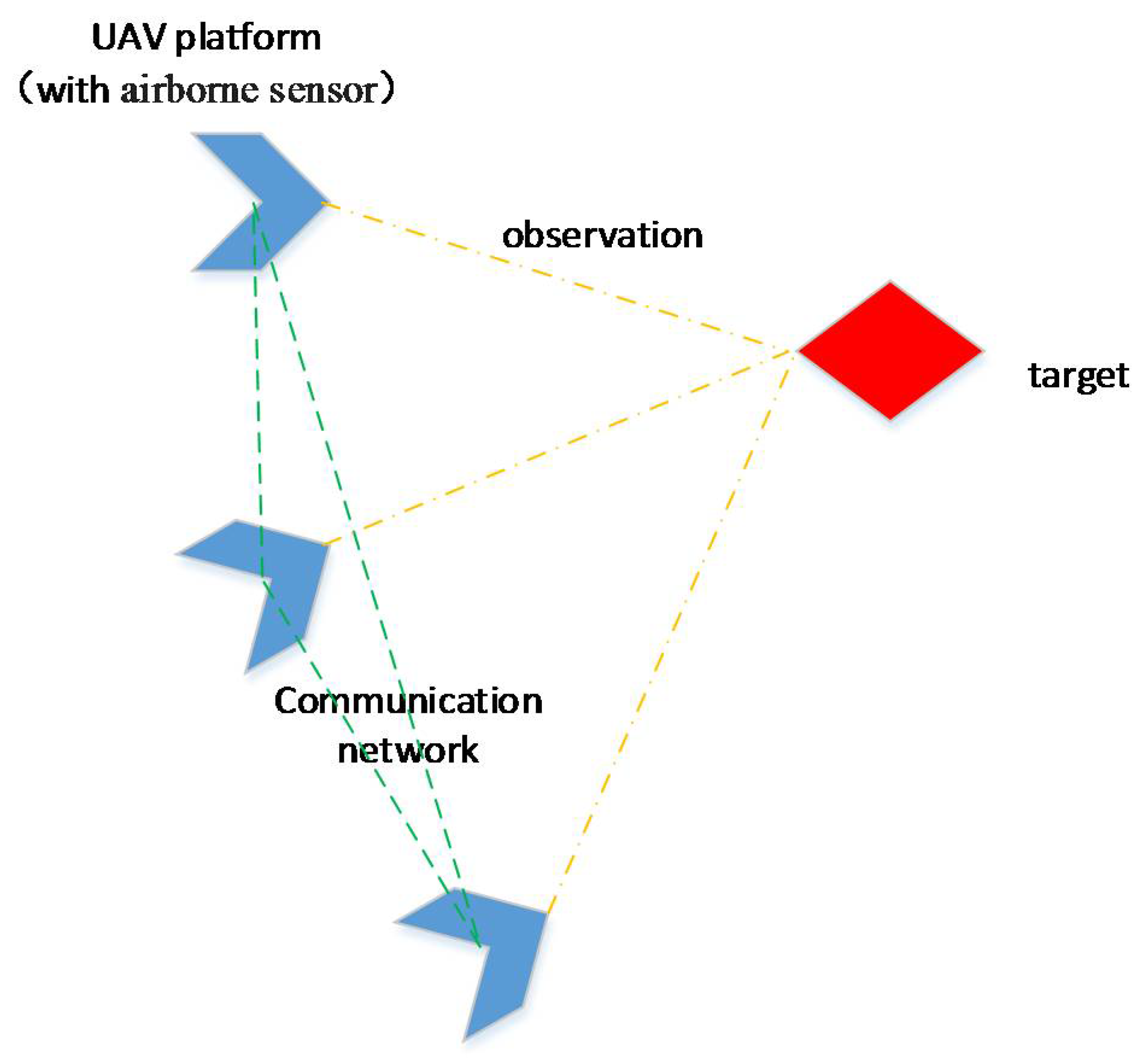
Multi-UAVs cooperative target tracking problem is shown in Figure 1. A target moves on the ground while several UAVs track it cooperatively. Each UAV is equipped with an airborne sensor and a local filter to get a better estimation of the target state. Since the sensor is not perfect, it has an observation noise so it may also need information from other UAVs. Thus, each UAV platform receives information from its neighbors (we define “neighbor” in Section 2.3) and in the meanwhile shares its information with them. Observation information from neighbor nodes contain communication noise. Each UAV will run the information fusion and the consistent process to make use of other UAVs’ information in order to get a consistent target state prediction, which is used to calculate each UAV’s control input. In this paper, the target tracking problem involves three kinds of noise: Process noise of target movement, observation noise of the sensor, and communication noise during communication between UAVs.

2.1. Target Motion Model

The motion of the target is shown as the following linear dynamics:

$$X_t[k+1]=F_{cv}{X}_t[k]+G_{cv}\rho [k]$$

(1)

where $F_{cv}$ is the state transition matrix:

$$F_{cv}=\left[\begin{array}{cccc}1& 0& \Delta T& 0\\ 0& 1& 0& \Delta T\\ 0& 0& 1& 0\\ 0& 0& 0& 1\end{array}\right] \mathrm{and}$$

(2)

$G_{cv}$ is the noise input matrix:

$$G_{cv}=\left[\begin{array}{cc}\frac{1}{2}\Delta T^2& 0\\ 0& \frac{1}{2}\Delta T^2\\ \Delta T& 0\\ 0& \Delta T\end{array}\right]$$

(3)

In Equation (1), $X_t={[x_t,y_t,{\dot{x}}_t,{\dot{y}}_t]}^T$ represents the target state, including location and speed. $\rho ={[{\rho }_{vx},{\rho }_{vy}]}^T$ represents the process noise. ${\rho }_{vx}$ and ${\rho }_{vy}$ are assumed as Gaussian and white noise with zero mean. $\rho \sim N(0,Q)$ with Q: Covariance matrix of process noise.

2.2. Observation Model

Usually, each UAV is equipped with a local sensor such as radar, infrared sensor, or a camera. With the development of sensor technology, some of the most advanced sensor devices, such as SAR/GMTI radar and ESM, have gradually been installed on small and medium-sized UAV platforms. This paper mainly considers direction-finding sensors represented by photoelectric/infrared imaging sensors, ranging sensors represented by ultrasonic/laser radar, and a combination of both. Additionally, this paper focuses on how to maintain a stable tracking of the target in presence of noise in target information, rather than studying the sensor itself.

We assume that the UAVs’ flight altitude remains the same. Then, the UAVs and the target can be projected onto horizon for analysis. Doing so, a simplified airborne sensor observation model can be obtained as shown in Equation (4).

$$z_i=\left[\begin{array}{l}{r}_i\\ {\phi }_i\end{array}\right]=h(X_t)=\left[\begin{array}{l}\sqrt{{(x_i-x_t)}^2+{(y_i-y_t)}^2}\\ \arctan \frac{y_i-y_t}{x_i-x_t}\end{array}\right]+\left[\begin{array}{l}{\upsilon }_{r,i}\\ {\upsilon }_{\phi ,i}\end{array}\right]$$

(4)

where $r_i$ is the distance between the i-th UAV and the target, ${\phi }_i$ the angle between the i-th UAV and the target, and $h(·)$ the observation function. ${\upsilon }_i$ represents the observation noise, and ${\upsilon }_i=\left[\begin{array}{l}{\upsilon }_{r,i}\\ {\upsilon }_{\phi ,i}\end{array}\right]\sim N(0,R_i)$ in which $R_i$ is the covariance matrix. Usually, for the safety of UAV as well as the need of target tracking, an UAV is not supposed to be too close to the target, which we call a minimum observation distance.

2.3. Communication Model

In the traditional cooperative tracking algorithm, the widely used communication model is the “disk model”. The disk model assumes that there is a clear communication distance d between UAVs. If the distance of two UAVs is less than d, communication between them is 100% successful; otherwise, they cannot communicate with each other. The model is an ideal model which does not take the complexity of actual communication into account. When we studied UAVs network topology [20], this model could be used to simplify the problem, but when we estimated the target state in the target tracking problem, the disk model could not meet the accuracy requirements. Therefore, this paper introduces communication noise, based on communication signal to noise ratio, so it can be compared with the observed noise covariance and process noise covariance.

There are several methods to handle communication between UAVs. The method proposed in Reference [9] took the reliability of multi-hop networked communication into account. It built a function of SNR to describe the probability of communication between node i and node j and then established an objective function with the expected value. The work in Reference [11] considered real communication and proposed the concept of “communication noise” to describe communication between two UAVs. In this paper, we used the concept of communication noise and applied the form of Fisher information matrix (FIM) to add communication noise to the objective function. Then, we proposed a new method to put communication noise into the FIM and get control input for each UAV.

A local filter was designed for each UAV platform (the extended Kalman filter is used in this paper) to get a better estimate of the target state. ${\widehat{x}}_i[k],e_i[k],P_i[k]$ represents the state estimate of the i-th UAV, its corresponding estimate errors, and its error co-variance matrix, respectively. Each UAV sends the estimated value of the target state and its corresponding covariance matrix to its neighbors. ${\widehat{x}}_{j,i}[k]$ represents the reception value of the i-th UAV from the j-th UAV and $P_{j,i}[k]$ the corresponding covariance matrix:

$$\begin{array}{l}{\widehat{x}}_{j,i}[k]={\widehat{x}}_j[k]+c_{j,i}[k]\\ P_{j,i}[k]=P_j[k]+L_{j,i}[k]\end{array}$$

(5)

where $c_{j,i}[k]$ and $L_{j,i}[k]$ contain the error and its corresponding covariance matrix caused by communication noise [11]. The communication noise covariance matrix can be calculated with the following Equation (6):

$${\displaystyle {\sum }_{{}_{j,i}}[k]}=\overline{c_{ji}[k]c_{ji}^T[k]}=\psi (SN{R}_{j,i}[k]).$$

(6)

A wireless transmission is degraded by several factors, among which distance-dependent path loss, fading, and receiver thermal noise are the most critical. One of the most fundamental parameter of a communication channel is the received signal–to–noise ratio (SNR). $SN{R}_{j,i}[k]$ represents the SNR from node j to node i at time k. We can calculate SNR with the following equation:

$$SN{R}_{j,i}[k]=\frac{Powe{r}_j\cdot Gai{n}_{ji}}{N_i}.$$

(7)

In addition, for a distance-dependent path loss without fading, we have:

$$Gai{n}_{ji}=\frac{C_{ji}{|h_{ji}[k]|}^2}{d_{ji}^{n_p}}$$

(8)

where $Powe{r}_j$ in (7) represents the transmission signal power, $N_i={\sigma }_T^2=E({|n_{thermal}|}^2)$ the noise power at the receiver, $Gai{n}_{ji}$ the channel gain, $h_{j,i}[k]$ the attenuation factor for the communication environment, $d_{ji}^{}$ the distance between the i-th UAV and the j-th UAV, and $C_{ji}$ the communication environment impact factor. SNR determines the effectiveness of communication.

Then, we can rewrite Equation (7) as the following:

$$\begin{array}{l}SN{R}_{j,i}[k]=\frac{{\alpha }_{ji}[k]}{d_{ji}^{n_p}[k]}\\ {\alpha }_{ji}[k]=\frac{Powe{r}_j{C}_{ji}{|h_{ji}[k]|}^2}{N_i}\end{array}$$

(9)

where ${\alpha }_{ji}[k]$ is an intermediate variable.

In a fading environment, however, the SNR is a random variable. We followed the same model used in References [11,21]:

$$SN{R}_{j,i,ave}[k]=E(SN{R}_{j,i,fading}[k])=\frac{{\alpha }_{ji}[k]}{d_{ji}^{n_p}[k]}$$

(10)

where $SN{R}_{j,i,ave}[k]$ is the average of fading and $SN{R}_{j,i,fading}[k]$ the SNR in the presence of fading. More information can be found in Reference [21].

In order to make sure that node i can successfully receive information sent by node j with a small packet loss probability, SNR at node i is required to be greater than a threshold value $\gamma$. Therefore, if the SNR of node i from node j is greater than $\gamma$, node j is one of node i’s neighbors. An UAV can communicate with its neighbors.

$c^{(1)}{}_{j,i}[k]$ and ${\mathrm{\Sigma }}_{j,i}^{(1,1)}[k]$ represent the communication noise of $r_j$ and its corresponding covariance matrix from the j-th UAV to the i-th UAV. From Equation (6) we can get:

$${\mathrm{\Sigma }}_{j,i}^{(1,1)}[k]=\mathrm{E}({|c_{j,i}^{(1)}[k]|}^2|h_{j,i}[k])$$

(11)

$${\mathrm{\Sigma }}_{j,i}^{(1,1)}[k]={\psi }^{(1,1)}(SN{R}_{j,i}[k])$$

(12)

where $\psi (·)$ can be determined as:

$${\mathrm{\Sigma }}_{j,i}^{(1,1)}[k]={\psi }^{(1,1)}(SN{R}_{j,i}[k])=\frac{q^2}{12}+\frac{4^{Nb}-1}{3}{q}^2\times \mathrm{\Omega }(\sqrt{SN{R}_{j,i}[k]})$$

(13)

where

$$\mathrm{\Omega }(\eta )=\frac{1}{\sqrt{2\pi }}{\displaystyle {\int }_{\eta }^{\infty }{e}^{-z^2/2}dz}.$$

(14)

Similarly, the communication noise variance can be obtained with respect to ${\phi }_j$. Readers are referred to Reference [21] for more details.

Besides the attenuation of a wireless channel, we should also consider the impact of interference between UAVs. In this paper, we used the signal-to-interference-plus-noise ratio (SINR) [13,17] to describe it. The SINR expression for a receiver is:

$$SIN{R}_{j,i}[k]=\frac{Powe{r}_j\cdot G_{ji}}{N_i+{\mathrm{I}}_{ji}[k]}$$

(15)

where ${\mathrm{I}}_{ji}[k]$ is the received interference of UAV i stemming from UAV j.

We can replace SNR with SINR if it is needed in Equation (9) or Equation (12).

2.4. UAV Motion Model

We used the following UAV motion model:

$$\left[\begin{array}{l}{\dot{x}}_i\\ {\dot{y}}_i\\ {\dot{\phi }}_i\end{array}\right]=\left[\begin{array}{l}{v}_i\cos {\phi }_i\\ v_i\sin {\phi }_i\\ {\alpha }_{\phi }({\phi }_i^c-{\phi }_i)\end{array}\right]$$

(16)

s.t.

$$-{\omega }_{\max }\le {\dot{\phi }}_i\le {\omega }_{\max }.$$

(17)

$X_i={[x_i,y_i,{\phi }_i]}^T$ is the state of UAV, in which $(x_i,y_i)$ is the position and ${\phi }_i$ the heading angle. In this paper, the speed of UAV is constant. ${\alpha }_{\phi }$ is the heading gain, ${\phi }_i^c$ the control input which represents the expected heading angle, and ${\omega }_{\max }$ the maximum angular velocity.

3. Information Fusion Based on Extended Information Filtering

In the process of cooperative target tracking for UAVs, each UAV needs to make a precise estimation of the state of the moving target in order to calculate the control input in real-time. Because of the non-linearity of the observation model, the traditional Kalman filter cannot be qualified for the filtering process, so other filtering methods are needed. Generally speaking, the extended Kalman filter [22], unscented Kalman filter [12,22], and particle filter [23] are widely used to solve the nonlinearity of the system model problem [3]. In this paper, extended Kalman filter was used.

Time update process of extended Kalman filter:

$${\widehat{X}}_k^{-}=F_{cv}{\widehat{X}}_k^{}$$

(18)

$$P_k^{-}=F_{cv}{P}_i{F}_{cv}^T+Q_k.$$

(19)

Measurement update process of extended Kalman filter:

$$K_k=P_k^{-}{H}_k^T({\widehat{X}}_k^{-}){[H_k({\widehat{X}}_k^{-})P_k^{-}{H}_k^T({\widehat{X}}_k^{-})+R_k]}^{-1}$$

(20)

$${\widehat{X}}_k={\widehat{X}}_k^{-}+K_k[z_k-h({\widehat{X}}_k^{-})]$$

(21)

$$P_k=P_k^{-}-K_k{H}_k({\widehat{X}}_k^{-})P_k^{-}$$

(22)

where $h(·)$ is the corresponding function of the observation Equation (4), $H_k(·)$ the Jacobian matrix of $h(·)$, $F_{cv}$ the transition matrix of the target, ${\widehat{X}}_k^{-}$ the predicted target state at time k, ${\widehat{X}}_k$ the estimated target state at time k, $Q_k$ the covariance matrix of the process noise at time k, $R_k$ the covariance matrix of the observation noise at time k, $P_k^{-}$ the covariance matrix of the predicted target state, $P_k$ the covariance matrix of the estimated target state, and $K_k$ the gain matrix of Kalman filter.

3.1. Extend Information Filter and Information Fusion Phase

Fisher’s information matrix is a way of describing target state estimation and is widely used in the optimal estimation theory [3,11]. It can be very convenient to do information fusion using fisher information matrix (FIM). For i-th UAV, the Fisher information matrix is defined as follows:

$$Y_i[k]=P_i{}^{-1}[k]$$

(23)

$$y_i[k]=Y_i[k]{\widehat{X}}_i[k]$$

(24)

where $Y_i[k]$ represents the information matrix at time k, $y_i[k]$ the information state matrix, and $P_i$ the matrix $P_k$ in Equation (22). For the observed value $z[k]$ at the discrete time k, its gain for the information matrix and the information state matrix are:

$$\begin{array}{l}{I}_i[k]=H^T[k]R^{-1}[k]H[k]\\ i_i[k]=H^T[k]R^{-1}[k]z[k]\end{array}.$$

(25)

Combined with Equations (23)–(25) and Equations (18)–(22), we get:

$$\begin{array}{l}{Y}_i{}^{{}^s-}[k]={(P_i^{-})}^{-1}\\ {\widehat{y}}_i{}^{s-}[k]=Y_i{}^{-}[k]{\widehat{X}}_i[k-1]\end{array}$$

(26)

$$\begin{array}{l}{I}^s{}_i[k]=H^T[k]R^{-1}[k]H[k]\\ i^s{}_i[k]=H^T[k]R^{-1}[k]z[k]\end{array}$$

(27)

$$\begin{array}{l}{Y}_i{}^s[k]=Y_i{}^{-}[k]+I_i[k]\\ {\widehat{y}}^s{}_i[k]={\widehat{y}}_i{}^{-}[k]+i_i[k]\end{array}.$$

(28)

The superscript “s” represents the information matrix before performed information fusion. It can be seen that the Fisher information matrix can easily superimpose the observation results into the information matrix through the information gain matrix, and this greatly reduces the computational complexity in the process of multi-UAVs information fusion.

The posteriori state estimation can be obtained from Equation (29):

$${\widehat{x}}_i[k]=Y^{-1}[k]\widehat{y}[k].$$

(29)

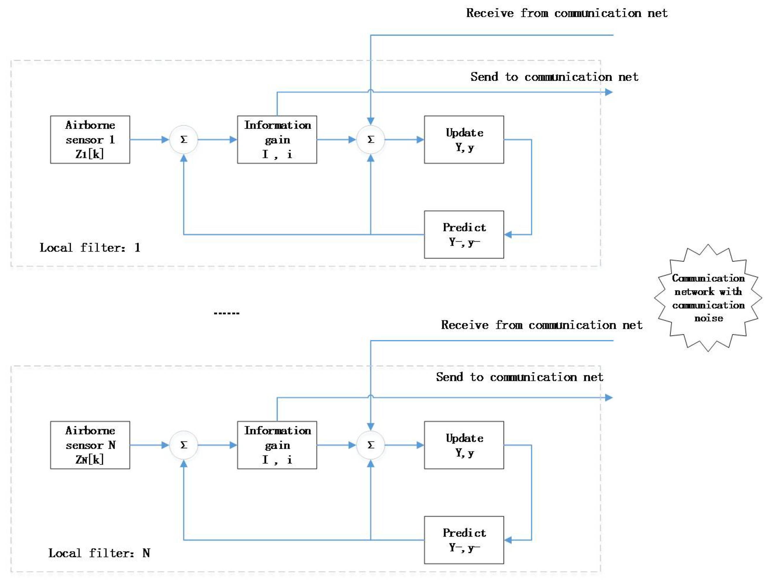
Assuming that the observation of each UAV airborne sensors is not relevant, we can get the information fusion process shown in Figure 2.

In the process of information fusion with communication noise, communication noise changes the gain matrix of information transmitted by other UAVs. For the i-th UAV, the information matrix $Y_i$ and the information state matrix of the target state ${\widehat{y}}_i$ can be rewritten as:

$$Y_i[k]=Y_i^s[k]+{\displaystyle \sum _{j\ne i}{I}_{ji}^c}[k]$$

(30)

$${\widehat{y}}_i[k]={\widehat{y}}_i^s[k]+{\displaystyle \sum _{j\ne i}{i}_{ji}^c[k]}$$

(31)

where $Y_i^s[k]$, ${\widehat{y}}_i[k]$ represent the information matrix and information state matrix from the i-th UAV, which can be calculated using Equation (28). $I_{j,i}^c[k]$, $i_{ji}^s[k]$ represent information gain matrix and information state gain matrix from the j-th UAVs to the i-th UAV. In the presence of communication noise, according to Equation (27), $I_{j,i}^c[k]$ and $i_{ji}^c[k]$ can be calculated using Equations (32) and (33).

$$I_{j,i}^c[k]=H_j{}^T[k]{(R_j+{\mathrm{\Sigma }}_{ji}[k])}^{-1}{H}_j[k]$$

(32)

$$i_{j,i}^c[k]=H_j{}^T[k]{(R_j+{\mathrm{\Sigma }}_{ji}[k])}^{-1}{z}_j[k]$$

(33)

where ${\mathrm{\Sigma }}_{j,i}[k]$ represents communication noise covariance matrix from the j-th UAVs to the i-th UAV and can be calculated using Equations (11)–(14). From Equations (30)–(33), we get

$$Y_i[k]=Y_i^s[k]+{\displaystyle \sum _{j\ne i}{H}_j{}^T[k]{(R_j+{\mathrm{\Sigma }}_{ji}[k])}^{-1}{H}_j[k]}$$

(34)

$${\widehat{y}}_i[k]={\widehat{y}}_i^s[k]+{\displaystyle \sum _{j\ne i}{H}_j{}^T[k]{(R_j+{\mathrm{\Sigma }}_{ji}[k])}^{-1}{z}_j[k]}.$$

(35)

With Equations (30) and (32) we get:

$$\begin{array}{l}{Y}_i[k]=Y_i^s[k]+{\displaystyle \sum _{j\ne i}{H}_j{}^T[k]{(R_j+{\mathrm{\Sigma }}_{ji}[k])}^{-1}{H}_j[k]}\\ \begin{array}{cc}\begin{array}{cc}& \end{array}& =\end{array}{Y}_i^{s-}[k]+I_i^s+{\displaystyle \sum _{j\ne i}\left\{I_j^s+H_j{}^T[k]{({\mathrm{\Sigma }}_{ji}[k])}^{-1}{H}_j[k]\right\}}\\ \begin{array}{cc}\begin{array}{cc}& \end{array}& =\end{array}\underset{local-estimate}{\underbrace{Y_i^{s-}[k]}}+\underset{observation}{\underbrace{{\displaystyle \sum _{}{I}_j^s}}}+\underset{communication-noise}{\underbrace{{\displaystyle \sum _{j\ne i}{\mathrm{\Gamma }}_{ji}^c}}}\end{array}$$

(36)

where

$${\mathrm{\Gamma }}_{ji}^c=H_j{}^T[k]{({\mathrm{\Sigma }}_{ji}[k])}^{-1}{H}_j[k].$$

(37)

From Equation (34) we can figure out that in this paper, the communication noise was treated as a kind of observation noise from others. Equation (34) can be written as Equation (36), which is different from the method proposed in Reference [11]. It makes UAVs reach a compromise between observation and communication, and track the target cooperatively.

Similar expression can be written for ${\widehat{y}}_i[k]$. Then, we can use the determinant of $Y_i[k]$ as the objective function for each UAV, which can be found in Section 4.

Next, we give a mathematical proof for our method to explain how it works when we put communication noise into the objective function, and to prove how our proposed method finds a way to reach a compromise between observation and communication for each UAV. Firstly, we give the following definition:

$$N_i\triangleq the\hspace{0.17em}set\hspace{0.17em}of\hspace{0.17em}UAV\hspace{0.17em}i\prime s\hspace{0.17em}neighbours(without\hspace{0.17em}i)$$

$$N_i^{+}\triangleq the\hspace{0.17em}set\hspace{0.17em}of\hspace{0.17em}UAV\hspace{0.17em}i\prime s\hspace{0.17em}neighbours(including\hspace{0.17em}i)$$

$$R_i=\left[\begin{array}{l}\begin{array}{cc}{\sigma }_r^2& \hspace{1em}\end{array}\\ \begin{array}{cc}\hspace{1em}& {\sigma }_{\phi }^2\end{array}\end{array}\right]$$

(38)

$${\displaystyle \sum {}_{ji}=}\left[\begin{array}{cc}\begin{array}{c}{c}_{rj}^2\\ \end{array}& \begin{array}{c}\\ c_{\phi j}^2\end{array}\end{array}\right]\triangleq \left[\begin{array}{cc}\begin{array}{c}{({\mathrm{\Sigma }}_{ji}^{1,1})}^2\\ \end{array}& \begin{array}{c}\\ {({\mathrm{\Sigma }}_{ji}^{2,2})}^2\end{array}\end{array}\right]$$

(39)

$${\tilde{J}}_i\triangleq I_i+{\displaystyle \sum _{j\in N_i}{I}_{ji}^c}.$$

(40)

Using Equations (25) and (32), we get the following expression:

$$\begin{array}{l}{\tilde{J}}_i=I_i+{\displaystyle \sum _{j\in N_i}{I}_{ji}^c}={\displaystyle \sum _{j\in N_i^{+}}}{I}_{ji}^c\\ ={\displaystyle \sum _{j\in N_i^{+}}}\left[\begin{array}{cccc}\frac{{\sin }^2{\phi }_j}{{\sigma }_r^2+c_{rj}^2}+\frac{{\cos }^2{\phi }_j}{r_j^2({\sigma }_{\phi }^2+c_{\phi j}^2)}& \frac{\cos {\phi }_j\sin {\phi }_j}{{\sigma }_r^2+c_{rj}^2}-\frac{\cos {\phi }_j\sin {\phi }_j}{r_j^2({\sigma }_{\phi }^2+c_{\phi j}^2)}& 0& 0\\ \frac{\cos {\phi }_j\sin {\phi }_j}{{\sigma }_r^2+c_{rj}^2}-\frac{\cos {\phi }_j\sin {\phi }_j}{r_j^2({\sigma }_{\phi }^2+c_{\phi j}^2)}& \frac{{\cos }^2{\phi }_j}{{\sigma }_r^2+c_{rj}^2}+\frac{{\sin }^2{\phi }_j}{r_j^2({\sigma }_{\phi }^2+c_{\phi j}^2)}& 0& 0\\ 0& 0& 0& 0\\ 0& 0& 0& 0\end{array}\right]\end{array}$$

(41)

where $c_{rj}=c_{\phi j}=0$ when j = i, which means there is no communication noise when an UAV communicates with itself.

$$J_i\triangleq {\displaystyle \sum _{j\in N_i^{+}}\left[\begin{array}{cc}\frac{{\sin }^2{\phi }_j}{{\sigma }_r^2+c_{rj}^2}+\frac{{\cos }^2{\phi }_j}{r_j^2({\sigma }_{\phi }^2+c_{\phi j}^2)}& \frac{\cos {\phi }_j\sin {\phi }_j}{{\sigma }_r^2+c_{rj}^2}-\frac{\cos {\phi }_j\sin {\phi }_j}{r_j^2({\sigma }_{\phi }^2+c_{\phi j}^2)}\\ \frac{\cos {\phi }_j\sin {\phi }_j}{{\sigma }_r^2+c_{rj}^2}-\frac{\cos {\phi }_j\sin {\phi }_j}{r_j^2({\sigma }_{\phi }^2+c_{\phi j}^2)}& \frac{{\cos }^2{\phi }_j}{{\sigma }_r^2+c_{rj}^2}+\frac{{\sin }^2{\phi }_j}{r_j^2({\sigma }_{\phi }^2+c_{\phi j}^2)}\end{array}\right]}.$$

(42)

We defined det(J) as the determinant of J. Then, from Equation (42) we get:

$$\begin{array}{l}\det (J_i)=\det \left\{{\displaystyle \sum _{j\in N_i^{+}}\left[\begin{array}{cc}\frac{{\sin }^2{\phi }_j}{{\sigma }_r^2+c_{rj}^2}+\frac{{\cos }^2{\phi }_j}{r_j^2({\sigma }_{\phi }^2+c_{\phi j}^2)}& \frac{\cos {\phi }_j\sin {\phi }_j}{{\sigma }_r^2+c_{rj}^2}-\frac{\cos {\phi }_j\sin {\phi }_j}{r_j^2({\sigma }_{\phi }^2+c_{\phi j}^2)}\\ \frac{\cos {\phi }_j\sin {\phi }_j}{{\sigma }_r^2+c_{rj}^2}-\frac{\cos {\phi }_j\sin {\phi }_j}{r_j^2({\sigma }_{\phi }^2+c_{\phi j}^2)}& \frac{{\cos }^2{\phi }_j}{{\sigma }_r^2+c_{rj}^2}+\frac{{\sin }^2{\phi }_j}{r_j^2({\sigma }_{\phi }^2+c_{\phi j}^2)}\end{array}\right]}\right\}\\ =\det \left\{{\displaystyle \sum _{j\in N_i^{+}}\left[\begin{array}{cc}\frac{1-\cos 2{\phi }_j}{2({\sigma }_r^2+c_{rj}^2)}+\frac{1+\cos 2{\phi }_j}{2r_j^2({\sigma }_{\phi }^2+c_{\phi j}^2)}& \frac{\sin 2{\phi }_j}{2({\sigma }_r^2+c_{rj}^2)}-\frac{\sin 2{\phi }_j}{2r_j^2({\sigma }_{\phi }^2+c_{\phi j}^2)}\\ \frac{\sin 2{\phi }_j}{2({\sigma }_r^2+c_{rj}^2)}-\frac{\sin 2{\phi }_j}{2r_j^2({\sigma }_{\phi }^2+c_{\phi j}^2)}& \frac{1+\cos 2{\phi }_j}{2({\sigma }_r^2+c_{rj}^2)}+\frac{1-\sin 2{\phi }_j}{2r_j^2({\sigma }_{\phi }^2+c_{\phi j}^2)}\end{array}\right]}\right\}\\ =\frac{1}{4}·\det \left\{{\displaystyle \sum _{j\in N_i^{+}}\left[\begin{array}{cc}{B}_{\sigma j}-\cos 2{\phi }_j\cdot C_{\sigma j}& \sin 2{\phi }_j\cdot C_{\sigma j}\\ \sin 2{\phi }_j\cdot C_{\sigma j}& B_{\sigma j}+\cos 2{\phi }_j\cdot C_{\sigma j}\end{array}\right]}\right\}\\ =\frac{1}{4}\cdot {\displaystyle \sum _{j\in N_i^{+}}(B_{\sigma j}-\cos 2{\phi }_j\cdot C_{\sigma j}})\cdot {\displaystyle \sum _{j\in N_i^{+}}(B_{\sigma j}+\cos 2{\phi }_j\cdot C_{\sigma j}})-\frac{1}{4}{({\displaystyle \sum _{j\in N_i^{+}}\sin 2{\phi }_j\cdot C_{\sigma j}})}^2\\ =\frac{1}{4}\cdot {\left({\displaystyle \sum _{j\in N_i^{+}}(B_{\sigma j}})\right)}^2-{\left({\displaystyle \sum _{j\in N_i^{+}}(\cos 2{\phi }_j\cdot C_{\sigma j}})\right)}^2-{\left({\displaystyle \sum _{j\in N_i^{+}}(\sin 2{\phi }_j\cdot C_{\sigma j}})\right)}^2\end{array}$$

(43)

where

$$\begin{array}{l}{B}_{\sigma j}=\frac{1}{{\sigma }_r^2+c_{rj}^2}+\frac{1}{r_j^2({\sigma }_{\phi }^2+c_{\phi j}^2)}\\ C_{\sigma j}=\frac{1}{{\sigma }_r^2+c_{rj}^2}-\frac{1}{r_j^2({\sigma }_{\phi }^2+c_{\phi j}^2)}\end{array}.$$

(44)

Then, we get the following expression:

$$\begin{array}{cc}\hfill \det (J_i)=& \frac{1}{4}\cdot {\left({\displaystyle \sum _{j\in N_i^{+}}(\frac{1}{{\sigma }_r^2+c_{rj}^2}+\frac{1}{r_j^2({\sigma }_{\phi }^2+c_{\phi j}^2)}})\right)}^2\hfill \\ & \hspace{1em}-{\left({\displaystyle \sum _{j\in N_i^{+}}(\cos 2{\phi }_j\cdot \left(\frac{1}{{\sigma }_r^2+c_{rj}^2}-\frac{1}{r_j^2({\sigma }_{\phi }^2+c_{\phi j}^2)}\right)})\right)}^2\hfill \\ & \hspace{1em}-{\left({\displaystyle \sum _{j\in N_i^{+}}(\sin 2{\phi }_j\cdot \left(\frac{1}{{\sigma }_r^2+c_{rj}^2}-\frac{1}{r_j^2({\sigma }_{\phi }^2+c_{\phi j}^2)}\right)})\right)}^2\hfill \end{array}.$$

(45)

We can see from Equation (45) that $r_j=r_{\min }$ is a necessary condition for the maximum of $\det (J_i)$, and has an upper limit.

When $r_j=r_{\min }$ and the communication between UAVs is perfect, which means $c_{rj}=c_{\phi j}=0$, we can rewrite Equation (45) as:

$$\begin{array}{cc}\hfill \det (J_i)=& \frac{1}{4}\cdot {\left({\displaystyle \sum _{j\in N_i^{+}}(\frac{1}{{\sigma }_r^2}+\frac{1}{r_{\min }^2{\sigma }_{\phi }^2}})\right)}^2\hfill \\ & \hspace{1em}-{\left(\frac{1}{{\sigma }_r^2}-\frac{1}{r_{\min }^2{\sigma }_{\phi }^2}\right)}^2\left({\left({\displaystyle \sum _{j\in N_i^{+}}(\cos 2{\phi }_j})\right)}^2+{\left({\displaystyle \sum _{j\in N_i^{+}}(\sin 2{\phi }_j})\right)}^2\right)\hfill \end{array}.$$

(46)

Thus, when the communication is perfect, the necessary and sufficient condition to get the maximum $\det (J_i)$ is:

$${\displaystyle \sum _{j\in N_i^{+}}(\cos 2{\phi }_j})=0\hspace{0.17em}\&\hspace{0.17em}{\displaystyle \sum _{j\in N_i^{+}}(\sin 2{\phi }_j})=0.$$

(47)

Then, from Equation (47), when $N\ge 3$, we get the following observation configuration:

$${\phi }_{i,j}=\frac{2}{N}\pi$$

(48)

where ${\phi }_{i,j}$ means the angle between UAV i and j.

This is shown in Figure 3. We know from Equation (48) that when the communication is perfect, UAVs tend to be dispersed around the target to get a better observation. But, due to the communication noise between UAV i and j, using the observation configuration of Equation (48) cannot get the maximum of $\det (J_i)$, which can be seen from Equation (45). So, in order to reduce communication noise, the UAVs tend to get as close as they can. When they are getting too close, the communication noise is very low, and as a result, we can consider the communication is perfect. But from Equation (48) we can see that it is not conducive to observation when they are getting too close. Therefore, the objective function in Equation (45) can make UAVs reach a compromise between observation and communication in a natural way.

3.2. Consistence

Usually, in a distributed structure, the information matrix obtained by information fusion of each node is different. In order to ensure that the UAVs have the same environments awareness, it is necessary to use the consistency algorithm to make the information matrix tending to be consistent. In this paper, the traditional classical consistency algorithm was adopted.

The algorithm is described as follows [5,6]:

$${\xi }_i[d+1]=W_{ii}{\xi }_i[d]+{\displaystyle \sum _{j\in N_i}{W}_{ij}{\xi }_j[d]}={\xi }_i[d]+{\displaystyle \sum _{j\in N_i}{W}_{ij}({\xi }_j[d]}-{\xi }_i[d])$$

(49)

where W is the consistency weighted matrix. It can use the following expression:

$$W_{ij}=\{\begin{array}{l}{(\max \{N_i,N_j\})}^{-1},j\in N_i\\ 1-{\displaystyle \sum _{i,k\in N_i}{W}_{ik}},i=j\\ 0,otherwise\end{array}.$$

(50)

4. Distributed Motion Control Algorithm

After target state estimation and fusion based on consistency spread information filtering, each UAV can form a consistent target view; that is the target information matrix.

In this paper, the receding horizon method [2,24,25,26] was used to make maneuver decision for multi-UAVs target tracking problem. We set the length of horizon L = 3, that means, “look forward 3 steps, take one step”.

The method of finite step prediction of target state is shown in Equation (51):

$$X_{i,t}^{pred}[k+L|k]=\left[\begin{array}{c}{X}_{i,t}^{pred}[k+1|k]\\ \begin{array}{l}{X}_{i,t}^{pred}[k+2|k]\\ \dots \dots \end{array}\\ X_{i,t}^{pred}[k+L|k]\end{array}\right]=\left[\begin{array}{l}{\widehat{x}}_t^{-}[k+1|k]\\ A·{\widehat{x}}_t^{-}[k+1|k]\\ \dots \dots \\ A^{L-1}·{\widehat{x}}_t^{-}[k+1|k]\end{array}\right]$$

(51)

where $X_{i,t}^{pred}[k+L|k]$ is the L-step prediction of the target state at time k. A is the state transition matrix, in this paper, it’s $F_{cv}$.

The estimation error corresponding to Equation (51) is written as:

$$\epsilon [k+L|k]=X[k+L]-X_{i,t}^{pred}[k+L|k].$$

(52)

Thus, the covariance of the target prediction in the entire time range L is obtained:

$${\sigma }_i[k+L|k]=\left[\begin{array}{l}{\epsilon }^2[k+1|k]\\ {\epsilon }^2[k+2|k]\\ \dots \dots \\ {\epsilon }^2[k+L|k]\end{array}\right]=\left[\begin{array}{l}{(Y_i{[k+1]}^{-})}^{-1}+R\\ A{(Y_i{[k+1]}^{-})}^{-1}{A}^T+Q+R\\ \dots \dots \\ A^{L-1}{(Y_i{[k+1]}^{-})}^{-1}{(A^{L-1})}^T+Q+R\end{array}\right].$$

(53)

Then, we get the optimization function as:

$$u_i^{\ast }=arc\max \rho (Y_i(X_{i,t}^{pred}[k+L|k],u)$$

(54)

where $\rho (·)$ is the scalar function of the matrix; in this paper we used the determinant as scalar function. $X_{i,t}^{pred}[k+L|k]$ represents the prediction of target state after L steps for i-th UAV and $Y_i$ the information matrix of i-th UAV.

5. Simulation Results and Analysis

The simulation parameters were set as follows: The target initial position was (−800 m, 0 m); the target moving speed was 10 m/s; the heading was 20°; the standard deviation of the process noise was 0.1 m/s²; the speed of the UAV was 50 m/s; the standard deviation of ranging sensor was 2 m; the standard deviation of direction sensor was 0.05 rad; the angular velocity range was −30~30°/s; the safety distance between UAVs was 50 m; the horizon length taken in this paper was L = 3; and the simulation time was 100 s. The relevant parameters of the communication link model in Equations (7) and (8) are shown in

Table 1. The relevant parameters of the communication link model. SNR: signal-to-noise ratio.

Parameters	Value	Unit
$P_j$	30	dBm
$C_{ji}$	1	-
$n_p$	3	-
$\gamma$: Threshold value of SNR	10	-

.

The control decision of UAVs can be made using Equation (54) to obtain the control input for each UAV. In this paper, we used receding horizon optimization to solve the problem. The simulation results are shown in Figure 4, Figure 5, Figure 6, Figure 7, Figure 8, Figure 9, Figure 10, Figure 11 and Figure 12.

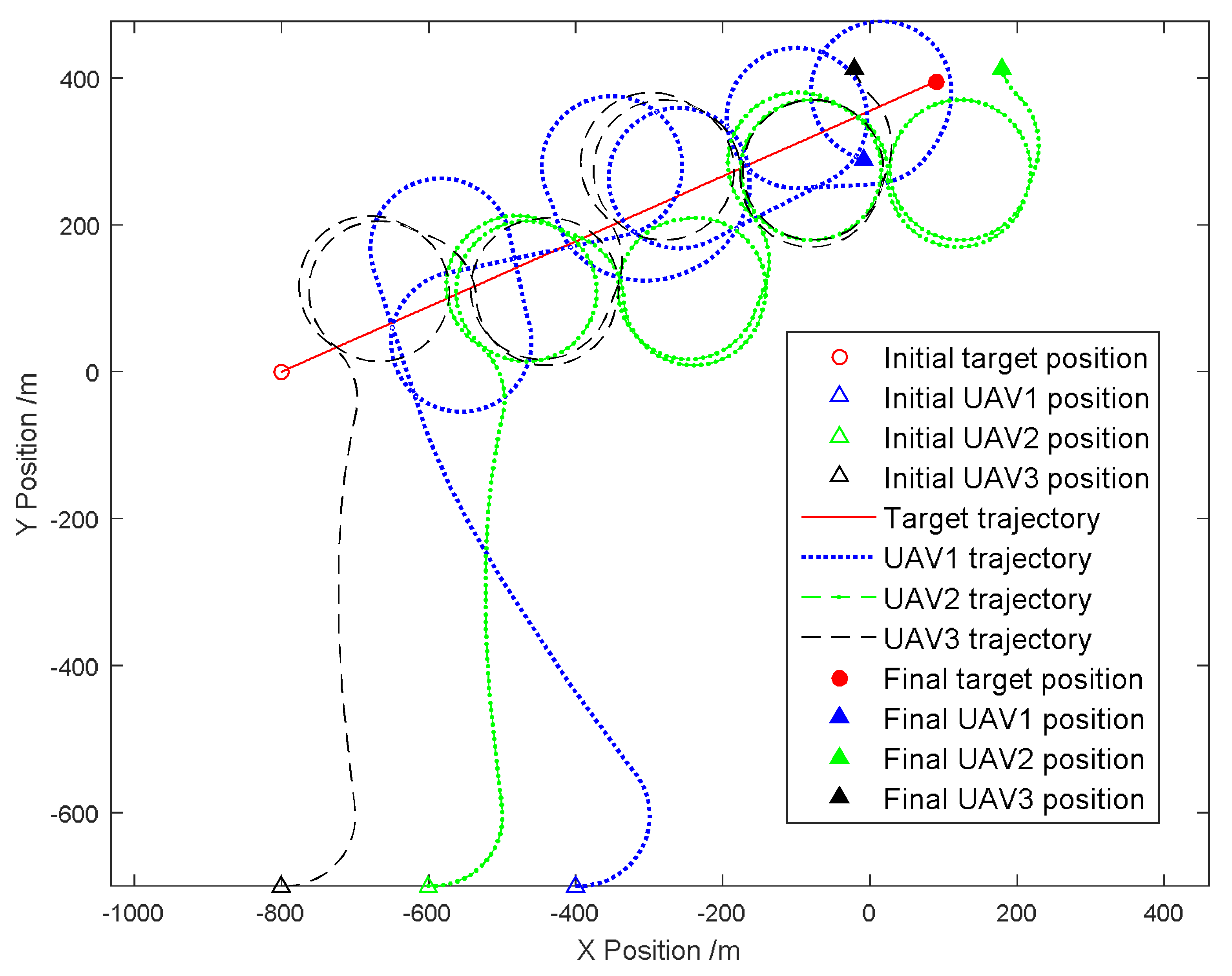
Figure 4 shows the trajectories of the target and the UAVs in one of the simulations. The initial position and the trajectory of UAVs are shown. The red solid line was the target’s trajectory and the other lines were the UAVs’ trajectory. The hollow dot and triangle represent the initial positions while the filled dot and triangle represent the final positions. We can see that at the beginning of the simulation, the UAVs got close to the target to get a better observation and then circled around it. The error of estimation is shown in Figure 5.

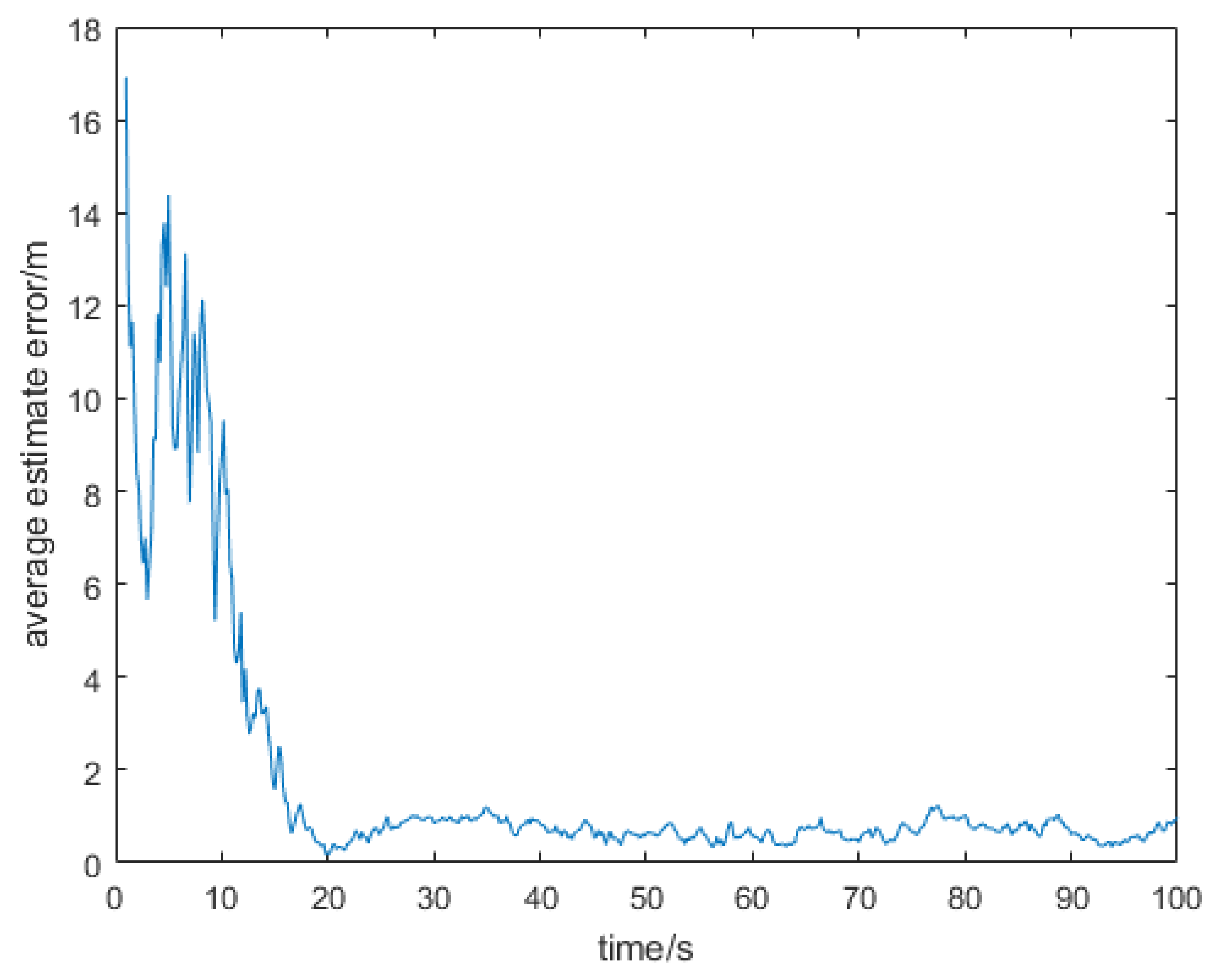
Figure 5 shows the average estimate error of the UAVs. At the beginning of the simulation, the error was large and unstable, because during this time the UAVs were too far from the target. Once they caught up the target and circled around it, the estimate error dropped quickly and became stable.

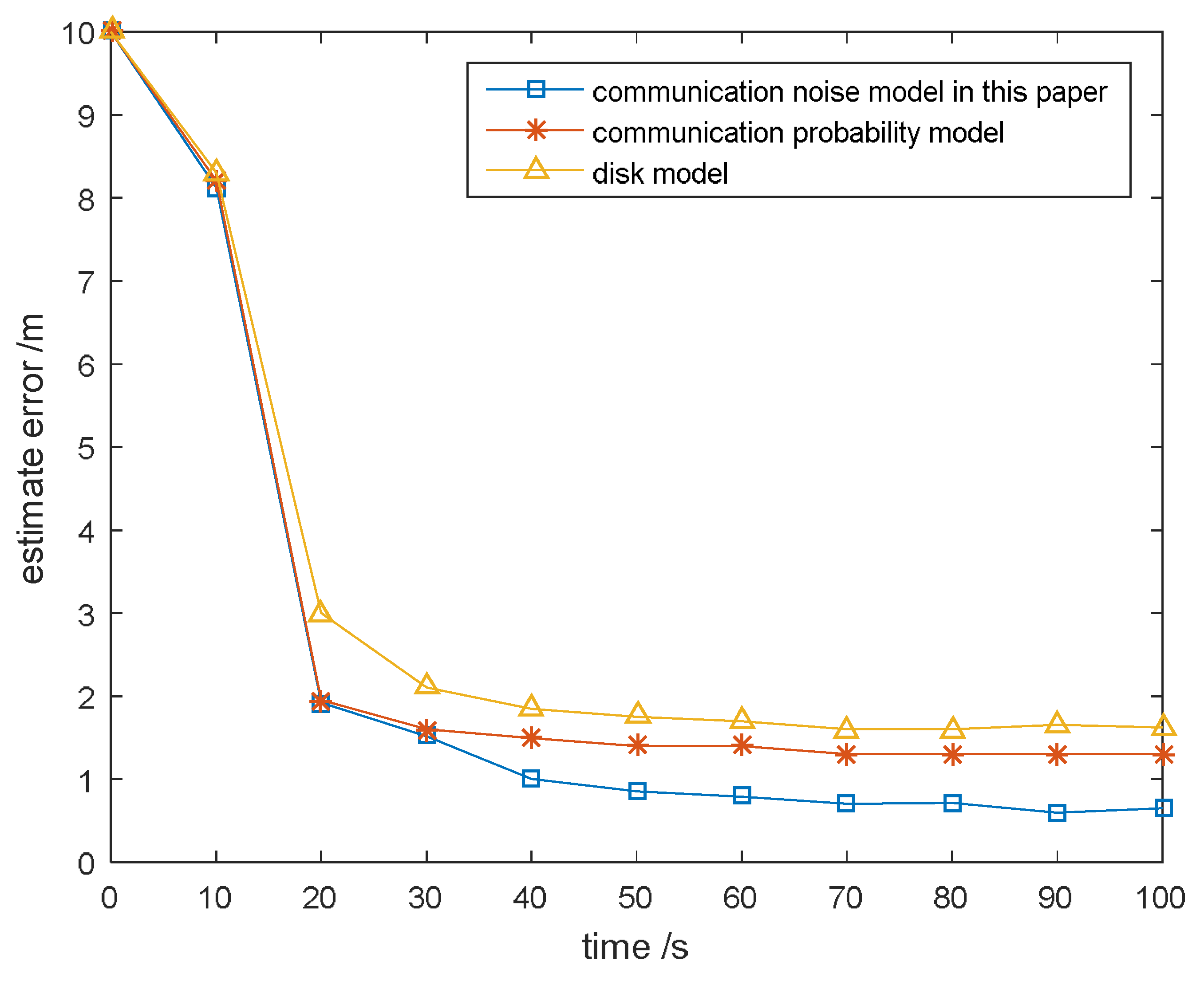
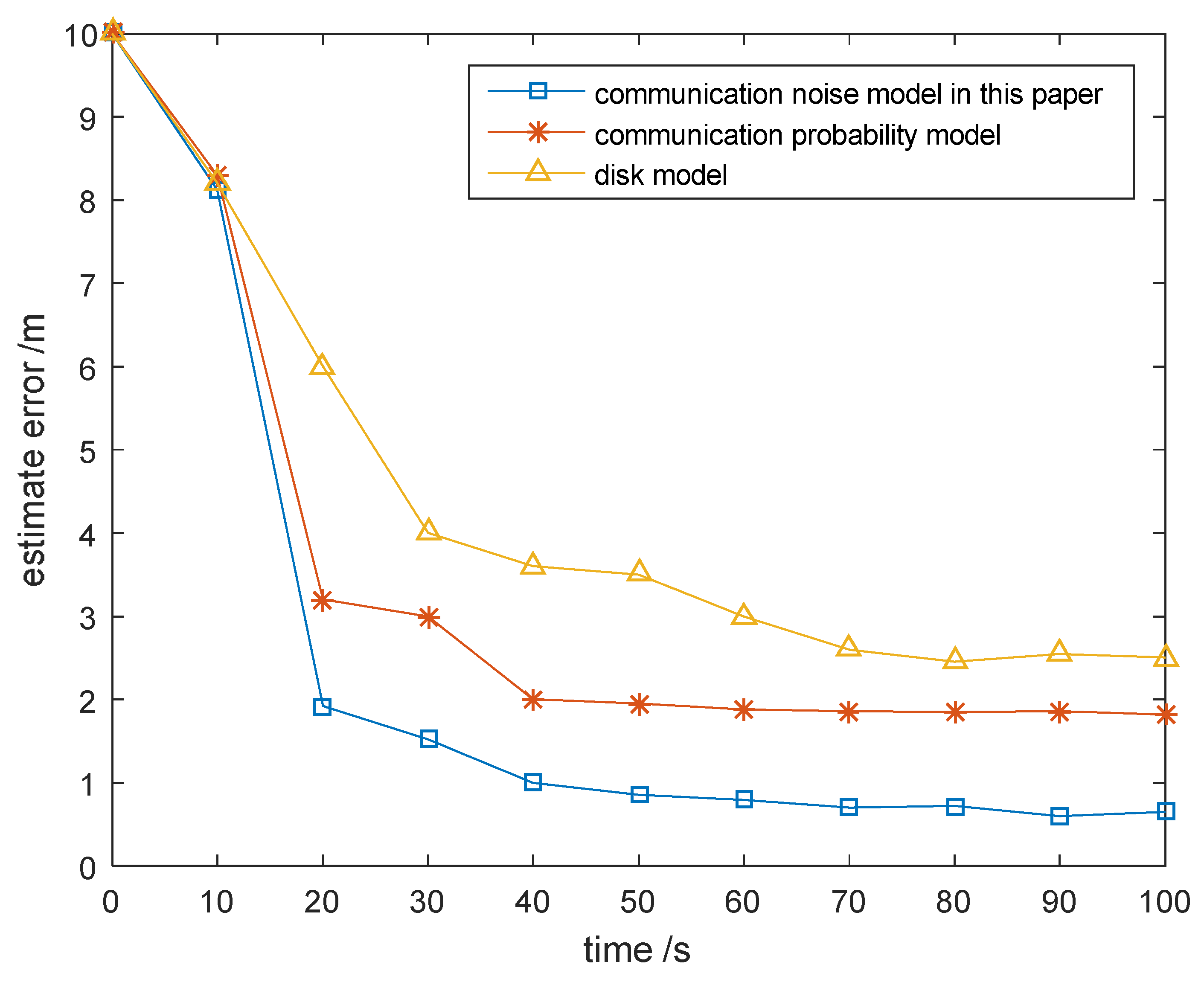
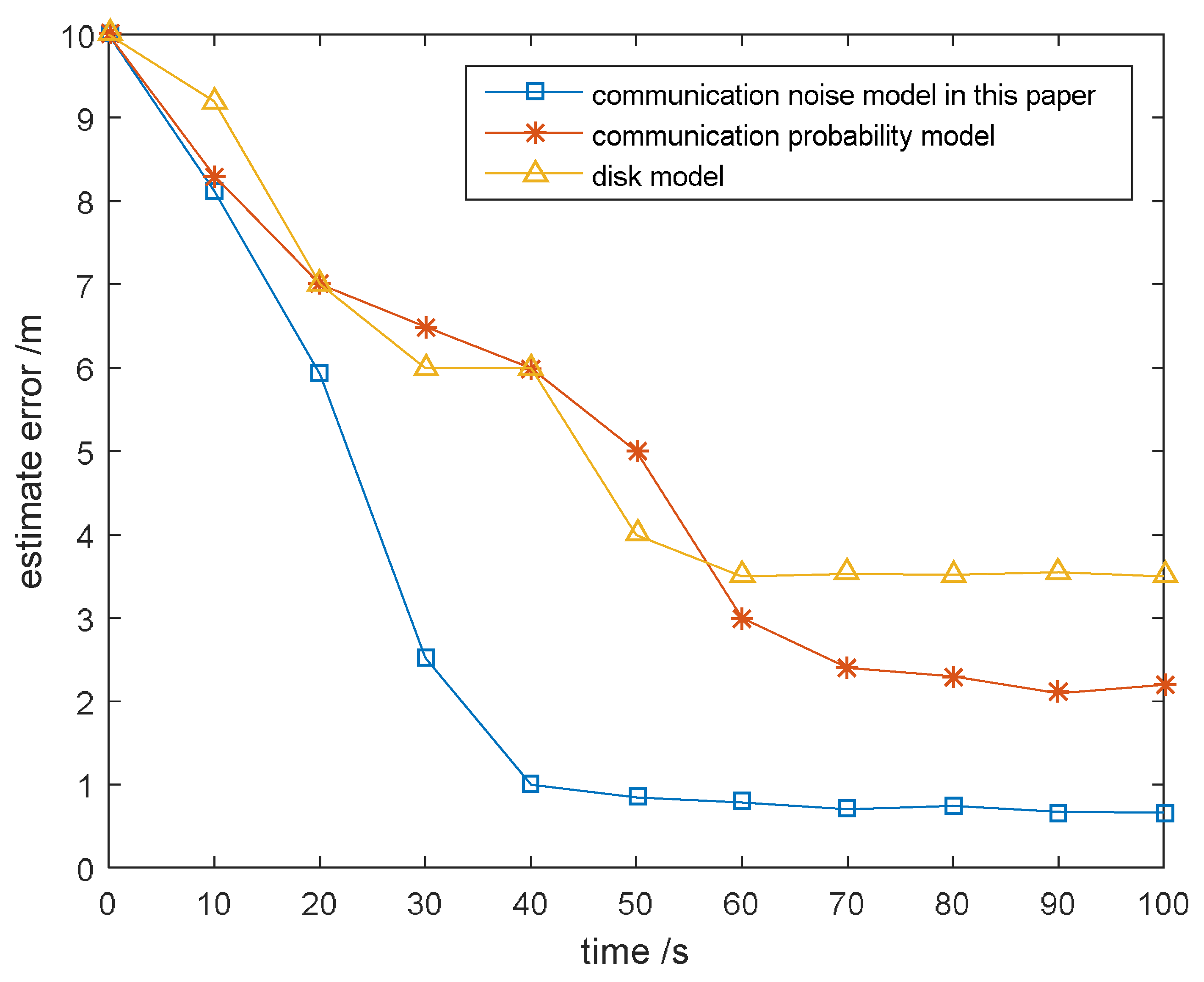
Figure 6, Figure 7 and Figure 8 show the performance of three different methods for estimating the target. Figure 6 shows the situation when the received signal power was only attenuated as a function of the distance between two nodes. Figure 7 shows the result in fading environment and Figure 8 shows the performance when there existed interference between UAVs.

In each condition of Figure 6, Figure 7 and Figure 8, we ran Monte-Carlo simulations 100 times for each model. Compared with the communication probability model, it turned out that our proposed method in this paper had a pretty good performance.

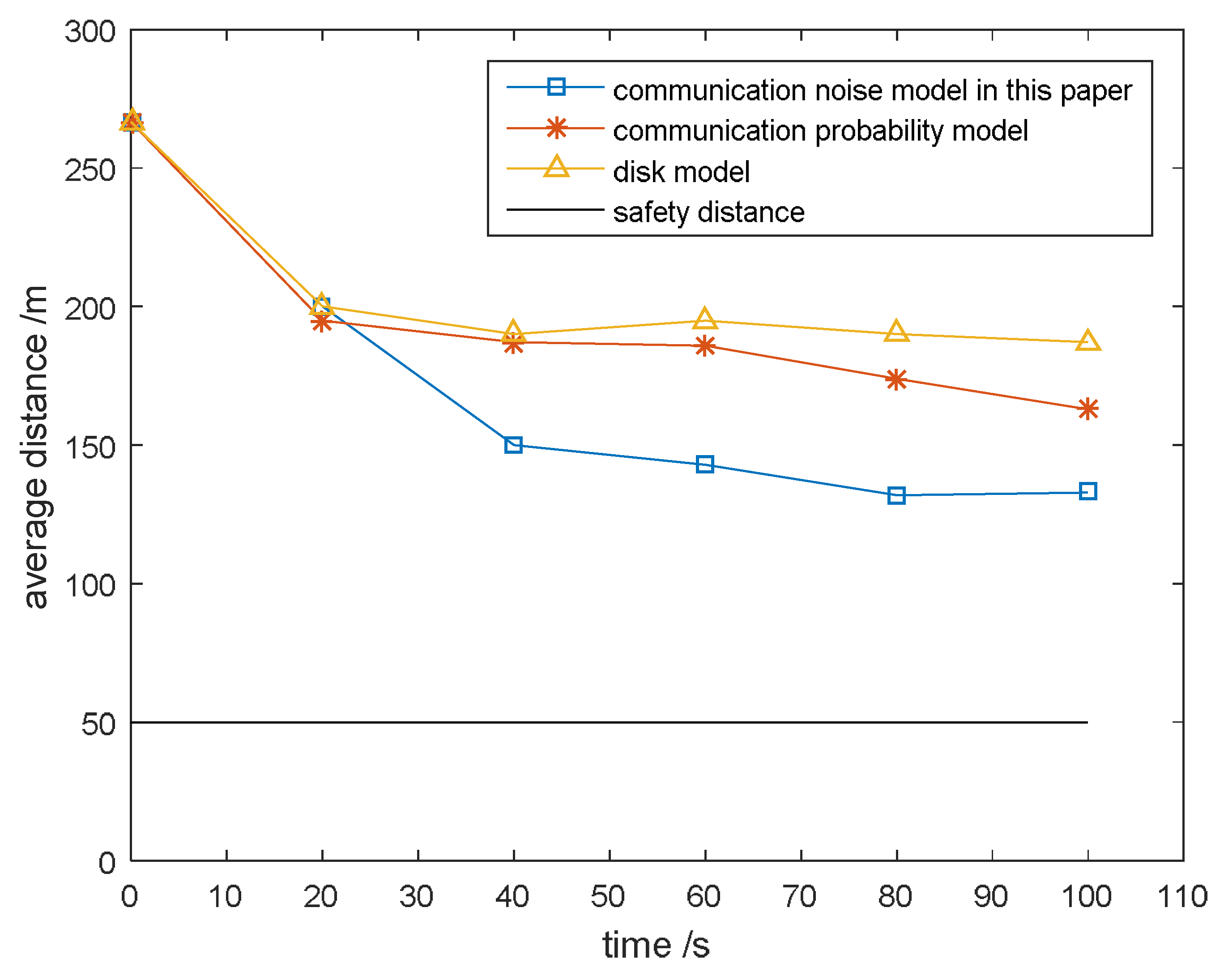
The results shown in Figure 9 are the average distance between UAVs with different methods. The safety distance was 50 m. We can see that the method in this paper had the shortest distance, which means the communication with our method was better than others.

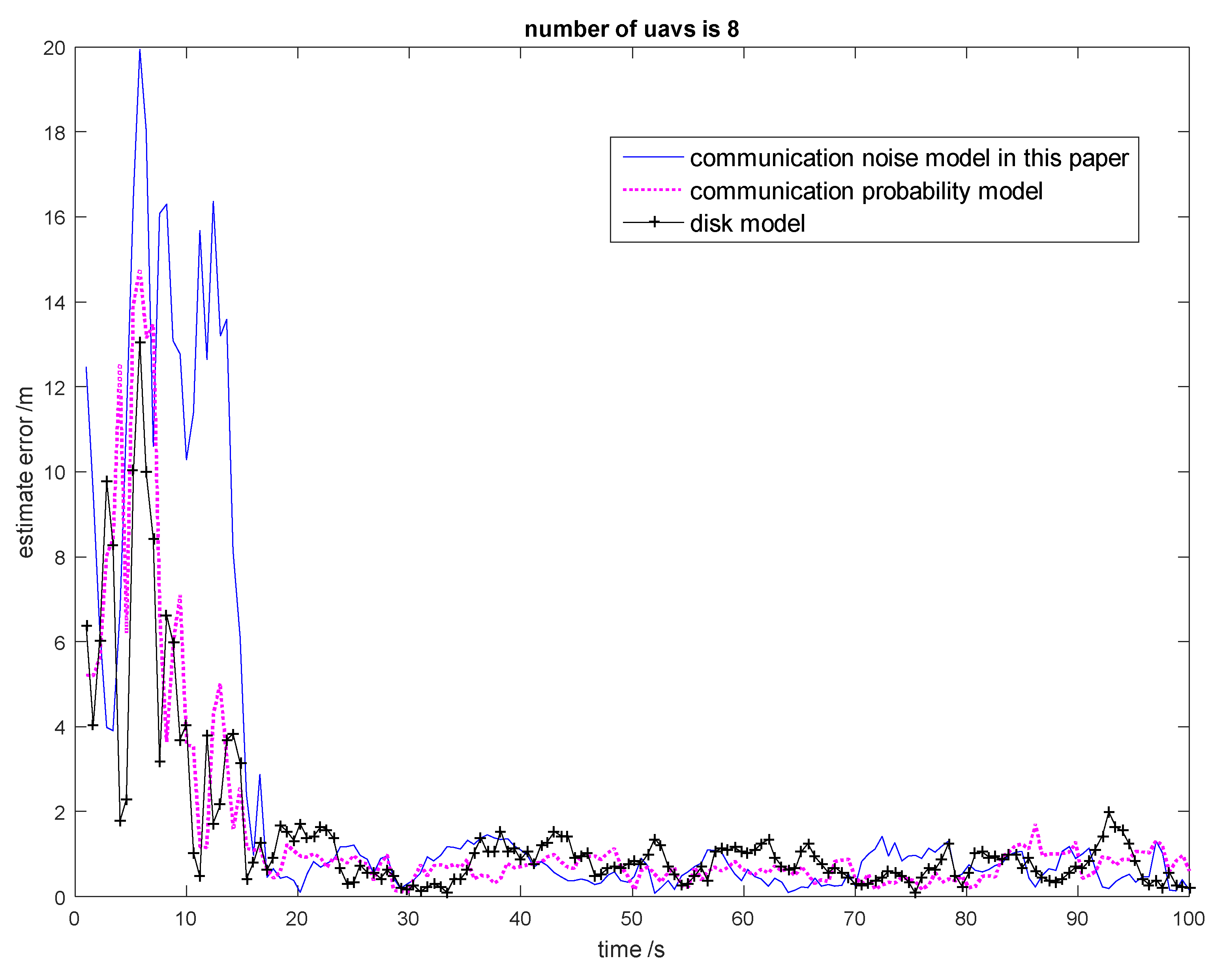
Figure 10 shows the effect of UAV numbers on estimate error. We can see that as the number of UAV increased, the average estimate error decreased. When the number of UAVs was larger than 6, we ran Monte-Carlo simulation 100 times and found that the estimated error was very small and close with different methods, which can be seen in Figure 11 (the number of UAVs was 8).

In Figure 11, we can see that at the beginning of the simulation, the estimation error of our method was higher than others. According to Equation (32), communication noise was treated as part of the observation noise. When the distance between UAVs was large, the communication channel quality was relatively low, so the communication noise was loud and caused a great estimate error. As the simulation continued, the error dropped quickly and stayed stable and small.

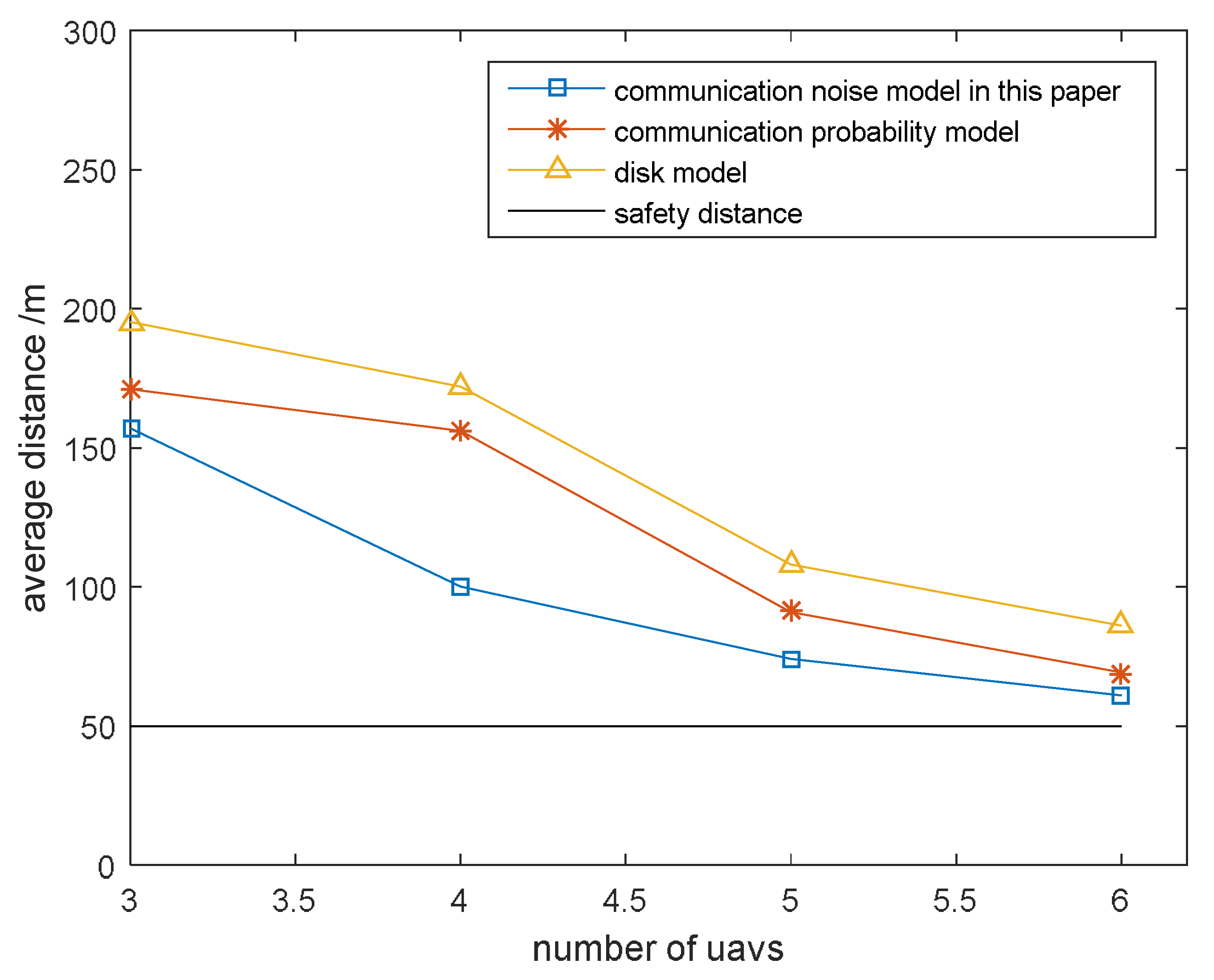
It can be seen in Figure 12 that when the number of UAVs increased, the distance between the UAVs decreased. This is because when different communication models were used, different observation configurations are obtained, which causes different average distances. When the distance between UAVs was small, there was low communication noise, which explained why these three methods had a very close estimate error in Figure 11 when the number of UAVs was very large.

6. Conclusions

A communication-aware cooperative target tracking algorithm was proposed, which is based on information consensus under multi-UAVs communication noise.

The communication between UAVs was modeled as a signal-to-interference-plus-noise ratio (SINR) model. When the receiver SNR of i-th UAV from j-th UAV was greater than a threshold, we assumed i-th UAV was j-th UAV’s neighbor. An UAV could communicate with its neighbors. Each UAV had a local filter to get an estimate and could receive its neighbors’ observation. Each UAV used the extended information filter to fusion its local observation and its’ neighbors’ observation to get a better estimate.

Each UAV calculated its own target tracking control inputs using receding horizon optimization method based on the consistency target state estimation.

The simulation results showed that the proposed communication model could make UAVs improve the accuracy of cooperative target tracking.

References

- Fu, X.W.; Gao, X.G. Effective Real-Time Unmanned Air Vehicle Path Planning in Presence of Threat Netting. J. Aerosp. Inf. Syst. 2014, 11, 170–177. [Google Scholar]
- Fu, X.W.; Bi, H.Y.; Gao, X.G. Multi-UAVs Cooperative Localization Algorithms with Communication Constraints. Math. Prob. Eng. 2017, 2017, 1943539. [Google Scholar] [CrossRef]
- Fu, X.W.; Feng, H.C.; Gao, X.G. UAV Mobile Ground Target Pursuit Algorithm. J. Intell. Robot. Syst. 2012, 68, 359–371. [Google Scholar] [CrossRef]
- Vercauteren, T.; Wang, X. Decentralized sigma-point information filters for target tracking in collaborative sensor networks. IEEE Trans. Signal Process. 2005, 53, 2997–3009. [Google Scholar] [CrossRef]
- Zhou, J.; Wang, Q. Convergence Speed in Distributed Average Consensus over Dynamically Switching Random Networks. Automatica 2009, 45, 1455–1461. [Google Scholar] [CrossRef]
- Liu, C.L.; Tian, Y.P. Survey on consensus problem of multi-agent systems with time delays. Control Decis. 2009, 24, 1601–1609. (In Chinese) [Google Scholar]
- Manolescu, D.A.; Meijer, E. Mobile Sensor Network. U.S. Patent 848,366,9B2, 9 July 2013. [Google Scholar]
- Li, Z.-G.; Zhou, X.-S. Computer Application Study. Sens. Netw. 2004, 21, 9–12. [Google Scholar]
- Stachura, M. Cooperative Target Localization with a Communication-Aware Unmanned Aircraft System. J. Guid. Control Dyn. 2011, 34, 1352–1362. [Google Scholar] [CrossRef]
- Mihaylova, L. Active Sensing for Robotics—A Survey. Proc. Numer. Methods Appl. 2002, 316–324. Available online: http://citeseer.ist.psu.edu/viewdoc/summary?doi=10.1.1.18.5320&rank=1&q=Active%20Sensing%20for%20Robotic-A%20Survey&osm=&ossid= (accessed on 20 March 2018).
- Mostofi, Y. Decentralized Communcation-Aware Motion Planning in Mobile Networks: An Information-Gain Approach. IEEE Trans. Autom. Control 2009, 56, 233–256. [Google Scholar]
- Ramachandra, K.V. Kalman Filter Techniques for Radar Tracking; Marcel Dekker: New York, NY, USA, 2000. [Google Scholar]
- Mozaffari, M.; Saad, W.; Bennis, M.; Debbah, M. Unmanned Aerial Vehicle with Underlaid Device-to-Device Communications: Performance and Tradeoffs. IEEE Trans. Wirel. Commun. 2016, 15, 3949–3963. [Google Scholar] [CrossRef]
- Zhang, S.; Zeng, Y.; Zhang, R. Cellular-enabled UAV communication: Trajectory optimization under connectivity constraint. In Proceedings of the IEEE International Conference on Communications (ICC), Kansas City, MO, USA, 20–24 May 2018. [Google Scholar]
- Xie, L.; Xu, J.; Zhang, R. Throughput maximization for UAV-enabled wireless powered communication networks. In Proceedings of the IEEE Vehicular Technology Conference (VTC), Porto, Portugal, 3–6 June 2018. [Google Scholar]
- Wu, Q.; Zeng, Y.; Zhang, R. Joint trajectory and communication design for UAV-enabled multiple access. In Proceedings of the IEEE Global Communications Conference (Globecom), Singapore, 4–8 December 2017. [Google Scholar]
- Mozaffari, M.; Saad, W.; Bennis, M.; Debbah, M. Wireless Communication using Unmanned Aerial Vehicles (UAVs): Optimal Transport Theory for Hover Time Optimization. IEEE Trans. Wirel. Commun. 2017, 16, 8052–8066. [Google Scholar] [CrossRef]
- Mozaffari, M.; Saad, W.; Bennis, M.; Debbah, M. Mobile Unmanned Aerial Vehicles (UAVs) for Energy-Efficient Internet of Things Communications. IEEE Trans. Wirel. Commun. 2017, 16, 7574–7589. [Google Scholar] [CrossRef]
- Lyu, J.; Zeng, Y.; Zhang, R. Spectrum sharing and cyclical multiple access in UAV-aided cellular offloading. In Proceedings of the IEEE Global Communications Conference (Globecom), Singapore, 4–8 December 2017. [Google Scholar]
- Zhu, M.; Liu, F.; Cai, Z.; Xu, M. Maintaining Connectivity of MANETs through Multiple Unmanned Aerial Vehicles. Math. Probl. Eng. 2015, 2015, 952069. [Google Scholar] [CrossRef]
- Jakes, W. Microwave Mobile Communications; IEEE: New York, NY, USA, 1974. [Google Scholar]
- Moore, T.; Stouch, D. A Generalized Extended Kalman Filter Implementation for the Robot Operation System; Springer: Berlin, Germany, 2016; Volume 302, pp. 335–348. [Google Scholar]
- Van der Merwe, R. The Unscented Particle Filter. In Proceedings of the International Conference on Neural Information Processing Systems, Denver, CO, USA, 28–30 November 2000; Volume 13, pp. 563–569. [Google Scholar]
- Ohtsuka, T. A Continuation/GMRES Method for Fast Compution of Nonliner Receding Horizon Control. Automatica 2004, 40, 563–574. [Google Scholar] [CrossRef]
- Goulart, P.J.; Kerrigan, E.C. A Method for Robust Receding Horizon Output Feedback Control of Constrained Systems. In Proceedings of the IEEE Conference on Decision & Control, San Diego, CA, USA, 13–15 December 2006; pp. 5471–5476. [Google Scholar]
- Liao, Y.; Li, H.; Bao, W. Indirect Radau Pseudospectral Method for the Receding Horizon Control Problem. Chin. J. Aeronaut. 2016, 29, 215–227. [Google Scholar] [CrossRef]
Figure 1.
Cooperative target tracking. UAV: Unmanned Aerial Vehicle.
Figure 2.
Information fusion structure.
Figure 3.
The observation configuration when N = 3.
Figure 4.
Target tracking trajectory with considering the communication noise between Unmanned Aerial Vehicles (UAVs).
Figure 5.
The average estimate error of the UAVs.
Figure 6.
The average estimate error compared with other methods in the presence of distance-dependent path loss.
Figure 7.
The average estimate error compared with other methods in fading environment.
Figure 8.
The average estimate error compared with other methods in presence of interference.
Figure 9.
The average distance between UAVs compared with other methods.
Figure 10.
The impact of number of UAVs on average estimate error.
Figure 11.
Estimate error with different methods (number of UAVs was 8).
Figure 12.
The impact of number of UAVs.