Article

Programmable Zoom Lens System with Two Spatial Light Modulators: Limits Imposed by the Spatial Resolution

1
Department of Physics, San Diego State University, San Diego, CA 92182-1233, USA
2
Departamento de Ciencia de Materiales, Óptica y Tecnología Electrónica, Universidad Miguel Hernández de Elche, 03202 Elche, Spain
*
Author to whom correspondence should be addressed.
Appl. Sci. 2018, 8(6), 1006; https://doi.org/10.3390/app8061006
Submission received: 10 May 2018 / Revised: 1 June 2018 / Accepted: 14 June 2018 / Published: 20 June 2018

Abstract

:

Featured Application

This proof-of-concept work might find applications as programmable zoom systems for imaging systems or holographic projection systems, when applied with newer high resolution SLMs.

Abstract

In this work we present an experimental proof of concept of a programmable optical zoom lens system with no moving parts that can form images with both positive and negative magnifications. Our system uses two programmable liquid crystal spatial light modulators to form the lenses composing the zoom system. The results included show that images can be formed with both positive and negative magnifications. Experimental results match the theory. We discuss the size limitations of this system caused by the limited spatial resolution and discuss how newer devices would shrink the size of the system.

1. Introduction

Optical zoom systems are basic components of all optical imaging systems. These zoom systems change the magnification of the image without altering the position of the object and image planes. They are usually composed of lens systems, in which a mechanical displacement of the lenses varies the effective magnification of the system, while keeping fixed object and image planes [1].
The design of zoom lenses without mechanical movements has been proposed since the early production of tunable lenses [2]. Programmable active lenses are currently available with different technologies, including liquid lenses [3], liquid-crystal lenses [4,5], or active polymer lenses [6]. Pancharatnam–Berry (PB) lenses are a new technology useful to overcome the slow response time of other technologies [7]. Therefore, zoom lenses with tunable adjustment and no moving elements have been reported [8,9,10,11].
Phase-only spatial light modulators (SLMs) are also very useful devices to display a lens function. They can display lenses where the focal length can be controlled directly by the geometry of the pattern addressed from a computer. They are diffractive lenses, and therefore they are affected by chromatic dispersion. They also require the use of polarized light. In addition, the pixelated structure of the SLMs impose limits on the shortest focal length that can be implemented. Nevertheless, SLMs allow a great flexibility to combine multiple lens functions [12], to multiplex the lens function with other holographic functions [13], or to correct aberrations [14]. These functions cannot be implemented with other kinds of tunable lenses.
Zoom lenses composed by SLMs have been reported previously [15]. In ref. [16], an anamorphic zoom lens system was demonstrated that used two SLMs. In Refs. [17,18], a holographic zoom lens projector using SLMs was also produced. However, SLMs present certain limitations and artifacts that make lenses displayed on them differ from the perfect idealized paraxial tunable lens. Nonlinear phase modulation, quantization of the phase levels, amplitude and/or polarization modulation coupled to phase modulation, fringing effects, phase fluctuation (flicker), or non-flatness panels that introduce aberrations, are some of the typical phenomena that one can find in these devices [13]. All these effects deteriorate the optical performance of lenses displayed onto SLM and must be considered and reduced, when possible.
In this work, we discuss the limits imposed by the rasterized structure of the SLM and give details for its experimental implementation in a simple zoom system composed of two lenses. We present configurations, which allow for different magnifications, and also to change the sign of the magnification to obtain both erect and inverted images. Because we employ SLMs with relatively large pixel sizes, we are forced to build a very large optical system, impractical for realistic applications. However, the results here presented constitute an experimental proof-of-concept that can be made useful and compact by using the newer SLM technology.

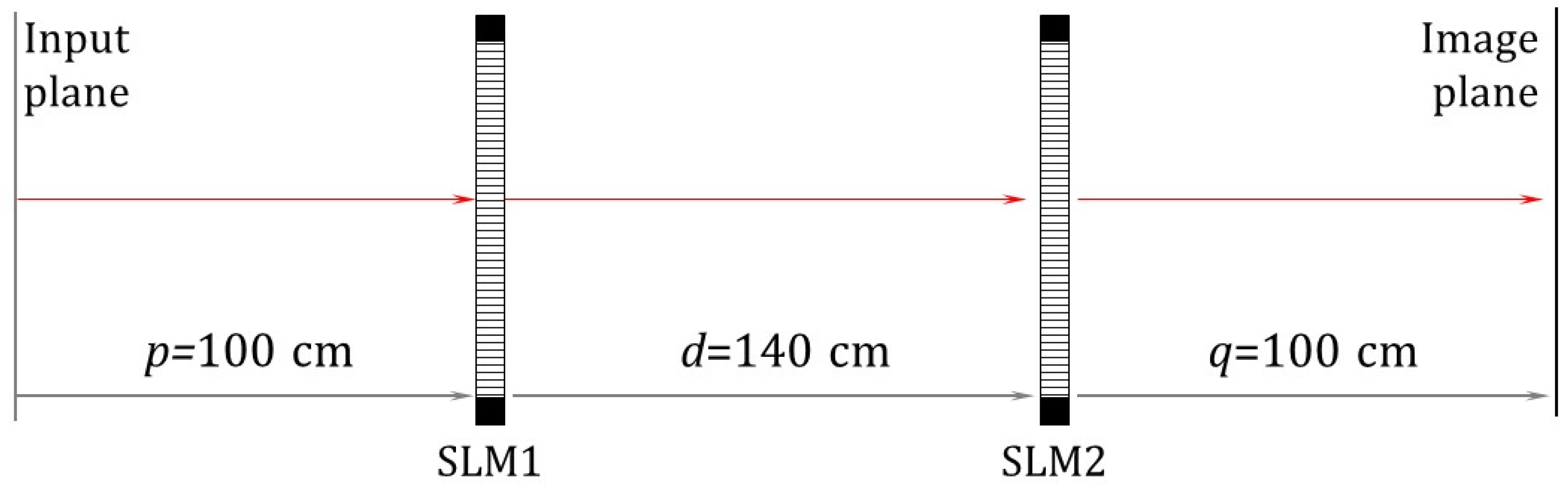
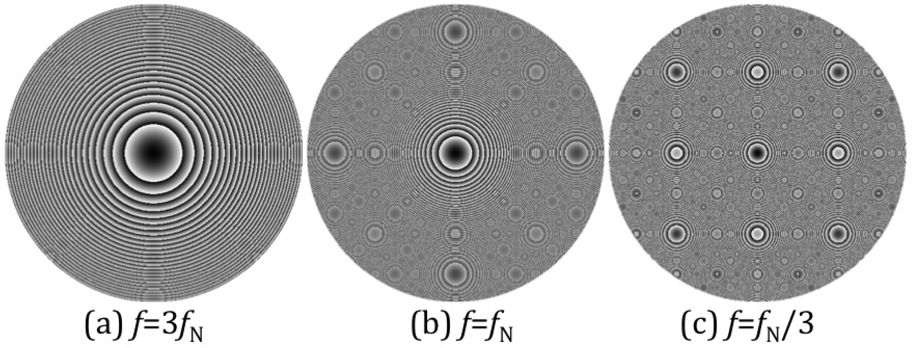
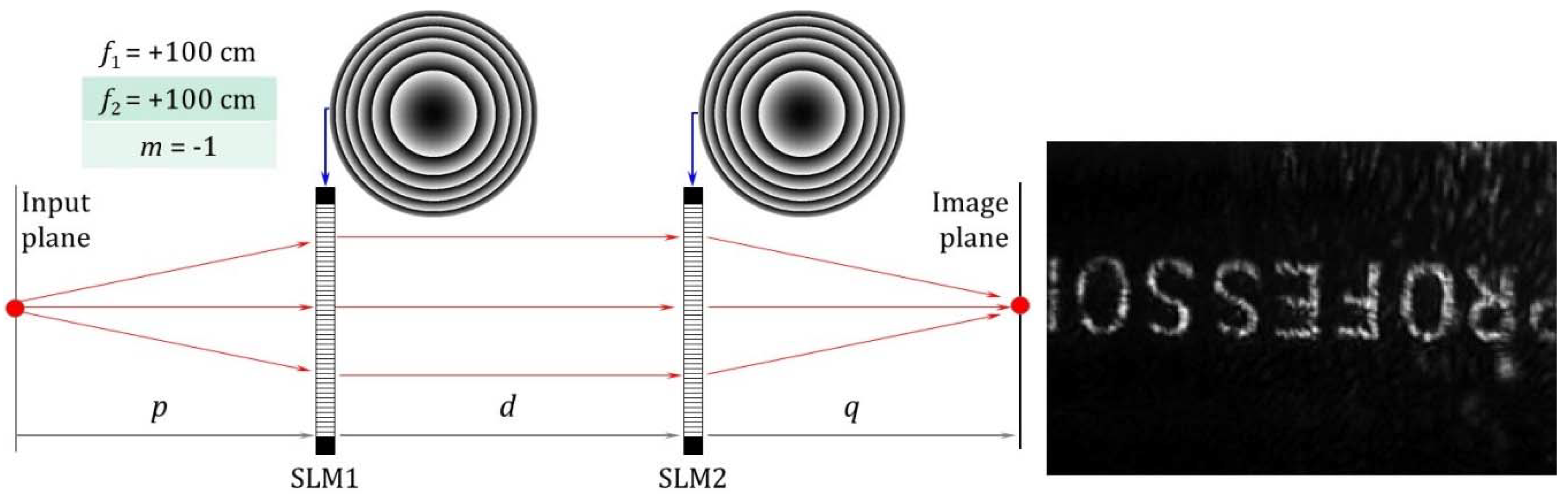
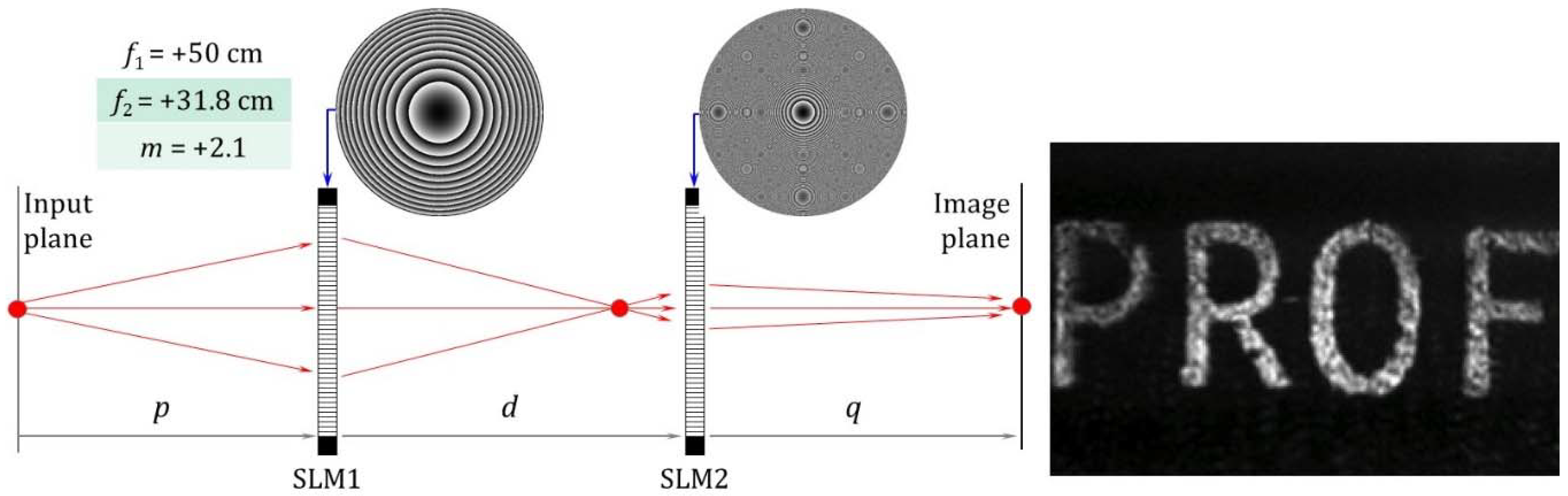
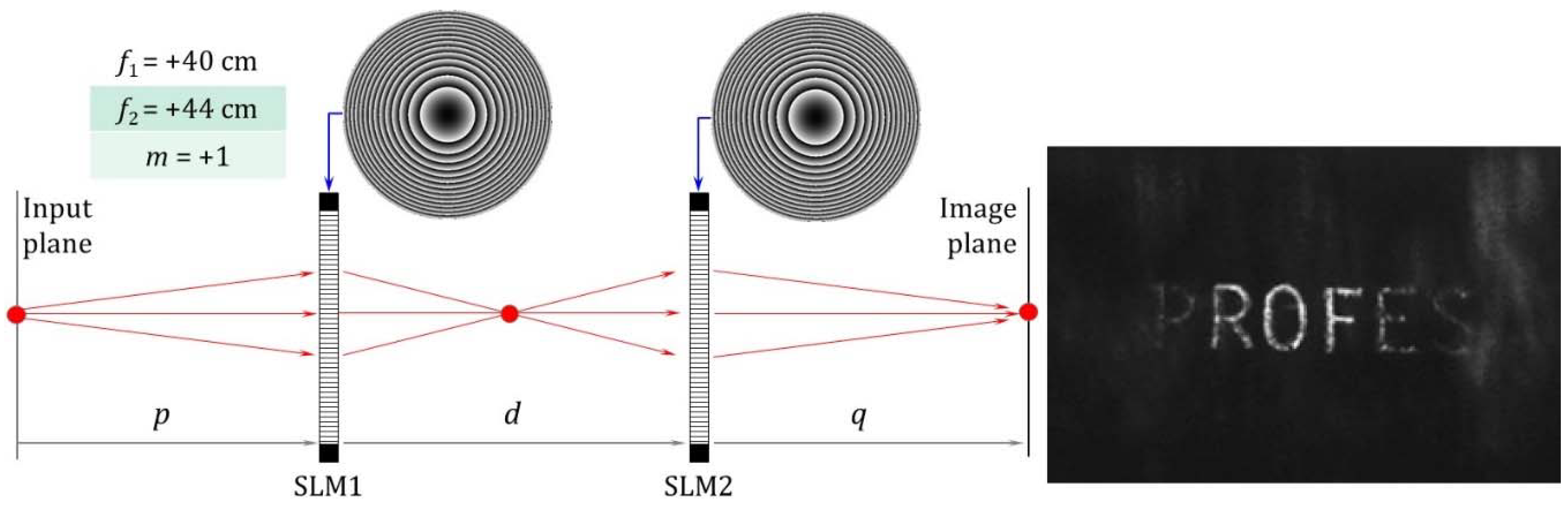
2. Geometry of the System

Figure 1 shows the configuration of our optical system. A programmable SLM is placed a distance p = 100 cm from an input object. The object (a slide transparency with the word “PROFESSOR”) is illuminated by a collimated beam from a helium-neon laser, with the λ = 633 nm wavelength. A second SLM is placed a distance d = 140 cm from the first. Finally, the camera is located a distance also approximately q = 100 cm from the second SLM. The output patterns were recorded with a CCD camera, model XC-37 (Sony, USA), having 491 × 384 pixels on a 8.86 × 6.60 mm2 sensor.
Note that zoom lenses used in photography are designed to image distant objects, so p is a very large distance. Tunable zoom lenses have also been demonstrated for holographic projection systems [17,18]. There, the p is a short distance, while q should be larger. Here we selected an intermediate approach where the object and image are located at finite close distances.
Using a standard ray matrix approach [19], this system can be represented by the product of three translation matrices and the two lens matrices as in Equation (1). The product of these matrices is given by the final ABCD matrix:
| r 2 r 2 | = | 1 q 0 1 | × | 1 0 1 / f 2 1 | × | 1 d 0 1 | × | 1 0 1 / f 1 1 | × | 1 p 0 1 | × | r 1 r 1 | = | A B C D | × | r 1 r 1 |
r i and r i (i = 1, 2) denote the ray height and angle coordinates.
The calculation of the ABCD matrix in Equation (1) leads to the following result:
| r 2 r 2 | = | 1 d f 1 q F p ( 1 d f 1 q F ) + d + q ( 1 d f 2 ) 1 F p F + 1 d f 2 | × | r 1 r 1 |
where F denotes the focal length of the composed system, given by:
1 F = 1 f 1 + 1 f 2 d f 1 f 2
The imaging requirement is met by forcing the matrix element B = 0. This condition leads to the following relation
f 2 = f 1 q ( d + p ) p d q f 1 ( p + d + q ) p ( d + q ) = f 1 q ( D q ) p d q f 1 D p ( D p )
where D = p + d + q is the total distance of the system, which we want to keep constant, so the system has no moving elements.
The magnification is given by the matrix element A in Equation (2), i.e.,
m = 1 d + q f 1 q f 2 q d f 1 f 2
The system is limited by the geometry of the SLMs. In this work, the first lens is encoded onto a CRL model XGA-3 transmissive twisted nematic SLM operating in a phase-only mode by means of the rotated eigen-polarization state technique [20]. This device has 1024 × 768 pixels with a pixel spacing of 18 microns. The second lens is formed on a Hamamatsu model X10468-01 reflective parallel-aligned SLM, also operating in a phase-only mode. This device has 800 × 600 pixels with a pixel spacing of 20 microns. Because this second SLM is a reflective liquid-crystal on silicon (LCoS) display, we include a beam splitter in the system to allow a reflective geometry in the second part of the system in Figure 1. Both displays use eight bits for codification of phase levels, i.e., they have N = 256 quantization levels. The first order diffraction efficiency caused by the quantization of phase levels is given by ηQ = [sin(π/N)/(π/N)]2 which for N = 256 levels results in a value of exceeding 99% [21]. Thus, quantization is not an issue for this system. Both SLMs have been tested and produce a phase-only response versus addressed gray level, with no cross-modulation effects. In addition, the phase modulation versus addressed gray level is linearized.
On the contrary, the limited spatial resolution imposes drastic losses and limits. Although both devices have similar pixel pitch, the LCoS technology presents a much higher fill factor (FF). The fill factor is defined as FF = (w/Δ)2, where w stands for the pixel width and Δ stands for the pixel spacing [22]. The CRL display has a fill factor of approximately only FFCRL ≈ 35%. In contrast, the Hamamatsu LCoS display presents a much higher value of approximately FFHAM ≈ 98%. This difference makes a major impact between the two devices. First, the fraction of the incident intensity that is transmitted is given directly by the FF. Secondly, the SLM rasterized structure created a 2D grid of diffraction orders. The central principal zero order has the highest intensity, which is roughly proportional to FF2 [22]. Since we are using the zero diffracted order in the zoom lens system, the total intensity transmission is reduced by this effect to a factor of ηFF = (FFCRL × FFHAM)2 ≈ 12%.
But, even more relevant for the application to the zoom lens system is the limitation imposed by the limited spatial resolution on the minimum focal length that the SLMs can encode. We have previously discussed [13] the limits imposed by the spatial resolution of the SLM when we implement a lens function having a quadratic phase dependence as:
Z * ( r , f ) = exp ( i π r 2 λ f )
where f denotes the focal length of the lens, λ is the wavelength and r denotes the radial coordinate at the SLM plane. Next, we summarize the main effect, for its implication in the zoom lens system.
We assume that the SLM has an array of N × N pixels where each pixel has a finite size given by Δ . As the focal length f of the encoded lens decreases, the spacing between the phase at the edges of the device can become smaller than the Nyquist limit of 2 pixels causing aliasing effects. These considerations lead to the Nyquist focal length (fN) for a lens encoded onto the SLM as given by [12]:
f N = N Δ 2 λ
Lens functions as in Equation (6) with focal lengths shorter (in absolute value) than the Nyquist focal length | f | f N are affected by aliasing and will not be well reproduced.
Figure 2 shows three diffractive lenses where the focal lengths are greater and smaller than the Nyquist limit. If the focal length is clearly greater than f N , the lens function is encoded perfectly. However, for shorter focal lengths the effective central area of the lens decreases and the lens begins to act as a low pass spatial filter. In addition, the strengths of the replica focal lengths caused by the aliasing increase.
For our SLMs, the effective Nyquist focal lengths are about 38 cm, considering the smaller dimensions. These considerations have important consequences for our optical system because the SLMs have difficulty encoding focal lengths smaller than this value. This limit requires the large values for the distances in our experimental system in Figure 1. These large dimensions of the zoom lens system make it impractical for real applications. However, we show results as discussed next that demonstrate the proof-of-concept and illustrate the potential usefulness of newer high resolution SLMs to build programmable zoom lens systems
Although the proper characterization of a zoom lens system requires the evaluation of parameters like resolution, field of view, modulation transfer function or contrast, we concentrate in these proof-of-concept results only in the different magnifications that the system can produce including a change of sign.

3. Experimental Imaging Results without Moving Elements

As stated earlier, the object is an opaque slide with the transparent word “PROFESSOR” having a size of roughly 9 × 1 mm. Figure 3 shows the image when the camera is placed directly against the slide, so the reader can compare the object size with the images formed for different configurations of the zoom system. Note that the image is not perfectly in focus due to the small propagation distance between the slide and the camera detector.

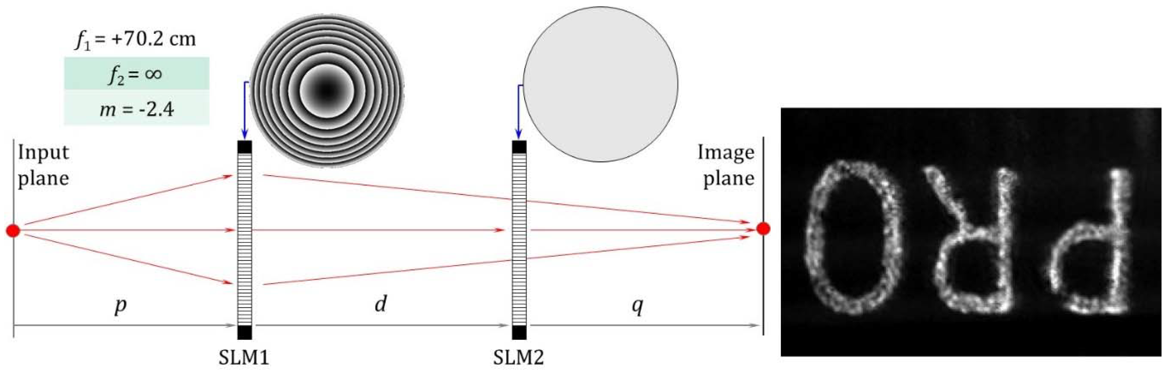
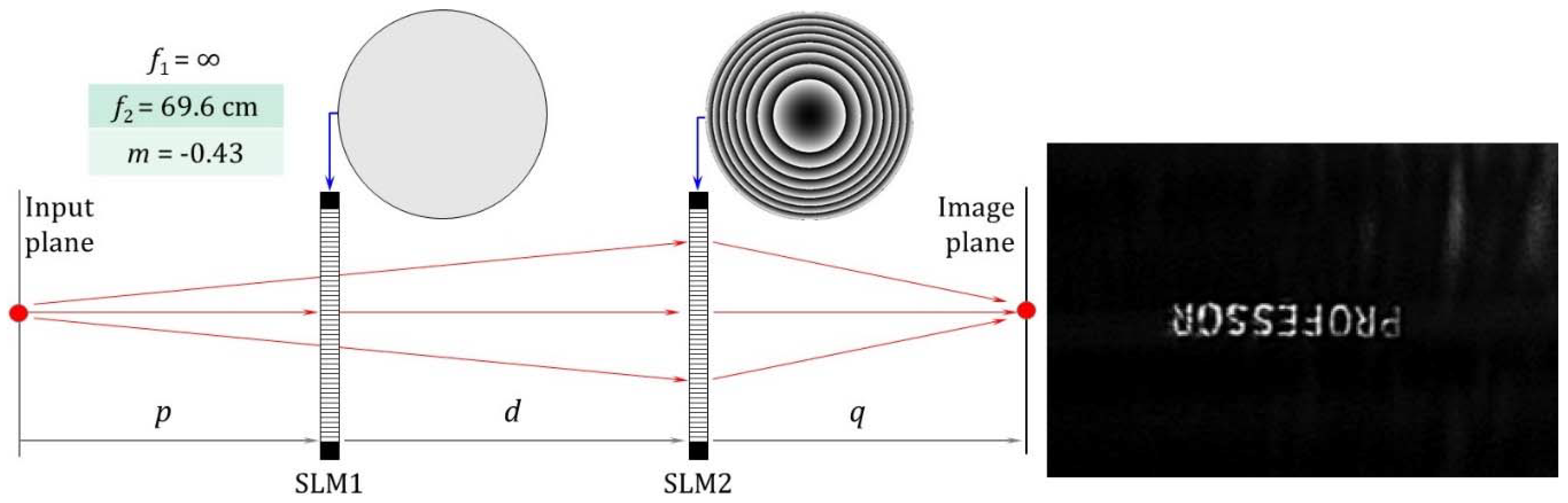
3.1. Negative Magnifications

We first examine cases where we obtain inverted images. Figure 4 presents the system configuration and the output image when the first SLM is encoded with a focal length of f 1 = 70.2 cm and the second SLM is turned off. Therefore, we have a single lens imaging system, where the object distance is p, and the image distance is d + q. The output is inverted with a magnification of about m = 2.3 in excellent agreement with the theoretical magnification obtained using Equation (5). The size of the image is larger than the detector. As we moved the position of the input slide, different areas of the letter were seen. We note that, in doing these experiments, we simply varied the focal length encoded onto the device until the image was focused. This procedure accounts for small deviations of the distances p, d and q.
Figure 5 shows the zoom system configuration and the output image when the first SLM is turned off and the second SLM is encoded with a focal length of f 2 = 69.6 cm. Again, we have a single lens imaging system, where now the image distance q is smaller than the object distance p + d. The output is inverted with a magnification of about m = −0.43 in excellent agreement with the theoretical magnification obtained by using Equation (5). The size of the image is smaller than the detector.
Finally, Figure 6 shows the output image when both devices are encoded with focal lengths of f 1 = f 2 = 100 cm. Now the focal length of the composite lens system is approximately F = 167 cm, and the object is inverted with a magnification of m = −1 in excellent agreement with theory. Note that this configuration places the input object plane in the front focal plane of the first lens and the final output image plane in the back focal plane of the second lens.
Note that in these three cases shown here, the encoded lenses have focal lengths larger than the Nyquist limit of 38 cm. Therefore, the displayed lenses are well reproduced and the final image is well focused in all cases. There is, however, some low pass filtering caused by the limited size of the SLMs compared to the long distances required in the system.

3.2. Positive Magnifications

In this section, we examine positive magnifications where the image has the same orientation as the object. These results have not been previously presented, to our knowledge. In each case, the first lens forms a real image between the two lenses that is inverted and serves as a real object for the second lens. This second lens then forms the erect image.
Figure 7 shows the case where the first SLM is encoded with a focal length of f 1 = 50 cm while the second SLM is encoded with a focal length of f 2 = 31.8 cm. Note that this second focal length is below the Nyquist limit. The composed system has a negative focal length of about F = −27 cm. We now obtain an erect image with a magnification of m = +2 in excellent agreement with the theoretical value. The size of the image is larger than the detector.
Figure 8 shows the case where the first SLM is encoded with a focal length of f 1 = 31.8 cm while the second SLM is encoded with a focal length of f 2 = 50 cm. Now the first lens has a focal length shorter than the Nyquist limit. The composed system again has a negative focal length of about F = −27 cm. Again we obtain an erect image, but with a smaller magnification of m = +0.5 in excellent agreement with theory. We cannot capture the entire image, unlike the case in Figure 5. In this case because of the short focal length of the first lens, the rays forming the external points of the intermediate image do not enter the second lens. This effect is similar to that shown in the holographic zoom system in ref. [17]. As we moved the object, other parts of the image would come into view. This effect is also present in Figure 7, but is not as visible because of the large magnification such that the image is larger than the area of the camera.
Finally, Figure 9 shows the case where the first SLM is encoded with a focal length of f 1 = 40 cm while the second SLM is encoded with a focal length of f 2 = 44 cm. The composed system again has a negative focal length of about F = −31 cm. Again we obtain an erect image, but with a magnification of m = +1.0 in excellent agreement with theory. Again, we cannot capture the entire image because of the short focal lengths required.

4. Conclusions

In conclusion, we demonstrate a programmable zoom lens system where the magnification and sense of the image can be controlled without moving any parts. We use two programmable SLMs onto which we can encode the required focal length lenses to achieve these results. We note that the physical size of this system is extremely large primarily because of the small sizes of the lenses (diameters of 14 mm and 12 mm respectively) and the Nyquist limits on the focal lengths that we can encode onto our SLMs.
However, there are new high resolution 4KUHD(Ultra-High Definition) SLM models having a pixel size as small as 3.74 microns in an array of 3840 × 2160 pixels (data from the Exulus-4K1 model [23] offered by Thorlabs), or 4160 × 2464 (data from the the GAEA-2 model [24], offered by Holoeye). The pixel spacing of these SLMs lead to a Nyquist focal length limit of about 50 mm. These devices would allow a much more compact zoom lens system.
Another strategy for reducing the size of the system is to combine the lenses displayed on the SLMs with other glass lenses that add a constant optical power. However, for simplicity, here we analyze the system where all the optical power is encoded only on the SLMs.
Nevertheless, we obtain excellent results and show a proof-of-concept of a zoom system without moving elements based on SLMs, and showing negative magnifications ranging from −2 to −1/2 and negative magnifications from +2 to +1/2. The use of SLMs to produce the zoom system can be very promising since other functionalities of SLMs like wavefront aberration correction, optical processing functions, or polarization control can be incorporated into the system.

Author Contributions

Conceptualization, J.A.D. and I.M.; Methodology, J.A.D., I.M. and D.M.C.; Software, D.M.C.; Validation, J.A.D., T.I.H., and J.P.S.; All authors; Writing-Review & Editing, J.A.D.; Supervision, J.A.D.

Funding

The participation of I.M. in this investigation was funded by Ministerio de Economía y Competitividad from Spain and FEDER Funds (ref. FIS2015-66328-C3-3-R) and from Conselleria d’Educació, Investigació, Cultura i Esport, Generalitat Valenciana (ref. PROMETEO-2017-154).

Conflicts of Interest

The authors declare no conflict of interest.

References

  1. Youngworth, R.N.; Betensky, E.I. Fundamental considerations for zoom lens design. Proc. SPIE 2012, 8488, 848806. [Google Scholar]
  2. Tam, E.C. Smart electro-optical zoom lens. Opt. Lett. 1992, 17, 369–371. [Google Scholar] [CrossRef] [PubMed]
  3. Kuiper, S.; Hendriks, B.H.W. Variable-focus liquid lens for miniature cameras. Appl. Phys. Lett. 2004, 85, 1128–1130. [Google Scholar] [CrossRef]
  4. Ren, H.; Fox, D.W.; Wu, B.; Wu, S.T. Liquid crystal lens with large focal length tunability and low operating voltage. Opt. Express 2007, 15, 11328–11335. [Google Scholar] [CrossRef] [PubMed]
  5. Jamali, A.; Bryant, D.; Zhang, Y.; Grunnet-Jepsen, A.; Bhowmik, A.; Bos, P. Design of a large aperture tunable refractive Fresnel liquid crystal lens. Appl. Opt. 2018, 57, B10–B19. [Google Scholar] [CrossRef] [PubMed]
  6. Yun, S.; Park, S.; Nam, S.; Park, B.; Park, S.K.; Mun, S.; Lim, J.M.; Kyung, K.-U. An electro-active polymer based lens module for dynamically varying focal system. Appl. Phys. Lett. 2016, 109, 141908. [Google Scholar] [CrossRef]
  7. Lee, Y.-H.; Tan, G.; Zhan, T.; Weng, Y.; Liu, G.; Gou, F.; Peng, F.; Tabiryan, N.V.; Gauza, S.; Wu, S.-T. Recent progress in Pancharatnam–Berry phase optical elements and the applications for virtual/augmented realities. Opt. Data Process. Storage 2017, 3, 79–88. [Google Scholar] [CrossRef] [Green Version]
  8. Santiago, F.; Bagwell, B.E.; Pinon, V.; Krishna, S. Adaptive polymer lens for rapid zoom shortwave infrared imaging applications. Opt. Eng. 2014, 53, 125101. [Google Scholar] [CrossRef]
  9. Li, H.; Cheng, X.; Hao, Q. An electrically tunable zoom system using liquid lenses. Sensors 2016, 16, 45. [Google Scholar] [CrossRef] [PubMed]
  10. Li, L.; Yuan, R.-Y.; Wang, J.-H.; Wang, Q.-H. Electrically optofluidic zoom system with a large zoom range and high-resolution image. Opt. Express 2017, 25, 22280–22297. [Google Scholar] [CrossRef] [PubMed]
  11. Kopp, D.; Brender, T.; Zappe, H. All-liquid dual-lens optofluidic zoom system. Appl. Opt. 2017, 56, 3758–3763. [Google Scholar] [CrossRef] [PubMed]
  12. Cottrell, D.M.; Davis, J.A.; Hedman, T.R.; Lilly, R.A. Multiple imaging phase-encoded optical elements written as programmable spatial light modulators. Appl. Opt. 1990, 29, 2505–2509. [Google Scholar] [CrossRef] [PubMed]
  13. Haist, T.; Osten, W. Holography using pixelated spatial light modulators—Part 1: Theory and basic considerations. J. Micro/Nanolithogr. MEMS MOEMS 2015, 14, 041310. [Google Scholar] [CrossRef]
  14. Neil, M.A.A.; Booth, M.J.; Wilson, T. Closed-loop aberration correction by use of a modal Zernike wave-front sensor. Opt. Lett. 2000, 25, 1083–1085. [Google Scholar] [CrossRef] [PubMed]
  15. Wick, D.V.; Martinez, T. Adaptive optical zoom. Opt. Eng. 2004, 43, 8–9. [Google Scholar]
  16. Iemmi, C.; Campos, J. Anamorphic zoom system based on liquid crystal displays. J. Eur. Opt. Soc. Rapid Pub. 2009, 4, 09029. [Google Scholar] [CrossRef]
  17. Lin, H.-C.; Collings, N.; Chen, M.-S.; Lin, Y.-H. A holographic projection system with an electrically tuning and continuously adjustable optical zoom. Opt. Express 2012, 20, 27222–27229. [Google Scholar] [CrossRef] [PubMed]
  18. Chen, M.-S.; Collings, N.; Lin, H.-C.; Lin, Y.-H. A holographic projection system with an electrically adjustable optical zoom and a fixed location of zeroth-order diffraction. J. Disp. Technol. 2014, 10, 450–455. [Google Scholar] [CrossRef]
  19. Davis, J.A.; Lilly, R.A. Ray-matrix approach for diffractive optics. Appl. Opt. 1993, 32, 155–158. [Google Scholar] [CrossRef] [PubMed]
  20. Davis, J.A.; Moreno, I.; Tsai, P. Polarization eigenstates for twisted-nematic liquid crystal displays. Appl. Opt. 1998, 37, 937–945. [Google Scholar] [CrossRef] [PubMed]
  21. Moreno, I.; Iemmi, C.; Márquez, A.; Campos, J.; Yzuel, M.J. Modulation light efficiency of diffractive lenses displayed onto a restricted phase-mostly modulation display. Appl. Opt. 2004, 43, 6278–6284. [Google Scholar] [CrossRef] [PubMed]
  22. Davis, J.A.; Chambers, J.B.; Slovick, B.A.; Moreno, I. Wavelength dependent diffraction patterns from a liquid crystal display. Appl. Opt. 2008, 47, 4375–4380. [Google Scholar] [CrossRef] [PubMed]
  23. Exulus Spatial Light Modulator. Available online: https://www.thorlabs.com/newgrouppage9.cfm?objectgroup_id=10378 (accessed on 19 June 2018).
  24. GAEA-2 Megapixel Phase Only Spatial Light Modulator (Refective). Available online: https://holoeye.com/spatial-light-modulators/gaea-4k-phase-only-spatial-light-modulator/ (accessed on 19 June 2018).
Figure 1. Schematic of the zoom lens optical system.
Applsci 08 01006 g001
Figure 2. Phase patterns for diffractive lenses having focal lengths of (a) 3fN, (b) fN and (c) fN/3.
Applsci 08 01006 g002
Figure 3. Input object captured by camera. Here the slide with the word “PROFESSOR” is placed directly to the detector. The size of the object slightly exceeds the size of the detector.
Applsci 08 01006 g003
Figure 4. Zoom system configuration with f1 = 70.2 cm and f2 = ∞ and experimental image with magnification of m = −2.4.
Applsci 08 01006 g004
Figure 5. Zoom system configuration with f1 = ∞ and f2 = +69.6 cm and experimental image with magnification of m = −0.4.
Applsci 08 01006 g005
Figure 6. Zoom system configuration with f1 = +100 cm and f2 = +100 cm and experimental image with magnification of m = −1.
Applsci 08 01006 g006
Figure 7. Zoom system configuration with f1 = +50 cm and f2 = +31.8 cm and experimental image with magnification of m = +2.
Applsci 08 01006 g007
Figure 8. Zoom system configuration with f1 = +31.8 cm and f2 = +50 cm and experimental image with magnification of m = +0.5.
Applsci 08 01006 g008
Figure 9. Zoom system configuration with f1 = +40 cm and f2 = +44 cm and experimental image with magnification of m = +1.
Applsci 08 01006 g009

