Prediction of HIFU Propagation in a Dispersive Medium via Khokhlov–Zabolotskaya–Kuznetsov Model Combined with a Fractional Order Derivative

Abstract

High intensity focused ultrasound (HIFU) has been proven to be promising in non-invasive therapies, in which precise prediction of the focused ultrasound field is crucial for its accurate and safe application. Although the Khokhlov–Zabolotskaya–Kuznetsov (KZK) equation has been widely used in the calculation of the nonlinear acoustic field of HIFU, some deviations still exist when it comes to dispersive medium. This problem also exists as an obstacle to the Westervelt model and the Spherical Beam Equation. Considering that the KZK equation is the most prevalent model in HIFU applications due to its accurate and simple simulation algorithms, there is an urgent need to improve its performance in dispersive medium. In this work, a modified KZK (mKZK) equation derived from a fractional order derivative is proposed to calculate the nonlinear acoustic field in a dispersive medium. By correcting the power index in the attenuation term, this model is capable of providing improved prediction accuracy, especially in the axial position of the focal area. Simulation results using the obtained model were further compared with the experimental results from a gel phantom. Good agreements were found, indicating the applicability of the proposed model. The findings of this work will be helpful in making more accurate treatment plans for HIFU therapies, as well as facilitating the application of ultrasound in acoustic hyperthermia therapy.

1. Introduction

Although pioneering clinical studies of focused ultrasound were carried out as early as the 1940s [1,2], it did not attract intensive research interest until the end of the 20th century and the beginning of 21st century, during which several theoretical models were developed, improved and then broadly accepted [3,4,5,6,7,8,9]. In the past decades, high intensity focused ultrasound (HIFU) has played an increasingly significant role in the study of non-invasive therapies by demonstrating unique advantages in safety, effectiveness and high efficiency [10,11,12,13,14]. However, the applications of HIFU are still limited, and clinical treatments are only available for limited sites [11,14,15,16].

One of the challenges confronting HIFU treatments is the spatial precision of tissue ablation. Several techniques such as ultrasound B-Scan and Magnetic Resonance Imaging (MRI) have been combined with HIFU to achieve real-time monitoring of focal areas [17,18,19,20]. With these methods, the actual focal profiles were usually found to deviate from those predicted through theoretical models [21,22]. As was indicated by Petrusca et al., the shift of the focal point away from the prescribed position caused by acoustic aberrations and non-linear wave propagating effects make it mandatory to evaluate the spatial accuracy of HIFU ablation [21]. Li et al. observed a focal shift of 1–2 mm and ascribed it to the layered distribution of tissues. Several different mechanisms might contribute to these deviations, such as the thermos-lensing effect [23,24], bubble formation [25,26,27], acoustic radiation force [27] and the nonlinear nature of acoustic waves [21,22]. Connor et al. pointed out that the positioning error of the focal spots could be mainly related to the thermos-lensing effect and nonlinear propagation of ultrasonic waves [23]. When accounting for the complexity of wave propagation, e.g., ribs, abdomen tissues, blood vessels and other celiac organs between the transducers and the targeted area, these could constitute sources of acoustic scattering, diffraction, attenuation and dispersion etc. [28,29], and negatively affect the precision of HIFU treatments. Therefore, it is very important to take into account the complexities of the acoustic paths by developing theoretical models for higher accuracy.

Using the state of the art methods, the spatial distribution of HIFU field can be simulated with the well-known Khokhlov–Zabolotskaya–Kuznetsov (KZK) equation [5,6], the Westervelt model [22] or the Spherical Beam Equation (SBE) [9]. Because of its reasonable parabolic approximation, the KZK equation has been widely used for describing the propagation of finite amplitude acoustic beams emitted by focused transducers, with the only restriction being that the half angle of divergence of the transducer does not exceed 16° [7]. Existing algorithms to solve the KZK equation are usually balanced between accuracy and simplicity, making it possible to calculate and adjust HIFU fields in real time during treatments. In contrast, the heavy calculation burden of the Westervelt equation and the SBE limits their application. Therefore, it is not unexpected that the KZK equation has been preferred against the other two in both clinical situations and industry. In the KZK equation, the effects of diffraction, nonlinearity and attenuation have been taken into consideration and are described by separate terms. Therefore, it has been recognized to be more effective than the Rayleigh integral in simulating HIFU propagation [8]. Meanwhile, the parabolic approximation is also accurate enough in practice, by which the near-axis HIFU field can be calculated relatively accurately [7,30,31]. However as Meaney et al. have pointed out, it is hard to explain the shifts of focal positions with the traditional KZK equation [24]. Therefore, several questions are still open to discussion. Firstly, the Kramers–Kronig dispersion relations indicate a power law between the attenuation and the working frequency, i.e., $\alpha \propto {\omega }^y$, $y=1-2$. For most tissues, the attenuation factor y sits in the range from 1 to 1.7 [32,33]. However, in the KZK model, the propagation loss caused by viscosity and thermal conduction is considered to be proportional to the square of the working frequency (y = 2), which is actually only valid for fresh water [32,33]. Furthermore, y = 2 for fresh water causes a third derivative term to appear in the KZK equation. The third derivative as well as the derivative of acceleration have not yet been well clarified in the physical overview. In the context of Newton’s law of motion, acceleration is directly affected by the force, and the derivative of acceleration has no obvious physical meaning. Secondly, sound velocity, which is treated as a constant in the KZK equation, usually changes with frequency in biological tissues. In HIFU fields, propagation nonlinearity could be non-negligible due to the high acoustic pressure, and the orders of harmonic waves could be rather high in many cases [5,6,7,9,29]. Therefore, the descriptions of both attenuation and sound velocity should be modified when biological tissues are present on the wave path.

To overcome these shortcomings in the existing models, efforts need to be made to account for the case of a non-integer power index in the Kramers–Kronig relationship. In the frequency domain, with the help of the classic Laplace Transform, the acoustic field could be easily accessible, but only valid for linear models. The Rayleigh model proposed by Wojcik et al. in 1995 was also not applicable in cases using wide-bandwidth acoustic pulses [34]. The fractional order derivative method described by Makris and Constantinou [35] was believed to be an effective approach to solve this problem. However, the complexity in mathematics has made numerical analysis hard to achieve, hence restrained its application in developing HIFU theories. After that, Szabo et al. utilized a convolution integral and further developed the theory of the fractional order derivative, in which Fourier Transform was adopted to define a derivative of non-integer order, while the basic principles of the Kramers–Kronig relationship was still preserved [36,37,38]. Some other calculation algorithms have also been proposed. Treeby et al. developed a popular, open source nonlinear simulation tool named the k-wave toolbox to simulate nonlinear wave propagation [39]. Prieur et al. proposed time-fractional acoustic wave equations [40]. Inspired by these algorithms, simulation of the KZK equation has made definite progress in the past few years.

In this paper, a fractional order derivative was introduced to modify the KZK model to address the power-law relationship (non-integer power index), and a frequency-dependent sound velocity was employed to account for the dispersive behaviors of media. Numerical and experimental verifications were carried out to demonstrate the different behaviors between the modified model and the original KZK model. Results showed that the obtained modified KZK (mKZK) equation is in better agreement with the experimental results. The findings in this paper will promote not only the prediction and design of focused sound fields and acoustic transducers, but also the therapeutic applications of ultrasonic treatments.

2. Theory and Experiments

2.1. The KZK Equation

The KZK equation is an extended form of Burgers model, and an approximation of the Westervelt equation, written as [41]

$$\frac{{\partial }^{2}p}{\partial z\partial \tau }=\frac{c_0}{2}{\Delta }_{\perp }p+\frac{\delta }{2c_0{}^3}\frac{{\partial }^{3}p}{\partial {\tau }^3}+\frac{\beta }{2{\rho }_0{c}_0{}^3}\frac{{\partial }^2{p}^2}{\partial {\tau }^2},$$

(1)

in which p is the acoustic pressure, c₀ is the sound velocity, δ is the sound diffusivity, β is the nonlinearity coefficient, ρ₀ is the ambient density of the medium, ${\Delta }_{\perp }$ is the transverse Laplace operator (defined as ${\Delta }_{\perp }=\frac{1}{r}\frac{\partial }{\partial r}\left(r\frac{\partial }{\partial r}\right)+\frac{1}{r^2}\frac{{\partial }^2}{\partial {\theta }^2}$ in cylindrical coordinates), and τ = t − z/c₀ is the time delay at the axial distance of z with t being the time. The three terms on the right side of Equation (1) represent the diffraction, attenuation and nonlinearity, respectively. The attenuation caused by viscosity and thermal conduction is hence proportional to the square of the angular frequency ω, i.e., α(ω) = ω²δ/(2$c_0^3$). However, in biological tissues, the attenuation factor is usually a non-integer less than 2, the attenuation term is hence only valid for describing wave propagation in fresh water (attenuation factor y = 2). If the attenuation parameter is directly set for fresh water rather than considering the actual properties of the media, the accuracy of calculation would certainly be undermined. Furthermore, the sound velocity c₀ here is regarded as a constant for all harmonic components, which is in conflict with the inherent Kramers–Kronig dispersion relations where the phase velocity varies with increasing frequency.

2.2. The Modified KZK Model

By introducing Fourier Transform, the nth time derivative of time-dependent acoustic pressure p(t) could be written as

$$\frac{d^{n}p\left(t\right)}{d{t}^n}=F^{-}\left\{{\left(i\omega \right)}^n{F}^{+}\left[p\left(t\right)\right]\right\}.$$

(2)

Here F⁺ and F⁻ represents operators of the Fourier transform and its inversion, respectively. As the order number y is a non-integer, the fractional order derivative is then defined as a convolution [38],

$$\frac{d^{y}p\left(t\right)}{d{t}^y}=\frac{1}{\mathrm{\Gamma }\left(-y\right)}{\displaystyle \underset{-\infty }{\overset{t}{\int }}\frac{p\left(t\prime \right)}{{\left(t-t\prime \right)}^{\left(1+y\right)}}dt\prime },$$

(3)

where Γ(·) is the Gamma Function, i.e., $\mathrm{\Gamma }\left(x\right)={\displaystyle {\int }_0^{\infty }{\xi }^{x-1}{e}^{-\xi }d\xi }$. The definition in Equation (3) is hence the Riemann–Liouville fractional derivative [42]. Therefore, the fractional order derivative is not only determined by the pressure value at the time point t, but is also related to its history range from −∞ to t.

Since the attenuation factor y is a non-integer in lossy media, the wavenumber $\tilde{k}$ could then be considered as a complex, while its squared form in the low-frequency approximation is

$${\tilde{k}}^2\approx \frac{{\omega }^2}{c_0^2}+2i\frac{\omega }{c_0}{\alpha }_0{\omega }^y=\frac{{\omega }^2}{c_0^2}-2\frac{{\alpha }_0}{c_0}\frac{{\left(-i\omega \right)}^{y+1}}{{\left(-i\right)}^y}.$$

(4)

in which i is the imaginary unit, and (−i)^y can be expressed with trigonometric functions as (−i)^y=cos(yπ/2) − isin(yπ/2). With the wave number $\tilde{k}=\omega /c_0+i{\alpha }_0{\left(-i\omega \right)}^y/\left[\cos \left(y\pi /2\right)\right]$, the phase velocity can be calculated as

$$\frac{1}{c\left(\omega \right)}=\frac{\mathrm{Re}\left(\tilde{k}\right)}{\omega }=\frac{1}{c_0}+{\alpha }_0\tan \left(y\pi /2\right){\left|\omega \right|}^{y-1},$$

(5)

where Re(·) represents the real part of the complex value.

Considering the non-integer attenuation factor y and the dispersion of phase velocity, the classical KZK equation could be modified as

$$\frac{{\partial }^{2}p}{\partial z\partial \tau }=\frac{c\left(\omega \right)}{2}{\nabla }_{\perp }^{2}p+\frac{\delta }{2c{\left(\omega \right)}^3}\frac{{\partial }^{y+1}p}{\partial {\tau }^{y+1}}+\frac{\beta }{2{\rho }_{0}c{\left(\omega \right)}^3}\frac{{\partial }^2{p}^2}{\partial {\tau }^2},$$

(6)

where the attenuation term and the phase velocity c(ω) could be calculated according to Equations (4) and (5), respectively. Consistent conclusions can be found between Equation (6) and the work of Zhao et al. [43], which is an extension of an earlier model for ultrasound propagation in power-law media proposed by Kelly et al. [44]. In addition, Equation (6) will not hold if y = 1. However, in the framework of discussing HIFU propagation problems, the y = 1 case is of no importance [37,38] and is not of interest here.

2.3. The Numerical Algorithm

In the numerical analysis, both the KZK model and its modified form were solved with the finite difference time domain (FDTD) method for the acoustic field emitted from a single-element self-focusing transducer. For the traditional model, coordinate transformation Z = z/F, R = r/a, T = ωt, P = p/P₀ were introduced, with F, r, a, P₀ being the geometrical focal length, the radial coordinate, the aperture radius of the transducer, and the surficial acoustic pressure, respectively. The following assumptions were then made,

$$G=\frac{k{a}^2}{2F},$$

(7)

$$A=\frac{{\omega }^2\delta }{2{\rho }_0{c}_0{}^3}F={\alpha }^{\prime }F,$$

(8)

$$N=\frac{F}{{\rho }_0{c}_0{}^3/\left(P_0\beta \omega \right)}=\frac{F}{l_d},$$

(9)

in order that the KZK equation could be normalized to the following form,

$$\frac{{\partial }^{2}P}{\partial T\partial Z}=\frac{1}{4G}{△}_{\perp }P+A\frac{{\partial }^{3}P}{\partial T^3}+\frac{N}{2}\frac{{\partial }^2{P}^2}{\partial T^2}.$$

(10)

The values of the physical constants used for acoustic modeling were ρ₀ = 1000 kg/m³, c₀ = 1486 m/s, β = 3.5, α = 0.025 Np/m at 1 MHz, and μ = 2 for fresh water [45]. The FDTD algorithm adopted here was generally the same as that used in a previous study [45,46], in which Equation (10) was decomposed into three independent equations, accounting for the diffraction, attenuation and nonlinearity, respectively. Based on an orthogonal spatial grid, the discretized forms of these equations were expressed as,

$$\frac{P_{i,j+1}^n-P_{i,j}^n}{dZ}=\frac{1}{4G}{\displaystyle \underset{T_{\min }}{\overset{T}{\int }}\left(\frac{P_{i+1,j+1}^n-2P_{i,j+1}^n+P_{i-1,j+1}^n}{d{R}^2}+\frac{P_{i+1,j+1}^n-P_{i-1,j+1}^n}{2kd{R}^2}\right)dt},$$

(11)

$$\frac{P_{i,j+1}^n-P_{i,j}^n}{dZ}=A\frac{P_{i,j+1}^{n+1}-2P_{i,j+1}^n+P_{i,j+1}^{n-1}}{d{T}^2},$$

(12)

And

$$P_{j+1}^n=\{\begin{array}{l}{P}_j^n{\left(1-N\frac{P_j^{n+1}-P_j^n}{dT}dZ\right)}^{-1}{P}_j^n\ge 0\\ P_j^n{\left(1-N\frac{P_j^n-P_j^{n-1}}{dT}dZ\right)}^{-1}{P}_j^n<0\end{array}.$$

(13)

Here i and j were the spatial coordinate indexes in the radial and axial directions, respectively, and n was the time step, i.e., $P_{i,j}^n=P\left(i\cdot dr,j\cdot dz;n\cdot dt\right)$.

In the simulations for the mKZK equation, the major difference was the differential form of the fractional derivative in Equation (6),

$$\frac{{\partial }^{y+1}p}{\partial {\tau }^{y+1}}=\frac{A}{\Delta {\tau }^y}\times \left[\Delta {\tau }^{-1}{\displaystyle \sum _{r=0}^n{\omega }_r^{\left(y\right)}\left(P_{i,j}^{n-r+1}+P_{i,j}^{n-r}\right)}+{\omega }_{n+1}^{\left(y\right)}{P}^{\prime }{\left(0\right)}_{i,j}^k\right],$$

(14)

where

$$A=2\mathrm{\Gamma }\left(-y\right)\mathrm{\Gamma }\left(y+1\right)\cos [\left(y+1\right)\pi /2]/\pi ,$$

(15)

$${\omega }_r^{\left(y\right)}={\left(-1\right)}^{r}y\left(y-1\right)\mathrm{\Gamma }\left(y-r+1\right)/r!.$$

(16)

The FDTD simulations were then accomplished through a self-developed FORTRAN code package running on a ×64 PC platform. In the calculation, the boundary condition was symmetrical and had equal amplitude acoustic pressure driving conditions, which was also the boundary condition generally used to calculate HIFU [29,41].

2.4. Experimental Methods

2.4.1. Phantom Preparation

A tissue phantom was prepared based on the recipe of polyacrylamide electrophoresis gel [47], in which micron-sized polystyrene microspheres were added to adjust its attenuation and phase velocity dispersion. The formula of phantom contained 100 mL degassed water, 10 g acrylamide (A9099, Sigma-Aldrich, St Louis, MO, USA), 0.05 g ammonium persulfate (A9164, Sigma-Aldrich), 0.3 g methylene double acrylamide (146072, Sigma-Aldrich), 0.2 mL TEMED (411019, Sigma-Aldrich), and 4 mL 10-micron microsphere solution (P107798, Aladdin, Shanghai, China, original concentration 5% w/v).

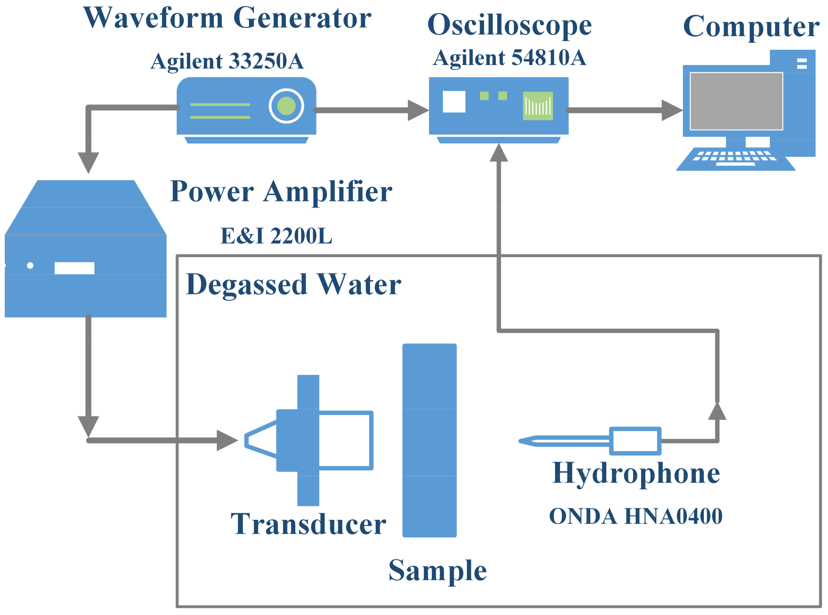
2.4.2. Experimental Setup

The thickness of each phantom sample was L_s = 42.3 mm, with a density of ρ₁ = 1000 kg/m³ so that it could stably suspend in the water. The distance between transducer and the phantom was 37.7 mm. Following the same protocol used in our previous work [45], the nonlinearity parameter was measured as β = 4.2. Since the only difference in gel recipe between the two works is the introduction of amino polystyrene microspheres in this paper, the same β value indicates that microspheres did not influence the nonlinear propagation of waves. To confirm this, we measured the ratio between the second harmonic and fundamental components, and found it was identical to that in [45] under the same sonication conditions. The attenuation coefficient and sound velocity of phantom, as functions of frequency, were measured through a broadband spectrum method [48,49]. In the measurement, two planar piston transducers (Immersion, Unfocused, Panametrics, Waltham, MA, USA) calibrated with a needle hydrophone (HNC-1000, ONDA Corp., Sunnyvale, CA, USA), were placed on the opposite sides of the phantom, with one of them driven by a broadband pulse generator (5900PR, Panametrics). The reflected and transmitted acoustic signals were then acquired by the transducers and digitalized with a digital oscilloscope (54830B, Agilent, Santa Clara, CA, USA). (Device connection was similar to that in [49]). In the measurements, 8 continuous pulse sequences were acquired and averaged to reduce the signal-to-noise ratio (SNR).

Prior to the HIFU experiments, a low-level driving voltage was used to drive a customized HIFU transducer (Chongqing Haifu Med. Tech. Co., Ltd., Chongqing, China) to emit a linear sound field. Simultaneously, effective parameters of the transducer, such as effective radius, radiation profile, and angle of divergence were obtained by adjusting the transducer parameters in the KZK calculations, such that the linear field predicted via KZK was consistent with that measured [45]. The effective parameters were then used in the simulations of both the KZK and mKZK models. As a result, the HIFU transducer (working frequency 1.12 MHz) had an effective aperture radius of 48.6 mm and a geometrical focal length of 101.5 mm. As illustrated in Figure 1, the transducer was immersed in water and driven with signals from a signal generator (33250A, Agilent, Santa Clara, CA, USA) amplified by a broadband power amplifier (2200L, E&I, Rochester, NY, USA). The input voltage was set as 465 mV (20 cycles; burst period, 10 ms; duty cycle, 0.18%). Another needle hydrophone (HNA-0400, ONDA Corp., Sunnyvale, CA, USA) was mounted on a customized three-dimensional (3D) scanning system (Controller Model: XPS-C8, Newport, CA, USA) to scan the HIFU field. To suppress possible acoustic cavitation in surrounding liquid, the water was processed with a self-developed water degassing and deionizing system. The temporal and spatial scanning procedure was controlled via the GPIB interface (National Instruments, Austin, TX, USA).

3. Results and Discussions

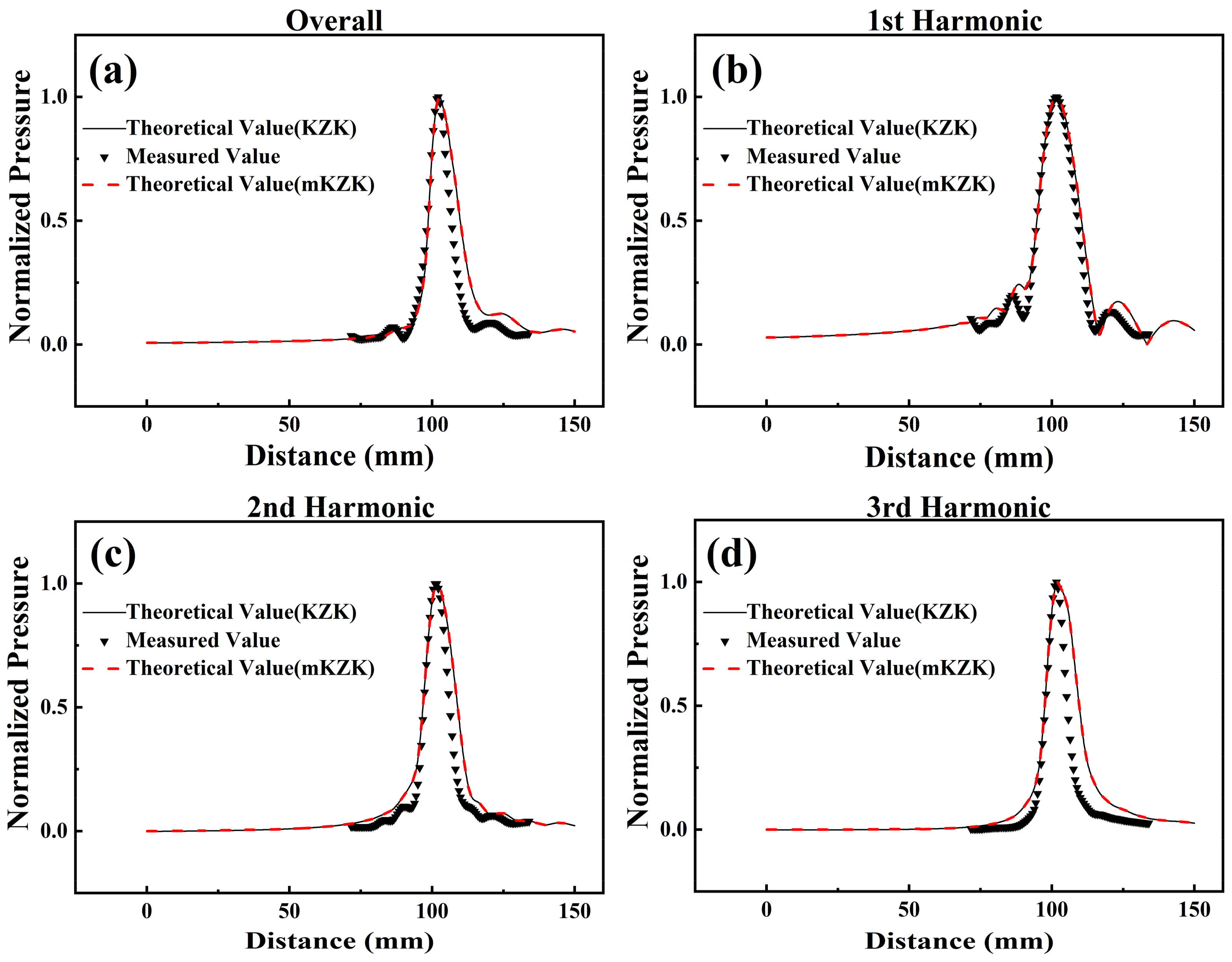
3.1. Non-Dispersive Water

In order to verify the validity of the modified model, the mKZK equation was used to predict the sound field distributions generated from the transducer. In this case, the media in the direction of propagation was degassed water, and the surface pressure of the transducer was set to be 0.4 MPa. Then, the results were compared with those obtained from experimental measurements as well as from the original KZK model. The results are presented in Figure 2 for comparison. Due to the axial-symmetry of the sound field, only the sound field distribution in the axial direction was studied. Also, since the major concern of this paper is to investigate how the focal-shift could be accurately predicted, the pressure profiles are all presented in a normalized way, so that the focal-shift effect is more intuitive and easy to observe. For the total pressure distributions presented in Figure 2a, the axial distribution of acoustic pressure seems identical for the modified and original KZK models, which provides reliable proof that the current theoretical modification did not compromise the accuracy of the sound field prediction in non-dispersive media. With the help of fast Fourier transform (FFT) algorithm, further analysis was then carried out by decomposing the total sound pressure into the superposition of linear and nonlinear components. In Figure 2b–d, all the components exhibited good agreement between the results calculated from the modified and the original KZK models, showing that both models are applicable for sound field prediction under the experimental conditions mentioned above. It should also be noted that, in Figure 2 the locations of the pressure peaks from the two models were exactly the same for all components, although the measured axial beam-widths seem a bit narrower than both theoretical predictions, especially for harmonic components. Since the linear fields were found to be almost identical for the measured and predicted results, we speculate that some far-field attenuation factors such as dissolved oxygen in water, or bubbles might exist. However, this does not affect the conclusion on the location of the maximum pressure.

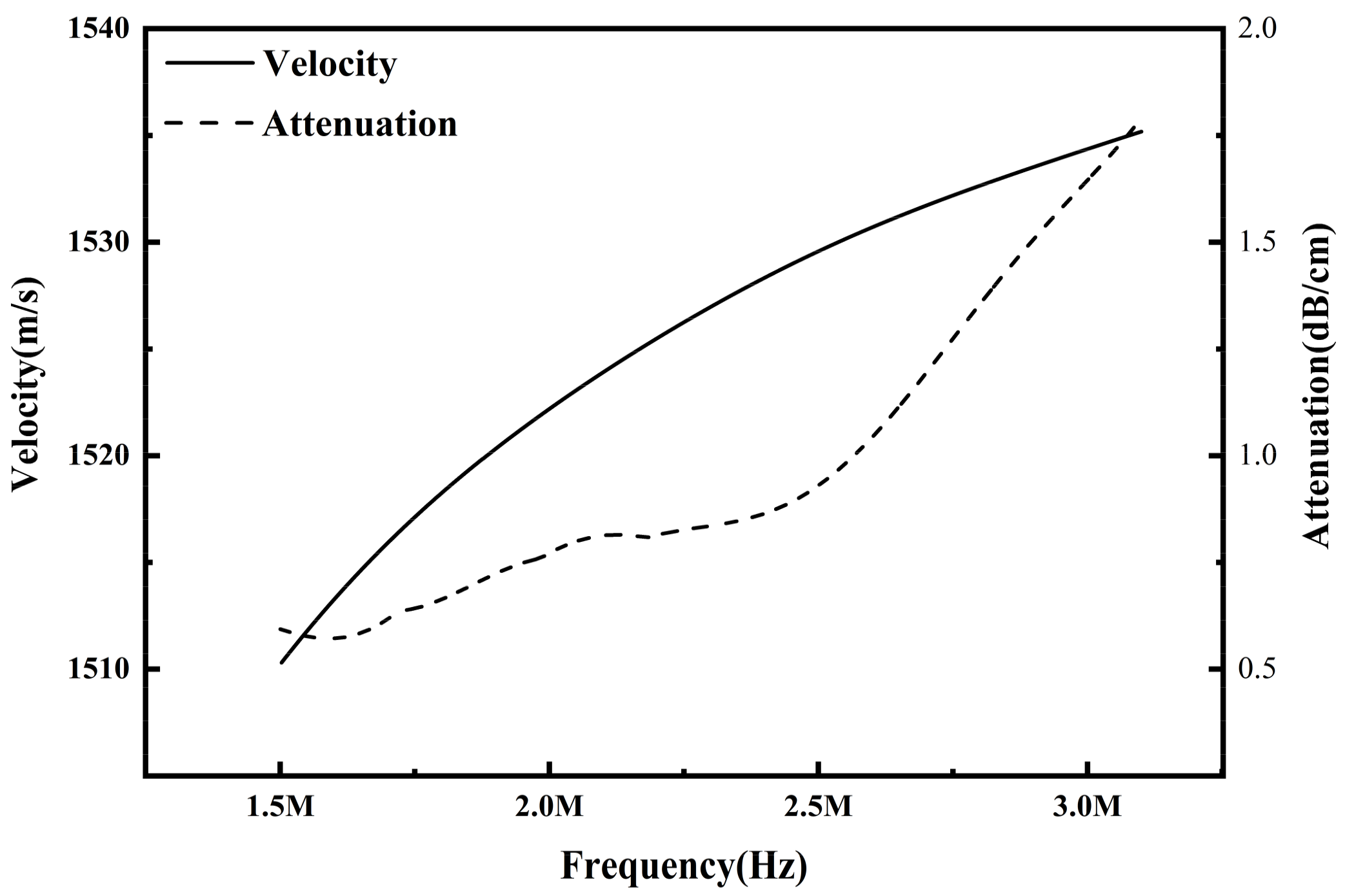
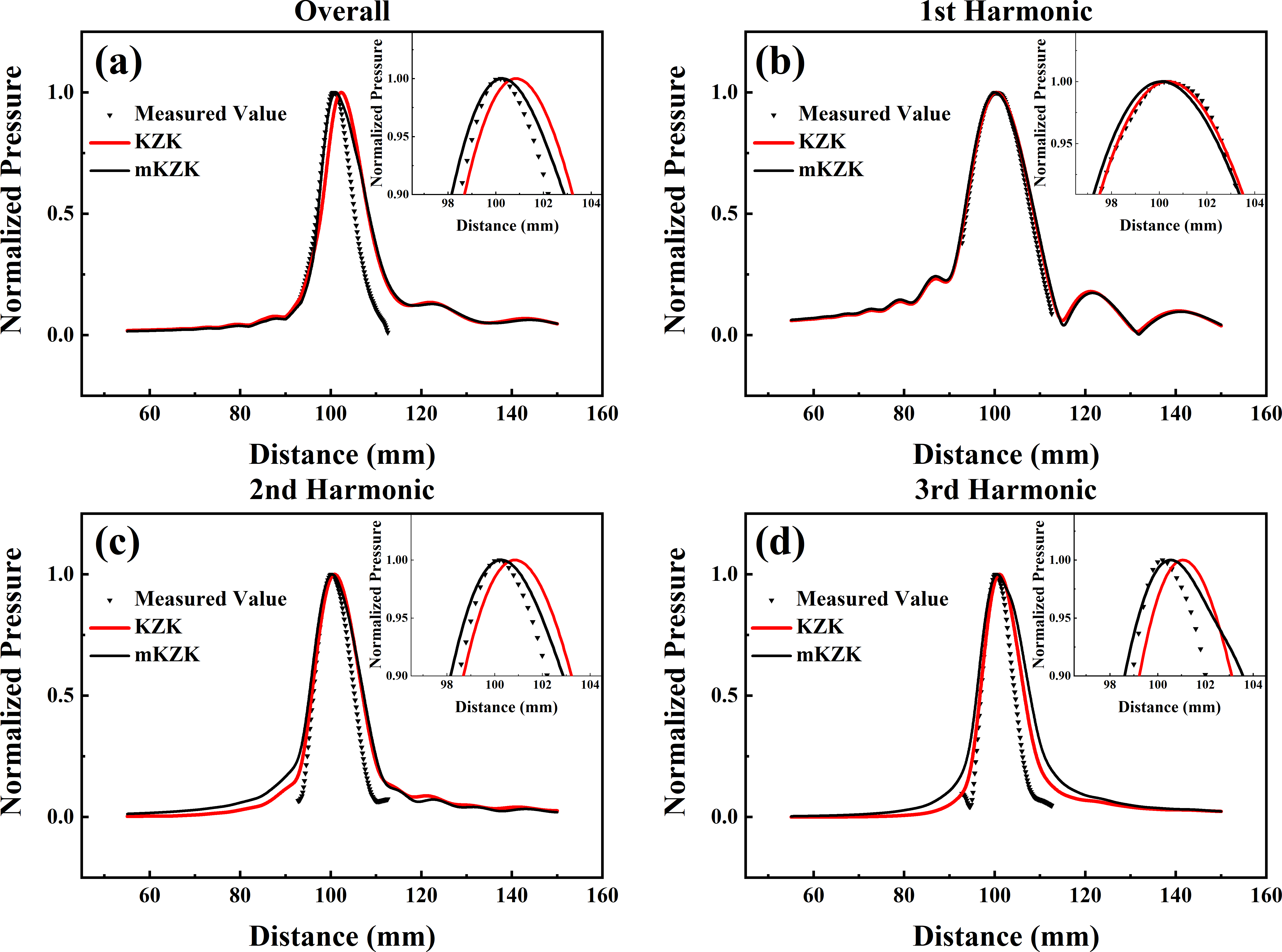
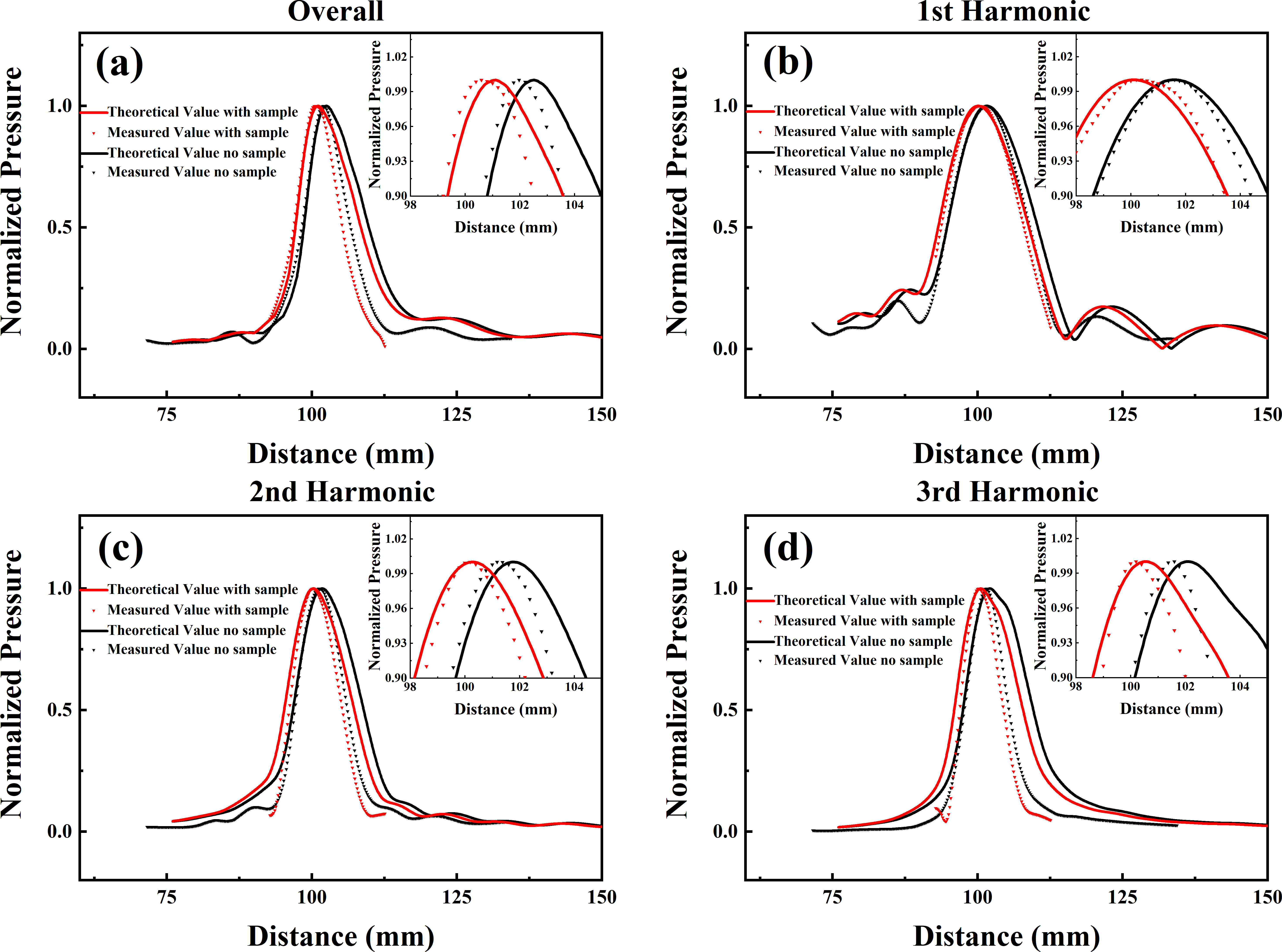
3.2. Dispersive Phantom

To incorporate the phantom model into the study, the acoustic parameters of the phantom was firstly characterized according to procedures described in earlier studies [48,49]. In brief, the acoustic phase velocity c(f) inside the phantom material was determined by [48]

$$c\left(f\right)=c_{\mathrm{w}}\left[1+2\frac{{\theta }_{\mathrm{w}}\left(f\right)-{\theta }_{\mathrm{s}}\left(f\right)}{{\theta }_2\left(f\right)-{\theta }_1\left(f\right)}\right],$$

(17)

where the sound velocity in water c_w was considered as 1500 m/s. When the sound velocity inside the phantom was measured, the acoustic signals p_s and p_f were the acoustic pressure acquired by a transducer before and after the phantom was inserted into the acoustic path. While p₁ and p₂ were the pressure of the reflected signals from the first and second water/phantom interfaces, respectively, θ_w(f), θ_s(f), θ₁(f) and θ₂(f) were the corresponding phase spectra. The frequency dependence of the attenuation coefficient α(f) was calculated according to [48,49]

$$\alpha \left(f\right)=\frac{1}{L_s}\left[\ln \left(\frac{A_1}{A_2}\right)-\ln \left(\frac{A_w}{A_s}\right)\right],$$

(18)

where A_w, A_s, A₁ and A₂ were the amplitude spectra corresponding to the above-mentioned phase responses. Figure 3 plots the measured attenuation coefficient and acoustic velocity as a function of frequency. In the frequency range 1.5–3.1 MHz, the sound velocity increased by about 26 m/s. The acoustic attenuation coefficient increased from 0.59 dB/cm at 1.5 MHz to 1.79 dB/cm at 3.1 MHz, indicating the attenuation factor being y = 1.83 for the phantom. The attenuation factor was obtained from the exponential fitting using a curve fitting toolbox in Matlab. It should be noted that sound velocity could fluctuate due to the thermal effect of focused ultrasound. However, in this work the duty cycle was as low as 0.18%, and a medium-level surface pressure of up to 0.4 MPa was chosen for the transducer. Thus, no significant temperature elevation was observed during the experiments, and the thermal-induced change in sound velocity could be neglected [50]. It should also be mentioned, that to account for the thermal-effect, an appropriate bio-heat transferring equation should be incorporated with the current model. The main concern then lies in the dispersion due to microsphere scattering. In clinical applications, the major dispersion originates from tissues like fat, whose attenuation coefficient is generally larger than that of body tissue. Therefore, in comparison with other research in which the parameters of the phantom were nearly the same as body tissue (e.g., liver and spleen), the choice of phantoms with larger attenuation coefficients in the present experiments might provide results in better agreement with the actual situation. Meanwhile, since the measured physical parameters are close to those of dense fat, this setup could be regarded as a simplified mimic of the abdomen in HIFU therapies.

As is illustrated in Figure 4, the acoustic field distribution along the axial direction is examined by sitting the phantom on the acoustic path of the transducer. The results show the comparison between measured data and simulated results obtained from both the modified and traditional KZK models. Figure 4a describes the total pressure and Figure 4b–d shows the fundamental, second harmonic and third harmonic components, respectively. For the total pressure distribution, it is clearly observed that the peak-pressure location predicted through the mKZK model agrees well with that acquired in experiments, while the data calculated from the traditional KZK model show a deviation from the previous two groups. Note that the axial peak-pressure deviation is quite small for the fundamental components, but it gradually becomes significant when more harmonic components appear. Thus, the overall peak-pressure deviation observed in Figure 4a is mainly caused by higher-order harmonic components, indicating that the significance of the theoretical modification relies on high nonlinearity, such as in HIFU. This phenomenon could be addressed with the results shown in Figure 3, where higher-order harmonic waves that occupy higher frequency bands exhibit more notable sound velocity/attenuation dispersions, thus play a more dominant role in the modification of the KZK model. Meanwhile, it can be seen from Figure 4 that the modified equation has larger variation than the KZK equation. The effect of the mKZK equation on the simulation results can be thus clarified as providing more precise prediction for experimental results. The results in Figure 4 give persuasive proof that theoretical modifications made previously are necessary and valid. The beam narrowing effect caused by data normalization still exists. However, in actual treatment more attention is paid to the location of the focus point, because the location determines the heat distribution area, which significantly alters the biological properties of the treatment area.

Among existing studies, most researchers have focused on the thermos-lensing effect [23] and bubble formation induced focal region distortion [25,26], while some also mentioned the acoustic radiation force induced tissue displacement [27]. With the results presenting the dispersion of sound velocity and attenuation in tissues, the deviation of focal spots can be well explained in combination with the strong nonlinearity nature of HIFU.

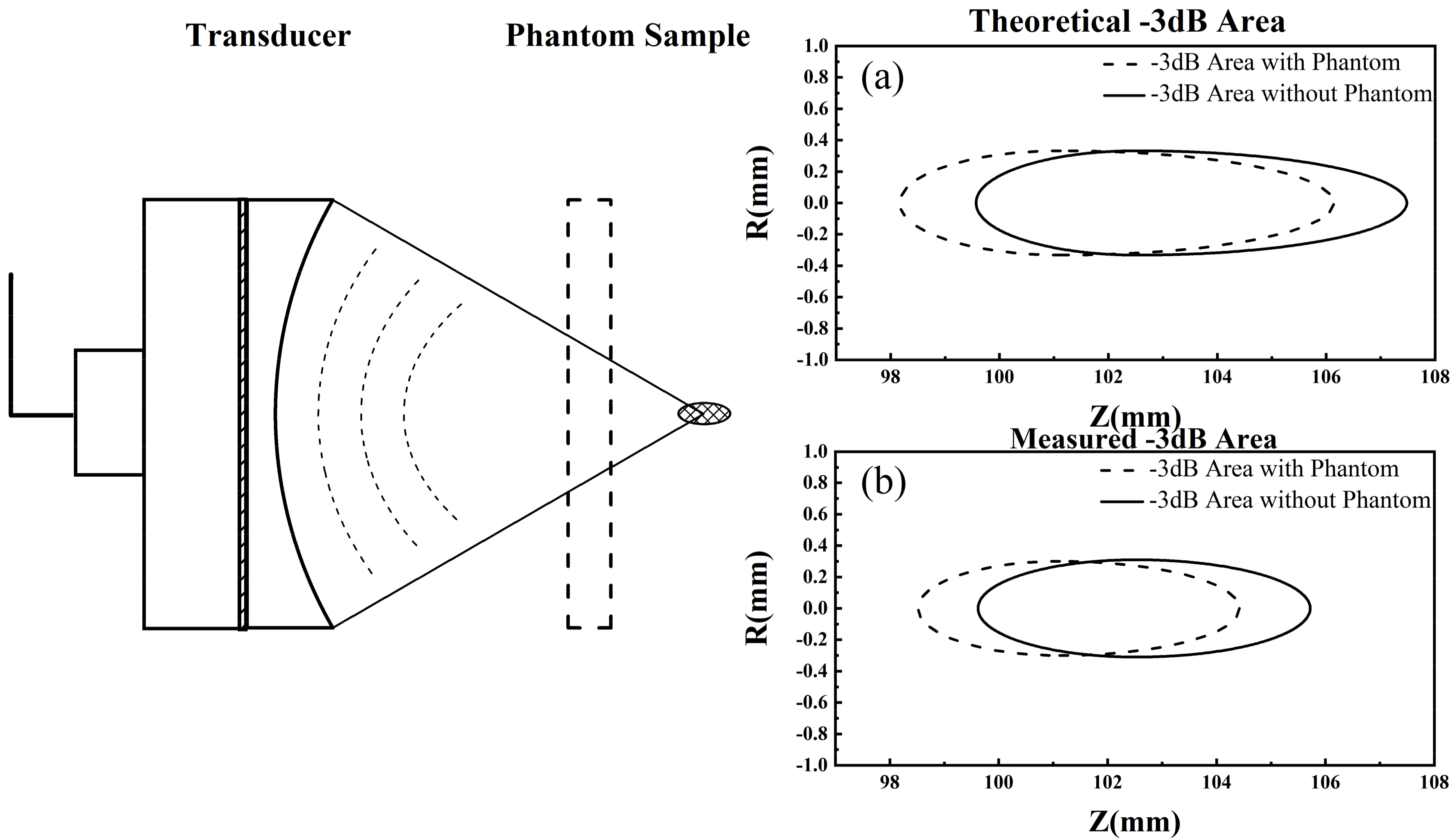
3.3. Dispersion-Induced Focus Shift

It is of great importance to evaluate how the mKZK model demonstrates its significance in HIFU applications. In Figure 5, comparisons are carried out to display how the wave distribution behaves differently before and after inserting the phantom sample into the wave propagation path. It can be observed that, for either data from experiments or from the mKZK model, although only a slight difference is seen in the axial wave profile when examining the fundamental components, an axial focus shift is more evident for the overall acoustic pressure since it is highly affected by the harmonic components. It is explained here that, due to the dispersive nature of the phantom, higher-order harmonic components require larger values of both sound velocity and attenuation coefficient in the KZK model, urging the overall wave profile to move forward to the transducer.

In the present study, the focus shift distance was quantified for the overall axial acoustic pressure distribution and its decomposed components, and this is listed in

Table 1. Focus shift induced by acoustic-dispersive phantom sample (in mm).

Method	Overall	Fundamental	2nd Harmonic	3rd Harmonic
mKZK	1.47	1.41	1.51	1.62
Experiment	1.42 ± 0.04	1.40 ± 0.03	1.45 ± 0.04	1.51 ± 0.04

.

The focus shift, which is found to be of millimeter magnitude for the studied condition, cannot be ignored, especially for clinical HIFU studies. On the one hand, in typical HIFU applications, the much higher surface pressure would induce even stronger acoustic nonlinearity in the focus area, and up to tens of orders of harmonic components might contribute to the overall acoustic responses. In that case, dispersion in acoustic velocity as well as the attenuation coefficient could cause larger focus shifts. On the other hand, even for the millimeter-level focus shift exhibited with the current setup, an impressive amount of acoustic energy would be deposited outside the designated focus area. As demonstrated in Figure 6, about 25% of the −3 dB focal region would fall outside of the one predicted by the traditional KZK equation, when the phantom sample is introduced into the transducer axis. In addition, the absence of shockwaves in the experiment should be noted, and this indicates that the influence of shockwaves could be ignored in the theoretical model under such experimental parameters.

3.4. Discussion

In previous studies, shifts between the predicted and observed focal regions have been frequently reported in HIFU-related studies. Usually, the shift was measured to be around 1–3 mm for 1-MHz HIFU transducers [24], 4–5 mm for ~2.2-MHz excitation [51], and an empirical formula was also used to calculate the focus shift [22]. Although different possible mechanisms have been proposed and a series of correlation studies have been carried out [21,22,23,24,25,26,27], detailed theoretical proof that could quantitatively explain the inherent mechanisms of the observed focal shifts is still lacking. The proposed model modification here clarifies how the acoustic dispersion played a role in the complicated physics of this problem.

The experiments carried out here have demonstrated that the observed focal shift should come from the dispersive behavior of sound velocity and attenuation in media. For different harmonic components in the HIFU beam, their sound velocities could be different at the gel/water interface. Speculating from Snell’s law, these different components could actually propagate along slightly different paths in the phantom, causing the focal point to shift its location. That is also why the main difference between the two models is observed for the harmonics in Figure 4 and Figure 5—because the sound velocity of the harmonics deviated further away as their frequencies were higher. During this process, the attenuation should also have contributed in a dispersive way. However, the influence of dispersive attenuation could not be separated from that of sound velocity.

Despite the general recognition that the Westervelt equation and SBE provide higher precision in non-dispersive sound field prediction than KZK, difficulties in predicting accurate sound field distribution in strong dispersion media still remains a great challenge [22]. Moreover, due to the existing complexity of the Westervelt equation and SBE, adding more modifications to these two equations could be over-whelming and/or time-consuming for clinical applications that require real-time monitoring. Considering that KZK shows a balance between accuracy and computation burden, this paper chose to further modify the KZK equation as a straightforward way to achieve improved simulation of HIFU propagation, especially to work out how the focal-shift could be predicted accurately. In this work, for consistency of the experiment, the mKZK and KZK in ordinary media was first confirmed. Then, when measuring the parameters in the strong dispersion medium, mKZK gave a more accurate prediction of the focal shift. Thus, by using the mKZK equation we can quickly and accurately predict the HIFU field in complex media.

However, further theoretical studies are still needed since the current model is unable to eradicate all the possible unfavorable factors in predicting the characteristics of HIFU. For example, defocusing effects or shifts in focal position might be caused by the layered tissue effect, where sound speed/attenuation may vary in different tissues layers. The thermal lesion effect, in which the tissue properties change due to the heating of HIFU, could be more difficult to include in the modeling. A full solution could be even more challenging if other possible mechanisms, including acoustic radiation force, acoustic cavitation and inconsistent thermal deposition [27] are also considered.

The focal shifts observed in phased-array-based HIFU devices are also notable. For instance, a focal shift of about 2-mm was observed along the transducer axis in multiple-layered soft tissues sonicated with a 65-element phased array transducer [22]. To overcome this problem in phased-array HIFU, possible solutions could be obtained by drawing lessons from the underlying mechanisms discussed above.

4. Conclusions

Although HIFU technology based on the KZK equation calculation has been widely accepted and used in the clinical setting and transducer designs, the absence of an accurate theory to predict the sound field inevitably limits the application of the ultrasound focusing. In this work, a mKZK equation is proposed to predict the HIFU field established with a spherical focusing transducer. Meanwhile, the accuracy of the methods is verified through experiment. This method could improve the computational accuracy of the KZK equation in dispersive media, which is similar to human tissue. Simulation and experimental results show that the focus area will shift towards the transducer and the offset increases as the nonlinearity becomes higher. Therefore, in the process of HIFU transducer design, the impact of dispersion on the results need to be taken into account, in order that accurate sonication can be achieved. By modifying the KZK equation, the findings will help with transducer design and the application of the HIFU. This will also help to ensure the stability and safety of HIFU and further accelerate its clinical applications.

References

1. Lynn, J.G.; Zwemer, R.L.; Chick, A.J.; Miller, A.E. A new method for the generation and use of focused ultrasound in experimental biology. J. Gen. Physiol. 1942, 26, 179. [Google Scholar] [CrossRef] [PubMed]
2. Fry, W.J.; Fry, F.; Barnard, J.; Krumins, R.; Brennan, J. Ultrasonic lesions in mammalian central nervous system. Science 1955, 122, 1091. [Google Scholar] [CrossRef]
3. Westervelt, P.J. Parametric acoustic array. J. Acoust. Soc. Am. 1963, 35, 535–537. [Google Scholar] [CrossRef]
4. Hallaj, I.M.; Cleveland, R.O. FDTD simulation of finite-amplitude pressure and temperature fields for biomedical ultrasound. J. Acoust. Soc. Am. 1999, 105, L7–L12. [Google Scholar] [CrossRef] [PubMed]
5. Zabolotskaya, E. Quasi-plane waves in the nonlinear acoustics of confined beams. Sov. Phys. Acoust. 1969, 15, 35–40. [Google Scholar]
6. Kuznetsov, V. Equation of nonlinear acoustics. Sov. Phys. Acoust. 1971, 16, 467–470. [Google Scholar]
7. Tjotta, J.N.; Tjotta, S.; Vefring, E.H. Effects of focusing on the nonlinear interaction between two collinear finite amplitude sound beams. J. Acoust. Soc. Am. 1991, 89, 1017–1027. [Google Scholar] [CrossRef]
8. Kamakura, T.; Ishiwata, T.; Matsuda, K. Model equation for strongly focused finite-amplitude sound beams. J. Acoust. Soc. Am. 2000, 107, 3035–3046. [Google Scholar] [CrossRef] [PubMed]
9. Kamakura, T.; Ishiwata, T.; Matsuda, K. A new theoretical approach to the analysis of nonlinear sound beams using the oblate spheroidal coordinate system. J. Acoust. Soc. Am. 1999, 105, 3083–3086. [Google Scholar] [CrossRef]
10. ter Haar, G. Biological effects of ultrasound in clinical applications. In Ultrasound: Its Chemical, Physical and Biological Effects; VCH Publishers: New York, NY, USA, 1988. [Google Scholar]
11. ter Haar, G. Turning up the power: High intensity focused ultrasound (HIFU) for the treatment of cancer. Ultrasound 2007, 15, 73–77. [Google Scholar] [CrossRef]
12. Wu, F.; Chen, W.-Z.; Bai, J.; Zou, J.-Z.; Wang, Z.-L.; Zhu, H.; Wang, Z.-B. Pathological changes in human malignant carcinoma treated with high-intensity focused ultrasound. Ultrasound Med. Biol. 2001, 27, 1099–1106. [Google Scholar] [CrossRef]
13. Gelet, A.; Chapelon, J.; Bouvier, R.; Rouviere, O.; Lasne, Y.; Lyonnet, D.; Dubernard, J. Transrectal high-intensity focused ultrasound: Minimally invasive therapy of localized prostate cancer. J. Endourol. 2000, 14, 519–528. [Google Scholar] [CrossRef] [PubMed]
14. Orsi, F.; Arnone, P.; Chen, W.; Zhang, L. High intensity focused ultrasound ablation: A new therapeutic option for solid tumors. J. Cancer Res. Ther. 2010, 6, 414. [Google Scholar] [CrossRef] [PubMed]
15. Illing, R.; Kennedy, J.; Wu, F.; ter Haar, G.; Protheroe, A.; Friend, P.; Gleeson, F.; Cranston, D.; Phillips, R.; Middleton, M. The safety and feasibility of extracorporeal High-Intensity Focused Ultrasound (HIFU) for the treatment of liver and kidney tumours in a Western population. Br. J. Cancer 2005, 93, 890. [Google Scholar] [CrossRef] [PubMed]
16. Zhou, Y.-F. High intensity focused ultrasound in clinical tumor ablation. World J. Clin. Oncol. 2011, 2, 8. [Google Scholar] [CrossRef] [PubMed]
17. Gudur, M.S.R.; Kumon, R.E.; Zhou, Y.; Deng, C.X. High-frequency rapid B-mode ultrasound imaging for real-time monitoring of lesion formation and gas body activity during high-intensity focused ultrasound ablation. IEEE Trans. Ultrason. Ferroelectr. Freq. Control 2012, 59, 1687–1699. [Google Scholar] [CrossRef] [PubMed]
18. Kemmerer, J.; Ghoshal, G.; Oelze, M. Quantitative ultrasound assessment of HIFU induced lesions in rodent liver. In Proceedings of the 2010 IEEE International Ultrasonics Symposium, San Diego, CA, USA, 11–14 October 2010; pp. 1396–1399. [Google Scholar]
19. Wijlemans, J.; Bartels, L.; Deckers, R.; Ries, M.; Mali, W.T.M.; Moonen, C.; Van Den Bosch, M. Magnetic resonance-guided high-intensity focused ultrasound (MR-HIFU) ablation of liver tumours. Cancer Imaging 2012, 12, 387. [Google Scholar] [CrossRef] [PubMed]
20. Zhang, L.; Chen, W.; Liu, Y.; Hu, X.; Zhou, K.; Chen, L.; Peng, S.; Zhu, H.; Zou, H.; Bai, J. Feasibility of magnetic resonance imaging-guided high intensity focused ultrasound therapy for ablating uterine fibroids in patients with bowel lies anterior to uterus. Eur. J. Radiol. 2010, 73, 396–403. [Google Scholar] [CrossRef] [PubMed]
21. Petrusca, L.; Viallon, M.; Breguet, R.; Terraz, S.; Manasseh, G.; Auboiroux, V.; Goget, T.; Baboi, L.; Gross, P.; Sekins, K.M. An experimental model to investigate the targeting accuracy of MR-guided focused ultrasound ablation in liver. J. Transl. Med. 2014, 12, 12. [Google Scholar] [CrossRef] [PubMed]
22. Li, D.; Shen, G.; Bai, J.; Chen, Y. Focus shift and phase correction in soft tissues during focused ultrasound surgery. IEEE Trans. Biomed. Eng. 2011, 58, 1621–1628. [Google Scholar] [CrossRef] [PubMed]
23. Connor, C.W.; Hynynen, K. Bio-acoustic thermal lensing and nonlinear propagation in focused ultrasound surgery using large focal spots: A parametric study. Phys. Med. Biol. 2002, 47, 1911. [Google Scholar] [CrossRef] [PubMed]
24. Meaney, P.M.; Cahill, M.D.; ter Haar, G. The intensity dependence of lesion position shift during focused ultrasound surgery. Ultrasound Med. Biol. 2000, 26, 441–450. [Google Scholar] [CrossRef]
25. Zderic, V.; Foley, J.; Luo, W.; Vaezy, S. Prevention of post-focal thermal damage by formation of bubbles at the focus during high intensity focused ultrasound therapy. Med. Phys. 2008, 35, 4292–4299. [Google Scholar] [CrossRef] [PubMed]
26. Zhou, Y.; Wilson Gao, X. Variations of bubble cavitation and temperature elevation during lesion formation by high-intensity focused ultrasound. J. Acoust. Soc. Am. 2013, 134, 1683–1694. [Google Scholar] [CrossRef] [PubMed]
27. Laughner, J.I.; Sulkin, M.S.; Wu, Z.; Deng, C.X.; Efimov, I.R. Three potential mechanisms for failure of high intensity focused ultrasound ablation in cardiac tissue. Circulation 2012, 5, 409–416. [Google Scholar] [CrossRef] [PubMed]
28. Bobkova, S.; Gavrilov, L.; Khokhlova, V.; Shaw, A.; Hand, J. Focusing of high-intensity ultrasound through the rib cage using a therapeutic random phased array. Ultrasound Med. Biol. 2010, 36, 888–906. [Google Scholar] [CrossRef] [PubMed]
29. Liu, Z.; Fan, T.; Zhang, D.; Gong, X. Influence of the abdominal wall on the nonlinear propagation of focused therapeutic ultrasound. Chin. Phys. B 2009, 18, 4932–4937. [Google Scholar]
30. Rosnitskiy, P.B.; Yuldashev, P.V.; Sapozhnikov, O.A.; Maxwell, A.D.; Kreider, W.; Bailey, M.R.; Khokhlova, V.A. Design of HIFU Transducers for Generating Specified Nonlinear Ultrasound Fields. IEEE Trans. Ultrason. Ferroelectr. Freq. Control 2017, 64, 374–390. [Google Scholar] [CrossRef] [PubMed]
31. Soneson, J.E. A parametric study of error in the parabolic approximation of focused axisymmetric ultrasound beams. J. Acoust. Soc. Am. 2012, 131, EL481–EL486. [Google Scholar] [CrossRef] [PubMed]
32. O’Donnell, M.; Jaynes, E.; Miller, J. Kramers-Kronig relationship between ultrasonic attenuation and phase velocity. J. Acoust. Soc. Am. 1981, 69, 696–701. [Google Scholar] [CrossRef]
33. Kudo, N.; Kamataki, T.; Yamamoto, K.; Onozuka, H.; Mikami, T.; Kitabatake, A.; Ito, Y.; Kanda, H. Ultrasound attenuation measurement of tissue in frequency range 2.5–40 MHz using a multi-resonance transducer. In Proceedings of the Ultrasonics Symposium, Toronto, ON, Canada, 5–8 October 1997; pp. 1181–1184. [Google Scholar]
34. Wojcik, G.; Mould, J.; Abboud, N.; Ostromogilsky, M.; Vaughan, D. Nonlinear modeling of therapeutic ultrasound. In Proceedings of the Ultrasonics Symposium, Seattle, WA, USA, 7–10 November 1995; pp. 1617–1622. [Google Scholar]
35. Makris, N.; Constantinou, M. Fractional-derivative Maxwell model for viscous dampers. J. Struct. Eng. 1991, 117, 2708–2724. [Google Scholar] [CrossRef]
36. Szabo, T.L. Time domain wave equations for lossy media obeying a frequency power law. J. Acoust. Soc. Am. 1994, 96, 491–500. [Google Scholar] [CrossRef]
37. Szabo, T.L. Causal theories and data for acoustic attenuation obeying a frequency power law. J. Acoust. Soc. Am. 1995, 97, 14–24. [Google Scholar] [CrossRef]
38. Szabo, T.L.; Wu, J. A model for longitudinal and shear wave propagation in viscoelastic media. J. Acoust. Soc. Am. 2000, 107, 2437–2446. [Google Scholar] [CrossRef] [PubMed]
39. Treeby, B.E.; Jaros, J.; Rendell, A.P.; Cox, B.T. Modeling nonlinear ultrasound propagation in heterogeneous media with power law absorption using a k-space pseudospectral method. J. Acoust. Soc. Am. 2012, 131, 4324–4336. [Google Scholar] [CrossRef] [PubMed]
40. Prieur, F.; Holm, S. Nonlinear acoustic wave equations with fractional loss operators. J. Acoust. Soc. Am. 2011, 130, 1125–1132. [Google Scholar] [CrossRef] [PubMed]
41. Rosnitskiy, P.B.; Yuldashev, P.V.; Vysokanov, B.A.; Khokhlova, V.A. Setting boundary conditions on the Khokhlov-Zabolotskaya equation for modeling ultrasound fields generated by strongly focused transducers. Acoust. Phys. 2016, 62, 151–159. [Google Scholar] [CrossRef]
42. Heymans, N.; Podlubny, I. Physical interpretation of initial conditions for fractional differential equations with Riemann-Liouville fractional derivatives. Rheol. Acta 2006, 45, 765–771. [Google Scholar] [CrossRef]
43. Zhao, X.; McGough, R.J. The Khokhlov-Zabolotskaya-Kuznetsov (KZK) equation with power law attenuation. In Proceedings of the IEEE International Ultrasonics Symposium, Chicago, IL, USA, 3–6 September 2014; pp. 2225–2228. [Google Scholar]
44. Kelly, J.F.; McGough, R.J.; Meerschaert, M.M. Analytical time-domain Green’s functions for power-law media. J. Acoust. Soc. Am. 2008, 124, 2861–2872. [Google Scholar] [CrossRef] [PubMed]
45. Fan, T.; Liu, Z.; Zhang, D.; Tang, M. Comparative study of lesions created by high-intensity focused ultrasound using sequential discrete and continuous scanning strategies. IEEE Trans. Biomed. Eng. 2013, 60, 763–769. [Google Scholar] [CrossRef] [PubMed]
46. Fan, T.; Zhang, D.; Gong, X. Estimation of the tissue lesion induced by a transmitter with aluminium lens. J. Phys. 2011, 279, 012020. [Google Scholar] [CrossRef]
47. Lafon, C.; Zderic, V.; Noble, M.L.; Yuen, J.C.; Kaczkowski, P.J.; Sapozhnikov, O.A.; Chavrier, F.; Crum, L.A.; Vaezy, S. Gel phantom for use in high-intensity focused ultrasound dosimetry. Ultrasound Med. Biol. 2005, 31, 1383–1389. [Google Scholar] [CrossRef] [PubMed]
48. He, P. Measurement of acoustic dispersion using both transmitted and reflected pulses. J. Acoust. Soc. Am. 2000, 107, 801–807. [Google Scholar] [CrossRef] [PubMed]
49. He, P.; Zheng, J. Acoustic dispersion and attenuation measurement using both transmitted and reflected pulses. Ultrasonics 2001, 39, 27–32. [Google Scholar] [CrossRef]
50. Fan, T.; Zhang, D.; Zhang, Z.; Ma, Y.; Gong, X. Effects of vapour bubbles on acoustic and temperature distributions of therapeutic ultrasound. Chin. Phys. B 2008, 17, 3372–3377. [Google Scholar] [CrossRef]
51. Camarena, F.; Adrián-Martínez, S.; Jiménez, N.; Sánchez-Morcillo, V. Nonlinear focal shift beyond the geometrical focus in moderately focused acoustic beams. J. Acoust. Soc. Am. 2013, 134, 1463–1472. [Google Scholar] [CrossRef] [PubMed]
Figure 1. The experimental setup.
Applsci 08 00609 g001
Figure 2. The normalized acoustic pressure distributions along the axis of the HIFU transducer without the phantom: (a) the overall pressure; (b) the fundamental component; (c) the second harmonic; (d) the third harmonic.
Applsci 08 00609 g002
Figure 3. Measured frequency-dependent acoustic velocity and attenuation coefficient of the phantom sample.
Applsci 08 00609 g003
Figure 4. The normalized acoustic pressure distributions along the axis of the HIFU transducer, with the phantom placed at 37.7 mm away from the transducer. (a) the overall pressure; (b) the fundamental component; (c) the second harmonic; (d) the third harmonic.
Applsci 08 00609 g004
Figure 5. Comparison of the axial distributed acoustic pressure between the cases of with and without the phantom sample: (a) the overall pressure; (b) the fundamental component; (c) the second harmonic; (d) the third harmonic.
Applsci 08 00609 g005
Figure 6. Illustration of the focus shift induced by the presence of phantom sample: (a) the theoretical −3 dB area; (b) the measured −3 dB area.
Applsci 08 00609 g006