Application of Elastic Wave Velocity for Estimation of Soil Depth

1
Department of Civil Engineering, Kyung Hee University, Yongin 17-104, Korea
2
Department of Civil Engineering, Seoul National University of Science and Technology, Seoul 139-743, Korea
3
Department of Construction and Disaster Prevention Engineering, Daejeon University, Daejeon 300-716, Korea
*
Author to whom correspondence should be addressed.
Appl. Sci. 2018, 8(4), 600; https://doi.org/10.3390/app8040600
Submission received: 21 March 2018
/
Revised: 3 April 2018
/
Accepted: 5 April 2018
/
Published: 11 April 2018
(This article belongs to the Special Issue Modelling, Simulation and Data Analysis in Acoustical Problems)
Abstract
:Because soil depth is a crucial factor for predicting the stability at landslide and debris flow sites, various techniques have been developed to determine soil depth. The objective of this study is to suggest the graphical bilinear method to estimate soil depth through seismic wave velocity. Seismic wave velocity rapidly changes at the interface of two different layers due to the change in material type, packing type, and contact force of particles and thus, it is possible to pick the soil depth based on seismic wave velocity. An area, which is susceptible to debris flow, was selected, and an aerial survey was performed to obtain a topographic map and digital elevation model. In addition, a seismic survey and a dynamic cone penetration test were performed in this study. The comparison between the soil depth based on dynamic cone tests and the graphical bilinear method shows good agreement, indicating that the newly suggested soil depth estimating method may be usefully applied to predict soil depth.
1. Introduction
In assessing the stability of landslide or debris flow areas, both hydrological and geotechnical properties are the key parameters [1,2,3,4,5,6] among the various geotechnical properties such as soil strength, hydraulic conductivity, and friction angle, the soil depth is the most important parameter because the capacity for inflow and outflow of water is related to the soil thickness. Note that soil depth can be defined as the thickness of the soil from ground surface to consolidated medium [7,8].
The most reliable method to estimate soil depth at a given location is the test pit method, which involves direct excavation of a testing site in a square shape. However, excavation of multiple pits for the estimation of soil depth is very expensive and time-consuming. To overcome these limitations, Ref. [9] used a cone-tipped metal probe with a diameter of 18 mm for estimating local soil depth based on probe penetration resistance. Note that the methods mentioned above can only be performed at the selected local points; therefore, the soil depth of unmeasured areas is assumed to be the same as the measured depth of nearby points. However, soil depth shows substantial spatial variation; thus, the reliability of the above methods may be low, leading to the development of several models that consider the spatial distribution of soil depth. Ref. [10] developed the regolith-mantle slope method to predict the thickness of original parent material on a slope. Ref. [11] estimated soil depth based on the mass balance between soil production from underlying bedrock and divergence of diffusive soil transport. Even though these models are advantageous for obtaining soil depth across the whole area, the use of these models may not be easy because they require detailed information regarding hydrological, geotechnical, and geochemical parameters. Therefore, the geophysical method has been widely applied to estimate soil depth because it can quickly and cost-effectively provide various soil characteristics across an entire area. Electromagnetic waves have been used to measure electrical resistivity [12] and electrical conductivity [2], and the measured values can be converted into soil depths. Refs. [13,14] used seismic survey to predict soil depth and however, the studies merely showed the distributions of results without methodological content for picking soil depth. In addition, the applied previous geophysical methods require special reference values to determine soil depth and additional invasive experiments to enhance the reliability of the estimated soil depth.
This study proposes a graphical bilinear method to estimate soil depth based only on seismic survey. A seismic survey was performed, and the dynamic cone penetration test (DCPT) was also used to verify the soil depths deduced by the suggested technique. The measured information, including geological map, location, particle distribution, and distribution of seismic wave velocity were introduced first. Then the graphical bilinear method for determining soil depth, is demonstrated. The estimated soil depths using the suggested method are compared with values deduced by the dynamic cone penetration tests and their reliability is assessed.
2. Testing Site
2.1. Site Description
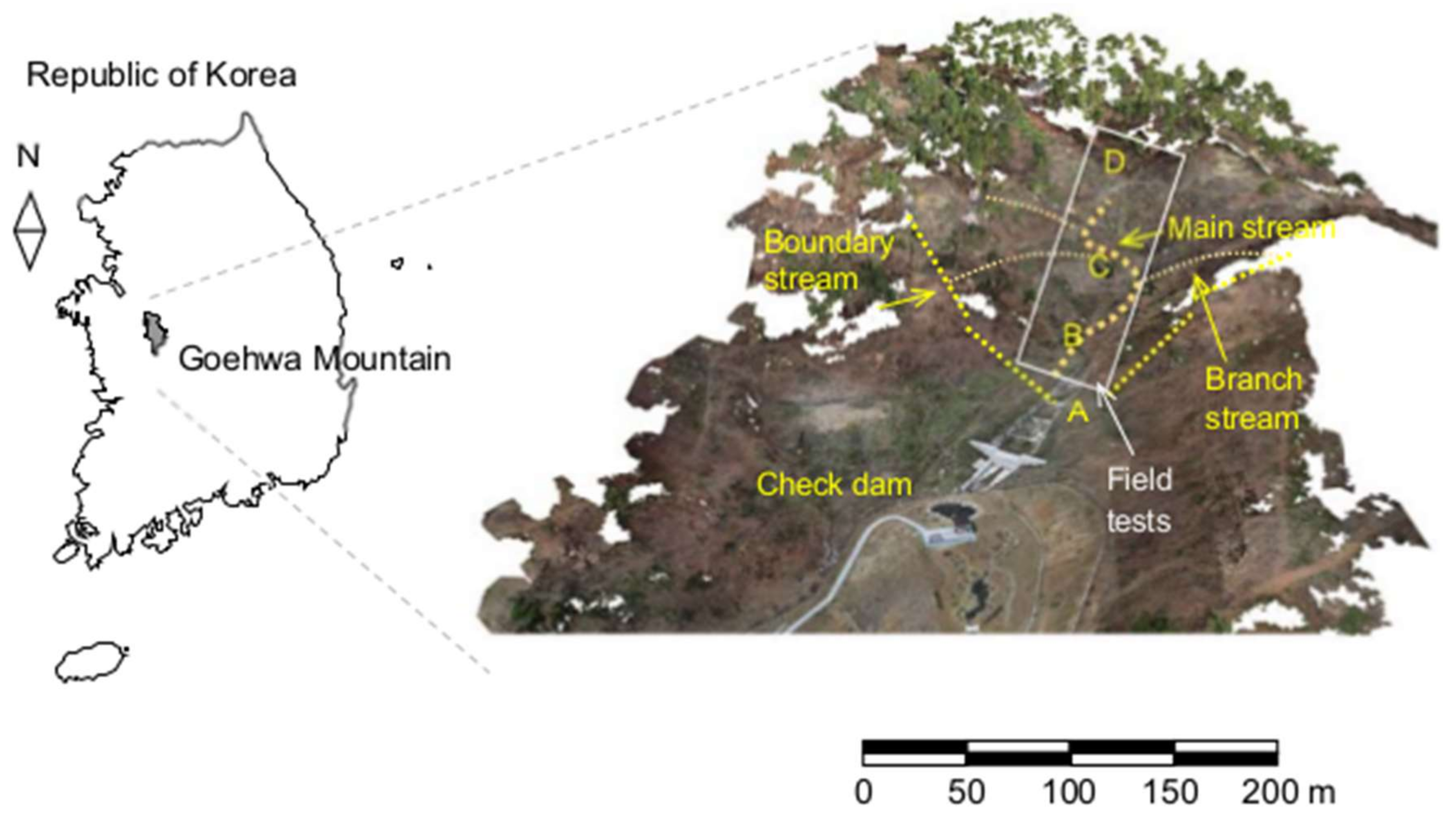
The selected testing site experienced debris flow a few years ago and is still susceptible to additional debris flow because of several geological characteristics of the site, including steep slope angle (over 32°) and saturated soil condition on slope. According to the geological map issued by the Korea Institute of Geology, Analysis, Mining (KIGAM), the testing area mainly consists of gneissose granite terrane. The testing site belongs to Mt. Geohwa, South Korea, where the altitude and area are approximately 200 m and 1.2 km2, respectively, and the latitude and longitude of the top of the mountain are N 36°29′15.7313′′ and E 127°18′40.5986′′. A drone aerial survey was performed to obtain a topographic map and digital elevation model. Figure 1 shows the topographic map: the area consists of one main stream and several branch streams. The vertical length and area of the main stream are approximately 206 m and 14,675 m2, respectively. Figure 1 also indicates the presence of the debris barrier and check dam at the site to prevent additional debris flow (N 36°29′04.3147′′, E 127°18′44.7017′′). The main stream was divided at four points, selected by considering slope characteristics: point A (N 36°29′10.8530′′, E 127°18′44.1891′′), point B (N 36°29′12.045′′, E 127°18′39.5912′′), point C (N 36°29′14.8329′′, E 127°18′30.7079′′), and point D (N 36°29′18.2046′′, E 127°18′23.6158′′). Point A, which is located at the bottom of the main stream, shows various fallen trees and weeds undergoing decay and rot, suggesting that considerable time has passed since the occurrence of the last debris flow. The slope of point A was measured to be approximately 10°, which is low compared to the slopes at points B and C. Thus, point A is covered with various flowed materials from the streams above due to debris flow. Point B shows a dramatically steeper slope of approximately 27° and the area mainly consists of sedimentary basin. Point C has the largest rapid slope (~32°) and width (maximum 105 m) among the selected points. Note that point C is located at a large catchment basin. Finally, point D indicates the initial zone where the debris flow occurred as ascertained by the presence of upright trees and a stable subsurface without collapsed conditions.
2.2. Soil Classification
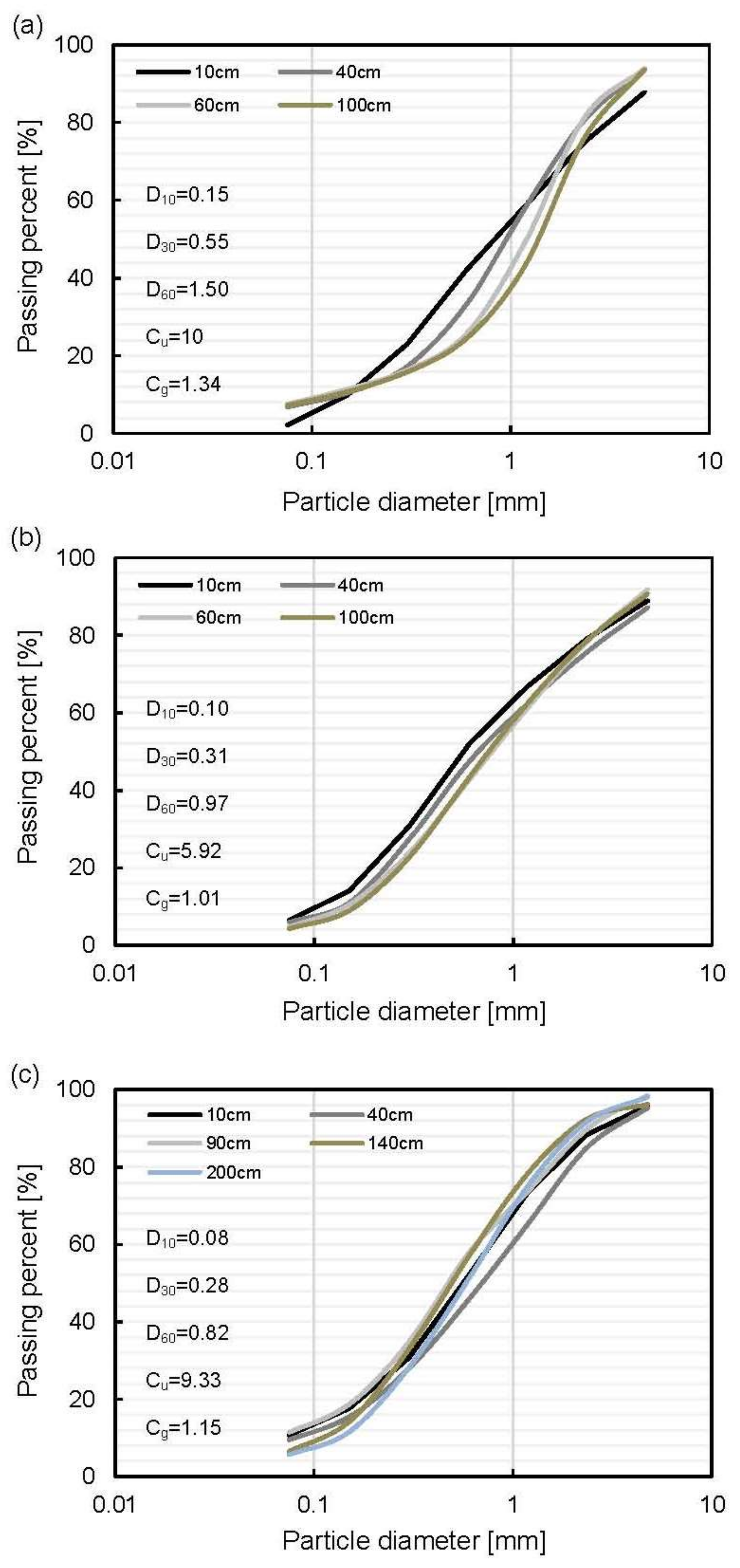
A hand auger with an outer diameter of 20 cm was used to excavate the subsurface and a soil sampler was used to gather the specimen at the wall of a borehole. The length of the hand auger was limited to 2 m due to a shortage of engine output, and thus the maximum depth of extracted soil in this study was 2 m. Even though the hand auger can potentially excavate soil down to a maximum of 2 m, the actual excavated depth was reduced due to the presence of gravel and weathered rock. Therefore, the actual maximum extracted depths were 1, 1, and 2 m at locations near points A, B, and C, respectively. The results from the excavations at points A and B show various deposited materials, including gravel and boulder (Figure 2). At point C near the initial zone, a larger extraction depth (~2 m) could be achieved due to the presence of a relatively deep soil layer (Figure 2). Soil samples were collected at 4–5 different depths: 10, 40, 60, and 100 cm for points A and B; and 10, 40, 90, 140, and 200 cm for point C. Sieve tests were performed using the extracted specimens according to [15].
The results of sieve tests are shown in Figure 2. The diameters at passing percentages of 10, 30 and 60% are calculated for every specimen, to classify the specimen based on the unified soil classification system. The calculated coefficients of uniformity are 10, 5.92, and 9.33 for extracted soils at points A, B, and C, respectively. The coefficients of curvature at points A, B, and C are determined to be 1.34, 1.01, and 1.51, respectively. The measured coefficients of uniformity show values almost greater than 6 and the coefficients of curvature are in the range of 1~3; hence, the specimens at testing sites are classified as SW (well-graded sand). Additionally, Figure 2 indicates that the grain size distributions of extracted samples at different depths are very similar.
3. Methodology
A seismic survey and dynamic cone penetrometer test were performed to obtain primary wave velocity and dynamic cone penetration index (DPI), respectively, and the detailed descriptions are as follows.
3.1. Seismic Survey
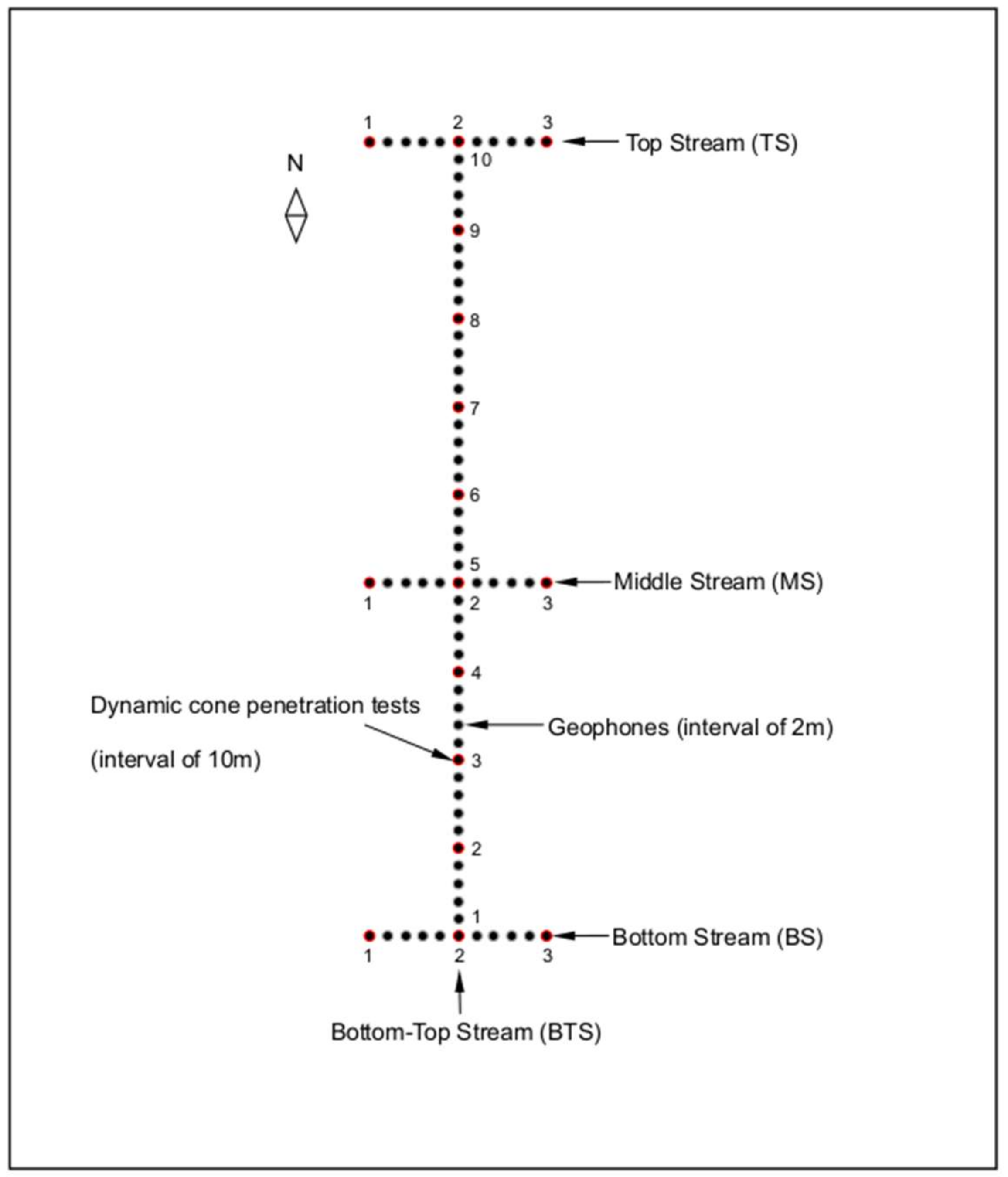
A seismic survey has the advantage of assessing a whole area without altering the fabric state; thus, the measured values can greatly reflect the state and behavior of soils. A seismic wave propagates in solid media by travelling through particle connections, and thus the wave velocity increases with an increase in the particle contact area (or applied confining stress or soil depth). The seismic refraction method was applied in this study to obtain a profile of compressional (or primary) wave velocity. Four transects were determined with consideration for spatial variability in the geological characterization of each stream. Figure 3 shows schematic drawings of the seismic transections. The bottom-top stream (BTS) line reflects the main stream from south to north (from points A to D in Figure 1), whereas the bottom stream (BS), middle stream (MS), and top stream (TS) lines are horizontally set to reflect bottom, middle, and top valleys, respectively. The center of the MS line is located between points B and C in Figure 1. The lengths of the transection lines are 90, 20, 20, and 20 m for BTS, BS, MS, and TS, respectively. A geophone was installed as a sensor for gathering seismic waves every 2 m; therefore, the installed geophone numbers in the profiles of BTS, BS, MS and TS are 45, 10, 10, and 10, respectively. A sledgehammer was used to generate vibrations, and the impactions were performed at start, middle, and end positions to enhance signal-to-noise ratios. Impactions were performed five times in the same position for each test to minimize random noise.
3.2. Dynamic Cone Penetrometer Test
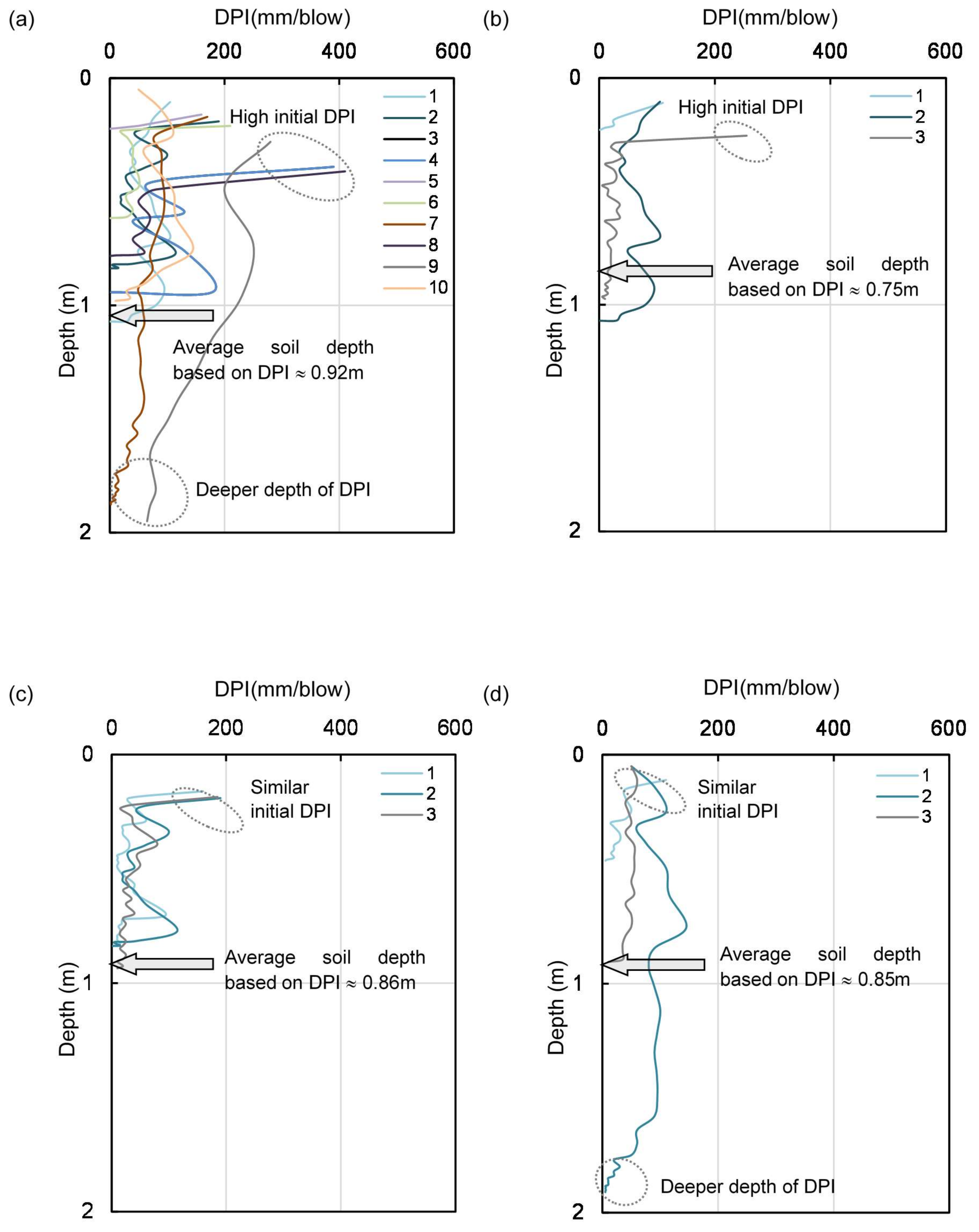
A dynamic cone penetrometer (DCP) test was selected as an invasive method to verify the soil depths estimated by seismic waves. Note that the DCP method can readily detect the thickness of soil layer because the continuous penetration of DCP enables the easy recognition of the presence of different layers [16]: the penetration depth through stiff material is relatively small. The DCP technique has been widely applied to investigate soil properties in geotechnical engineering, especially for railways and roads [16,17,18]. The test records the penetration depth of DCP when a hammer drops from a fixed height according to [19]. The hammer weight and drop height were fixed to 78.8 N and 575 mm, respectively. The tip diameter of the DCP was 20 mm with an apex angle of 60°, and driving energy was 45 J. The penetration depth was converted into dynamic penetration index (DPI), which represents (mm/blow) as follows.
where P = penetration depth (mm); B = blow count; and i and i + 1 = experimental number.
4. Results and Analysis
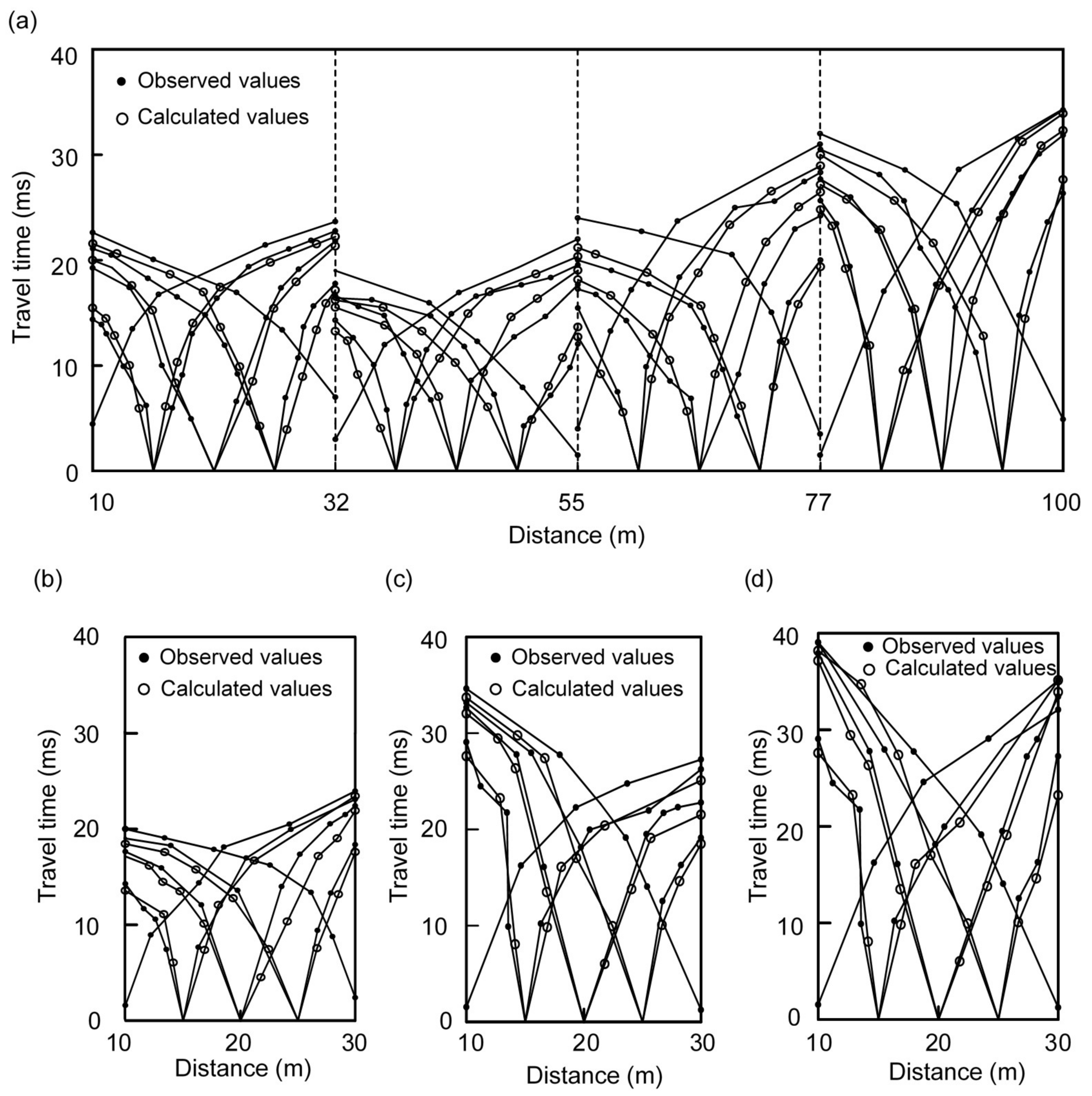
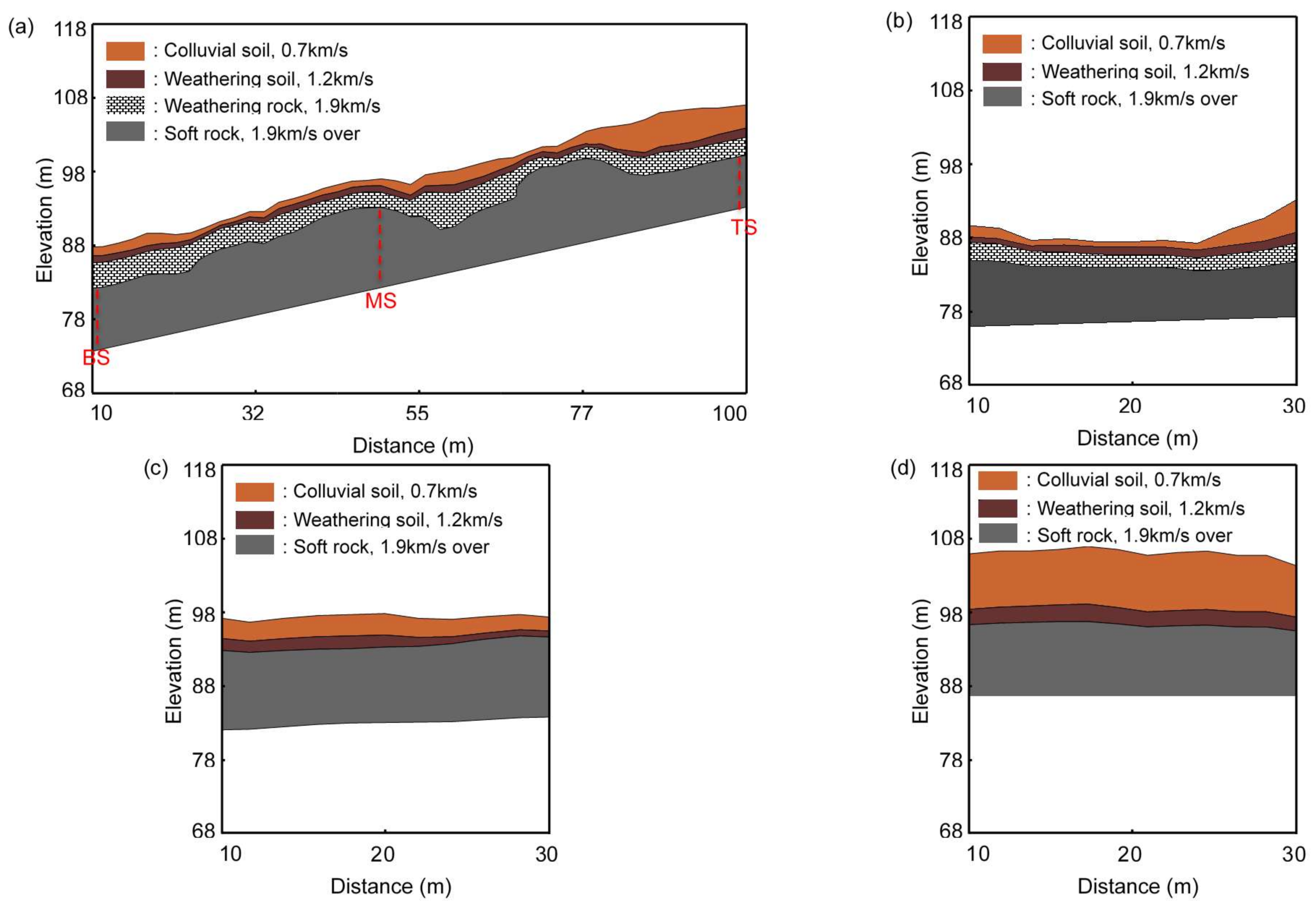
The first arrival time of the measured seismic wave signals was determined through PickWin software (OYO corporation, Tokyo, Japan), and the time-distance curve was obtained by using the SeisImager-Poltrefa program (OYO corporation, Tokyo, Japan). An interactive process was performed to increase resolution when carrying out the inversion process. Two groups, which are based on the picked first-arrival times and the results analyzed by the simultaneous iterative method, are plotted on a travel-time curve in Figure 4. Figure 4 shows that the two groups are nearly identical, reflecting that the quality of the measured data is high. The distribution of seismic wave velocity is plotted in Figure 5, and the soil layers are divided into various different layers according to the reference P-wave velocities suggested by [20]: 0–0.7 km/s (landfill and alluvial soil), 0.7–1.2 km/s(weathered soil), 1.2–1.9 km/s (weathered rock), and over 1.9 km/s (soft rock). The BTS, BS, MS, and TS lines were found to comprise four, four, three, and three layers, respectively based on Reynolds (2003). Note that 0.7 km/s of primary wave velocity is an accepted criterion in South Korea for distinguishing soil layers from other geomaterials [21,22].
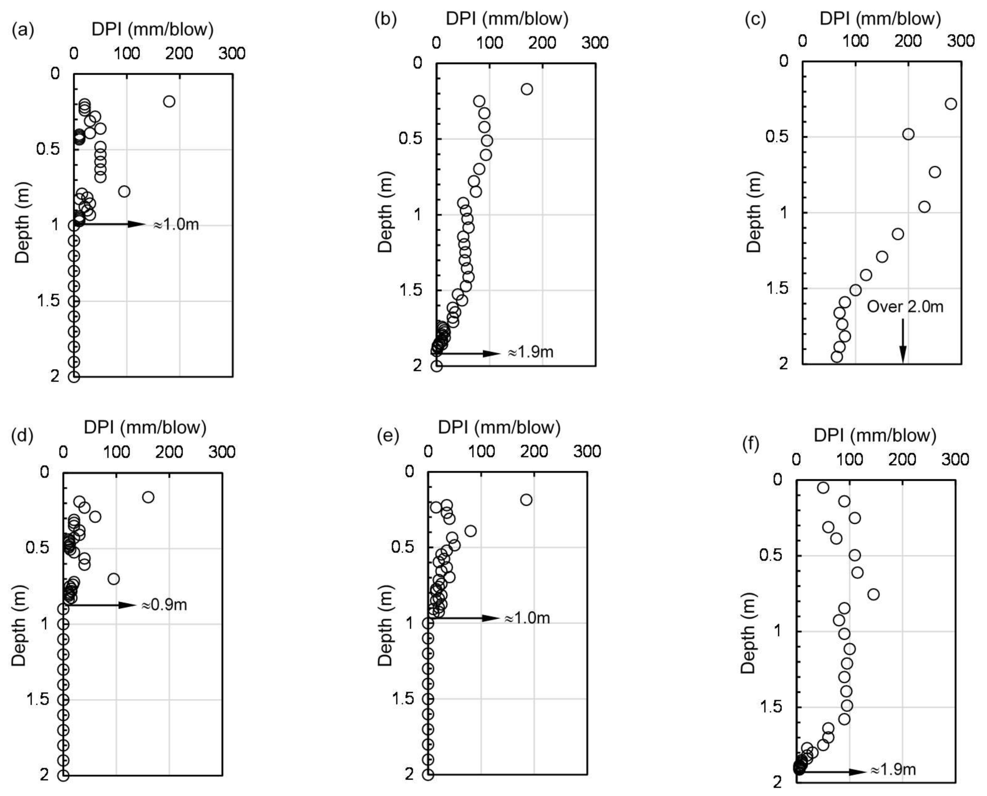
The calculated DPI values from dynamic cone penetration tests are shown in Figure 6 for each stream. The BTS line shows high variation of DPI values according to the testing locations, which are described in Figure 3, because the line covers the bottom, middle, and top streams. Note that the high variation of DPI values means that the soil depth changes along the stream in the BTS line. Number 4, 8 and 9 holes in Figure 6a show high DPI values at shallow depth, reflecting the presence of weak soil layers. Being different from other testing holes, the DPI was measured at deeper depths at No. 7 and 9 holes, demonstrating that the soil depth near the top stream is deeper than that of other locations. Note that Figure 5a and the maximum extracted soil depth using a hand auger also support the presence of deep soil layer near the top stream in the BTS line. In the case of the BS line, high DPI values at the initial stage and high penetrated depth were observed at the right side of the stream. A similar DPI trend was observed in the MS line, and the distributions of soil depth in the No. 1, 2, and 3 holes look alike, reflecting similar soil depths along the MS line. Even though the DPI of the TS line shows a similar penetrated depth near the surface, the DPI was continuously measured at the only No. 2 hole. Therefore, it is predicted that the soil depth at the No. 2 hole, which is the center of the TS line, is high. The depth where the DPI value is close to zero is referred to as the soil depth of the testing site in this study, and the average soil depths based on DPI are calculated to be approximately 0.92, 0.75, 0.86 and 0.85 m for the BTS, BS, MS, and TS lines, respectively.
Comparison between Figure 5 and Figure 6 reveals that the soil depth of the testing site based on dynamic cone penetration test is generally shallower than 1 m; while, the depth based on seismic wave velocity (0.7 km/s) is around 2 m or more (Table 1), reflecting that the subsurface classification based on previous reference values of seismic wave velocity cannot precisely estimate the soil depth. Therefore, in this study, the graphical bilinear method is newly suggested for determining soil depth based on seismic wave velocity.
5. Discussion
The seismic refraction method measures the travel time of the waves refracted at the interface between different sublayers with different wave velocities or impedances. Thus, the thickness of each layer can be calculated using the wave velocities of two consecutive layers and the time intercept in the travel time-distance curve as:
where Z = thickness of layer; t = time intercept; V = wave velocity; and i and i + 1 = different layers. The thickness of the soil layer (or the first layer) can be determined by the velocities of the first layer and the second layer (V1 and V2), and the time intercept (t1). However, the clear determination of V1, V2, and t1 is not easy because wave velocity in a given layer is not constant, resulting from the natural soil deposits rarely being homogeneous and wave velocity slightly increasing with an increase in depth at a given layer. Note that seismic waves propagate in a medium through connected particles, and seismic wave velocity depends on soil structure and stress condition. Seismic wave propagation is primarily affected by the stiffness of the fabric in a particular material, and thus seismic wave velocity and effective stress (σ′) have a certain relationship with experimentally determined coefficients (α and β).
The α and β coefficients are dependent on the packing type (porosity and coordination number) and the contact force (Hertzian contact and Coulombic force).
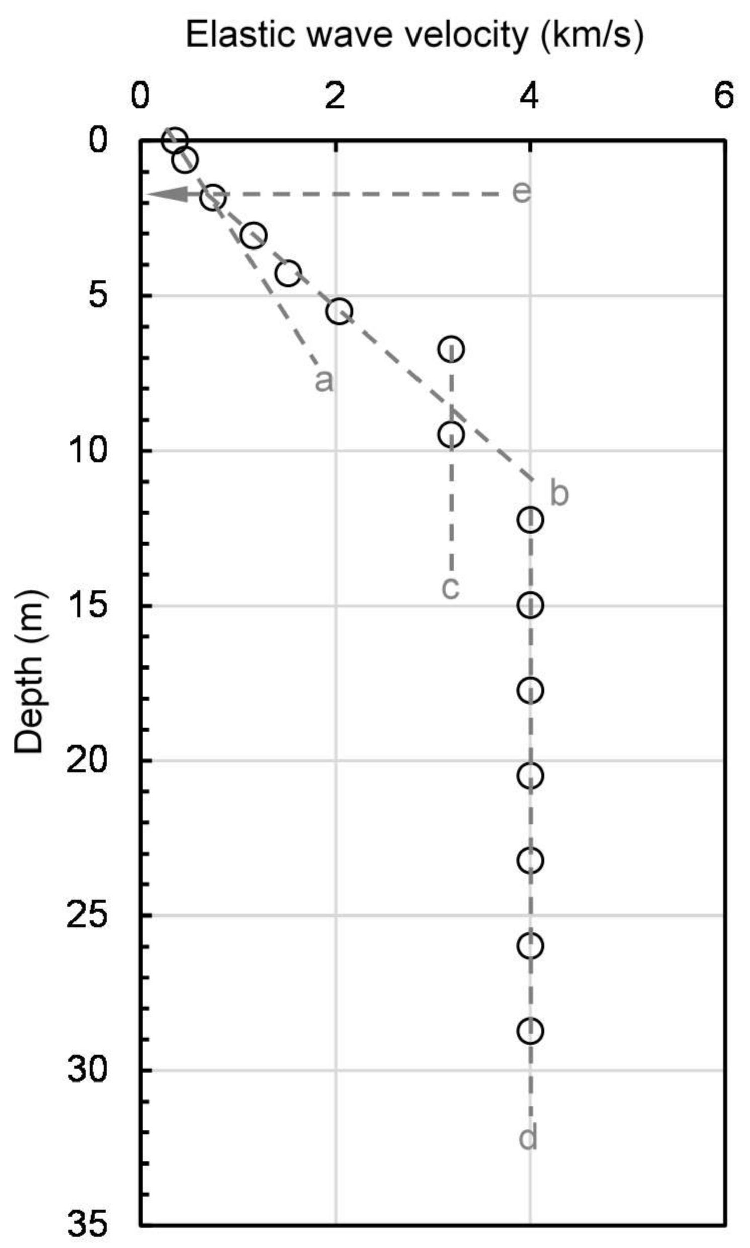
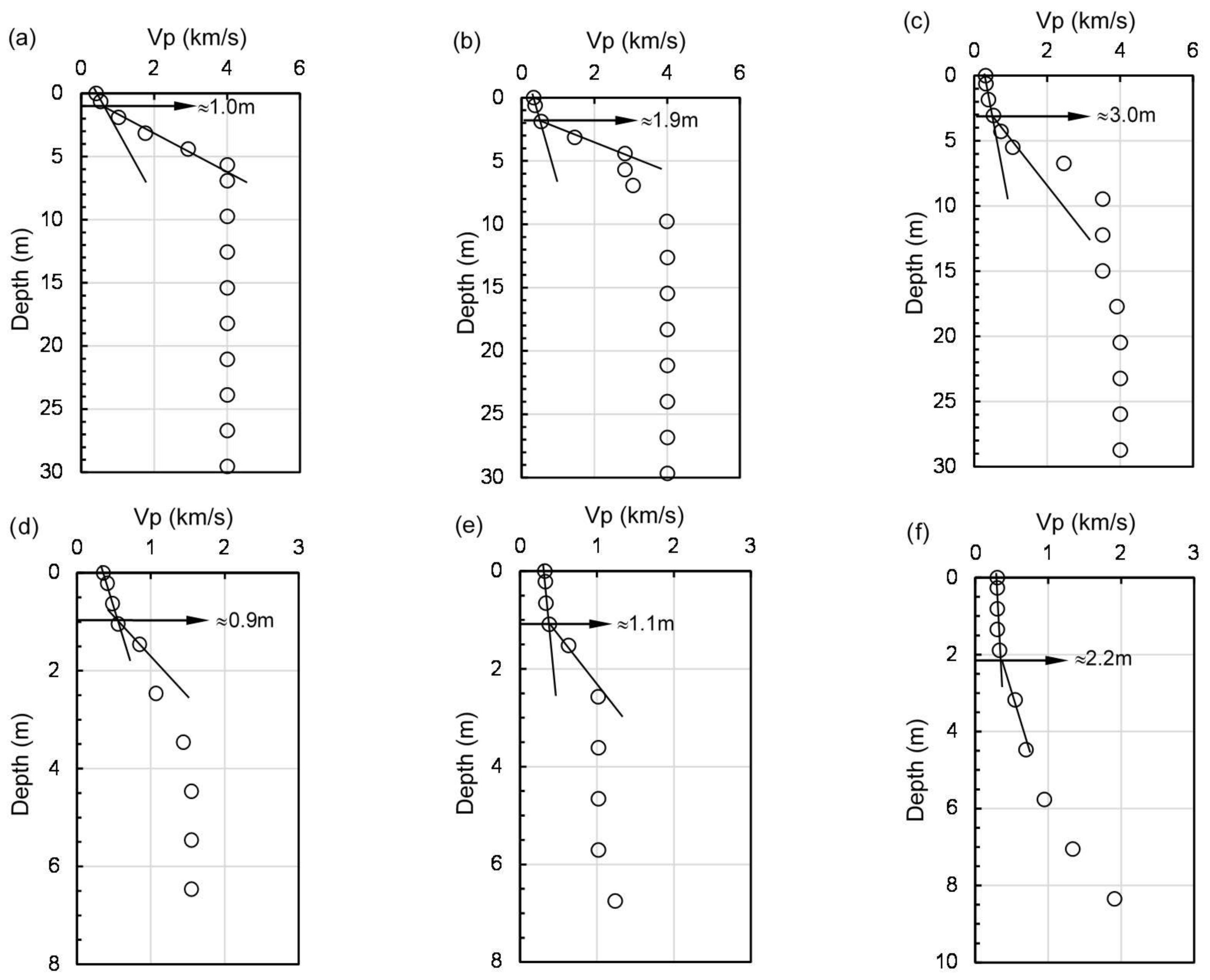
The seismic wave velocity slightly increases with depth even in one layer because of the increase in effective stress (Equation (3)), which is the function of mass density and depth. However, the wave velocity changes rapidly at layer boundaries due to the change in material type, mass density, particle size, and others. Hence, the relation between seismic wave velocity and depth can produce different slopes along the depth. Figure 7 shows the seismic wave velocity with the depth at which the geophones are installed. It can be observed in Figure 7 that there are four different lines “a”, “b”, “c”, and “d”: Line “a” indicates the initial slope between wave velocity and depth; thus, it is related to the first soil layer; Line “b” indicates the second slope between wave velocity and depth; thus, it is related to the second layer. Therefore, the intersection point between lines “a” and “b” may correspond to the thickness of the first soil layer, which is point “e”. Figure 8 shows the calculated soil depths based on the suggested graphical bilinear method at the selected testing sites. It is shown in Figure 8 that various soil depths can be estimated by the proposed method. The detailed soil depths based on the suggested graphical bilinear method are summarized in Table 1.
The measured DPI values at the selected testing sites are plotted in Figure 9 to determine soil depth based on the impaction study. Soil depth is estimated to the maximum penetrated depth at which the DPI value is nearly zero. Even though the DPI shows variation with depth within a borehole, the final penetrated depth can be easily calculated based on the depth where the value of DPI is close to zero. Figure 9c shows that DPI does not converge close to zero until a depth of 2 m. The maximum possible experiment depth is fixed to 2 m due to the rod length and energy transfer during impaction, thus the soil depth is expected to be greater than 2 m. This deeper expected soil depth can be anticipated because the soil thickness was estimated to be approximately 3.0 m based on the graphical bilinear method shown in Figure 8c for the same position as in Figure 9c. Table 1 summarizes the soil depth calculated by dynamic cone penetration tests.
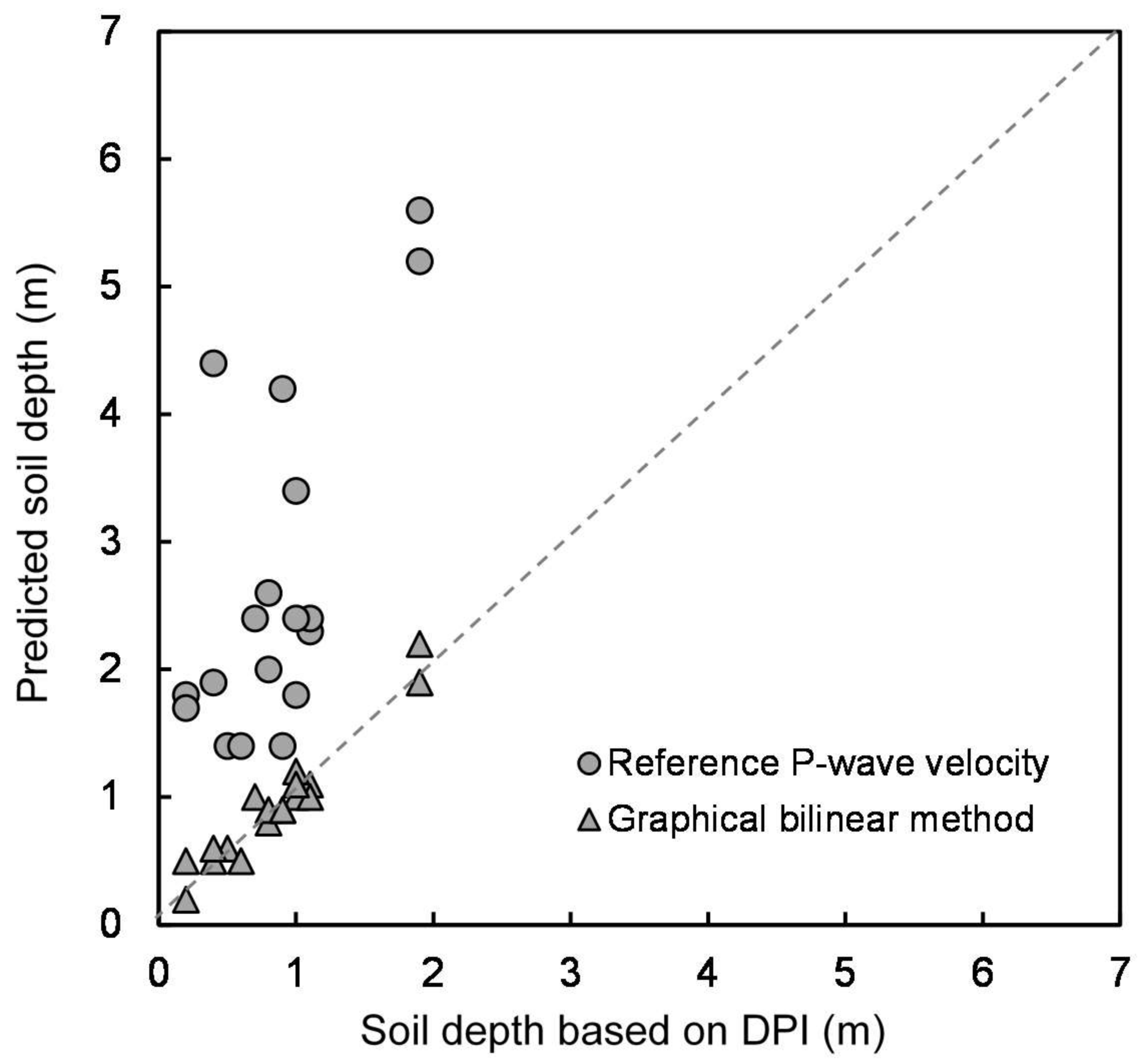
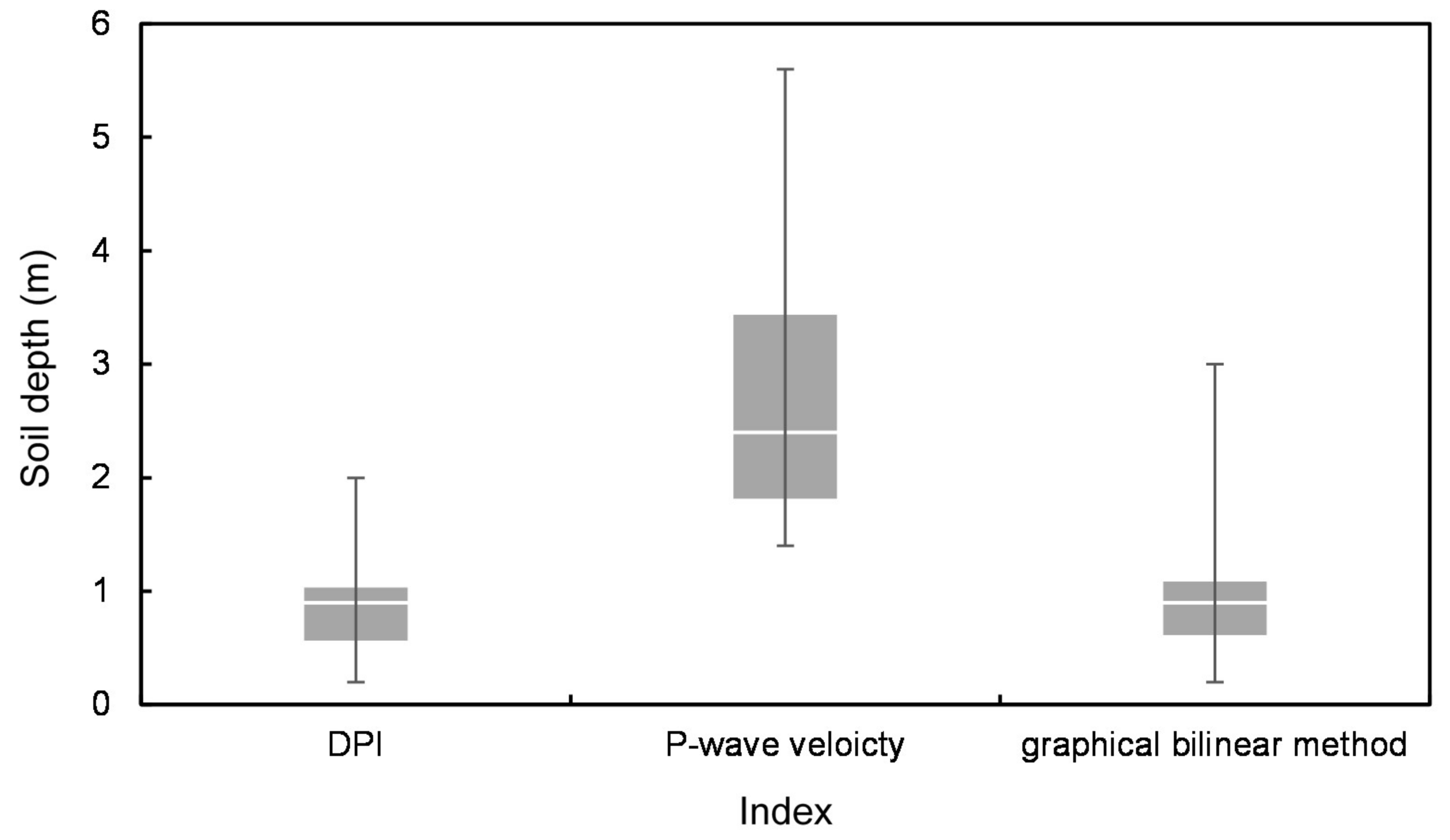
Figure 10 shows the comparison of soil depths predicted by the reference P-wave velocity (0.7 km/s) and the graphical bilinear method with the measured depths using dynamic cone penetration test. Note that the depth based on the results of the dynamic cone penetration test (DPI values) has relatively high reliability because the data is gathered through direct penetration of the probe into soil; therefore, the soil depth measured by DPI can be regarded as the real soil depth. The soil depth predicted based on the reference P-wave velocity shows high variation and high soil depth compared with those based on DPI values. In contrast, the soil depth based on the graphical bilinear method shows small variation and the estimated values are comparable with the measured values by dynamic cone test, reflecting the enhanced reliability of the estimated soil depth by using the suggested method. Furthermore, the deduced soil depths based on DPI, P-wave velocity and graphical bilinear method are compared through box and whisker plot as shown in Figure 11. The median values of DPI and graphical bilinear method show 0.35 m and 0.3 m, and however the median soil depth based on P-wave velocity is highly deduced to 0.5 m. The first and third quartiles of DPI and graphical bilinear method show also similar ranges of 0.15–0.55 m and 0.2–0.6 m, respectively and it shows the difference is just 0.5 m. However, the soil depth estimated by existing method shows unreasonable ranges of 1.05–1.8 m. The ranges of minimum and maximum values based on DPI (0.2–2 m) and suggested method (0.2–3 m) are also demonstrated to similar trends while those deduced by P-wave velocity exhibited huge variations (1.4–5.6 m). And thus, the Figure 11 shows that the suggested method can provide the reliable soil depth under ≈3 m with consideration of 2 m intervals of geophone.
Table 1 shows the calculated error ratios (error ratio = (estimated value − measured value)/measured value). The estimated soil depths based on reference P-wave velocity show high error ratios, ranging from 55% to 1000%, and the average value shows approximately over 100%, reflecting the estimation of soil depth using the classification of soil layers based on reference wave velocity is not reliable. In contrast, the graphical bilinear method shows relatively small average error ratios of 28.2, 6.6, 10.5, and 21.9% for BTS, BS, MS, and TS, respectively, demonstrating that the graphical bilinear method suggested in this study provides reliable estimation of soil depth.
6. Conclusions
This paper suggests methods for the determination of soil depth through seismic wave velocity measurements. The graphical bilinear method is newly introduced, and the soil depth estimated with the suggested method is compared with the result of dynamic cone penetration tests. The results of this study demonstrate the following:
- The estimated soil depth using the soil classification based on the reference P-wave velocity shows high variation and high soil depth compared with that based on dynamic cone penetration test, reflecting the estimation of soil depth based on the reference wave velocity is not reliable.
- The seismic wave velocity slightly increases with depth even in one layer and it changes rapidly at layer boundaries. Because the graphical bilinear method newly suggested in this study is based on the change in the slope between wave velocity and depth, the estimated soil depths using the suggested method are comparable with the measured values by dynamic cone test, reflecting the enhanced reliability in estimating soil depth by seismic survey.
Acknowledgments
This work was supported by the National Research Foundation of Korea (NRF) grant funded by the Korea government (MSIP) (NRF-2017R1A2B4008157).
Author Contributions
Hyunwook Choo, Hwandon Jun and Hyung-Koo Yoon performed field experiments and wrote paper together.
Conflicts of Interest
The authors declare no conflict of interest.
References
- Kamatchi, P.; Rajasankar, J.; Iyer, N.R.; Lakshmanan, N.; Ramana, G.V.; Nagpal, A.K. Effect of depth of soil stratum on performance of buildings for site-specific earthquakes. Soil Dyn. Earthq. Eng. 2010, 30, 647–661. [Google Scholar] [CrossRef]
- Francés, A.P.; Lubczynski, M.W. Topsoil thickness prediction at the catchment scale by integration of invasive sampling, surface geophysics, remote sensing and statistical modeling. J. Hydrol. 2011, 405, 31–47. [Google Scholar] [CrossRef]
- Ho, J.Y.; Lee, K.T.; Chang, T.C.; Wang, Z.Y.; Liao, Y.H. Influences of spatial distribution of soil thickness on shallow landslide prediction. Eng. Geol. 2012, 124, 38–46. [Google Scholar] [CrossRef]
- Adhikary, S.; Singh, Y.; Paul, D.K. Effect of soil depth on inelastic seismic response of structures. Soil Dyn. Earthq. Eng. 2014, 61, 13–28. [Google Scholar] [CrossRef]
- Bao, X.; Liao, W.; Dong, Z.; Wang, S.; Tang, W. Development of Vegetation-Pervious Concrete in Grid Beam System for Soil Slope Protection. Materials 2017, 10, 96. [Google Scholar] [CrossRef] [PubMed]
- Han, Z.; Wang, Y.; Qing, X. Characteristics Study of In-Situ Capacitive Sensor for Monitoring Lubrication Oil Debris. Sensors 2017, 17, 2851. [Google Scholar] [CrossRef] [PubMed]
- Heimsath, A.M.; Dietrich, W.E.; Nishiizumi, K.; Finkel, R.C. Cosmogenic nuclides, topography, and the spatial variation of soil depth. Geomorphology 1999, 27, 151–172. [Google Scholar] [CrossRef]
- Kuriakose, S.L.; Devkota, S.; Rossiter, D.G.; Jetten, V.G. Prediction of soil depth using environmental variables in an anthropogenic landscape, a case study in the Western Ghats of Kerala, India. Catena 2009, 79, 27–38. [Google Scholar] [CrossRef]
- Trustrum, N.A.; De Rose, R.C. Soil depth-age relationship of landslides on deforested hillslopes, Taranaki, New Zealand. Geomorphology 1988, 1, 143–160. [Google Scholar] [CrossRef]
- Kirkby, M.J. A model for the evolution of regolith-mantled slopes. In Models Geomorphology; Allen and Unwin: London, UK, 1985; pp. 213–237. [Google Scholar]
- Dietrich, W.E.; Reiss, R.; Hsu, M.L.; Montgomery, D.R. A process-based model for colluvial soil depth and shallow landsliding using digital elevation data. Hydrol. Process. 1995, 9, 383–400. [Google Scholar] [CrossRef]
- Gallipoli, M.; Lapenna, V.; Lorenzo, P.; Mucciarelli, M.; Perrone, A.; Piscitelli, S.; Sdao, F. Comparison of geological and geophysical prospecting techniques in the study of a landslide in southern Italy. Eur. J. Environ. Eng. Geophys. 2000, 4, 117–128. [Google Scholar]
- De Vita, P.; Agrello, D.; Ambrosino, F. Landslide susceptibility assessment in ash-fall pyroclastic deposits surrounding Mount Somma-Vesuvius: Application of geophysical surveys for soil thickness mapping. J. Appl. Geophys. 2006, 59, 126–139. [Google Scholar] [CrossRef]
- Min, D.H.; Park, C.H.; Lee, J.S.; Yoon, H.K. Estimating Soil Thickness in a Debris Flow using Elastic Wave Velocity. J. Eng. Geol. 2016, 26, 143–152. [Google Scholar] [CrossRef]
- Standard Test Method for Sieve Analysis of Fine and Coarse Aggregates; ASTM, C136; ASTM: West Conshohocken, PA, USA, 1984.
- Mohammadi, S.D.; Nikoudel, M.R.; Rahimi, H.; Khamehchiyan, M. Application of the Dynamic Cone Penetrometer (DCP) for determination of the engineering parameters of sandy soils. Eng. Geol. 2008, 101, 195–203. [Google Scholar] [CrossRef]
- Brough, M.; Stirling, A.; Ghataora, G.; Madelin, K. Evaluation of railway trackbed and formation: A case study. NDT & E Int. 2003, 36, 145–156. [Google Scholar]
- Salgado, R.; Yoon, S. Dynamic cone penetration test (DCPT) for subgrade assessment. Jt. Transp. Res. Program 2003, 73, 20–28. [Google Scholar]
- Standard Test Method for Use of the Dynamic Cone Penetrometer in Shallow Pavement Applications; ASTM D6951/D6951M-09; ASTM: West Conshohocken, PA, USA, 2015.
- Reynolds, J.M. An Introduction to Applied and Environmental Geophysics; Wiley: New York, NY, USA, 2003. [Google Scholar]
- Lee, K.M.; Kim, H.; Lee, J.H.; Seo, Y.S.; Kim, J.S. Analysis on the Influence of Groundwater Level Changes on Slope Stability using a Seismic Refraction Survey in a Landslide Area. J. Eng. Geol. 2007, 17, 545–554. [Google Scholar]
- Hong, W.P.; Kim, J.H.; Ro, B.D.; Jeong, G.C. Case Study on Application of Geophysical Survey in the Weathered Slope including Core Stones. J. Eng. Geol. 2009, 19, 89–98. [Google Scholar]
Figure 1.
Aerial photography of the testing area. Points A and D denote the bottom and top streams, respectively. Points B and C indicate the middle stream. The field tests were performed from points A to D.
Figure 1.
Aerial photography of the testing area. Points A and D denote the bottom and top streams, respectively. Points B and C indicate the middle stream. The field tests were performed from points A to D.

Figure 2.
Sieve test results: (a) bottom stream (point A in Figure 1); (b) middle stream (point B); (c) top stream (point C). D10, D30, and D60 denote the diameters at passing percentages of 10, 30, and 60%, respectively. Cu and Cg are coefficients of uniformity and curvature, respectively.
Figure 2.
Sieve test results: (a) bottom stream (point A in Figure 1); (b) middle stream (point B); (c) top stream (point C). D10, D30, and D60 denote the diameters at passing percentages of 10, 30, and 60%, respectively. Cu and Cg are coefficients of uniformity and curvature, respectively.

Figure 3.
Locations of the field investigations, including seismic survey and dynamic cone penetrometer (DCP). Note: the numbers with red circles denote the DCP testing sites (BS: 3 holes, MS: 3 holes, TS: 3 holes, and BTS: 10 holes); and the distance between each number in the figure is 10 m.
Figure 3.
Locations of the field investigations, including seismic survey and dynamic cone penetrometer (DCP). Note: the numbers with red circles denote the DCP testing sites (BS: 3 holes, MS: 3 holes, TS: 3 holes, and BTS: 10 holes); and the distance between each number in the figure is 10 m.

Figure 4.
Travel time-distance curves through seismic survey: (a) BTS; (b) BS; (c) MS; and (d) TS. Note 10, 20, 30, and 100 m distances indicate points 1, 2, 3, and 10, respectively, in Figure 3.
Figure 4.
Travel time-distance curves through seismic survey: (a) BTS; (b) BS; (c) MS; and (d) TS. Note 10, 20, 30, and 100 m distances indicate points 1, 2, 3, and 10, respectively, in Figure 3.

Figure 5.
Converted primary wave velocity profiles: (a) BTS; (b) BS; (c) MS; and (d) TS.

Figure 6.
Measured DPI values of each stream: (a) BTS; (b) BS; (c) MS; and (d) TS. Note the numbers in each figure indicate the location of dynamic cone penetration test described in Figure 3.
Figure 6.
Measured DPI values of each stream: (a) BTS; (b) BS; (c) MS; and (d) TS. Note the numbers in each figure indicate the location of dynamic cone penetration test described in Figure 3.

Figure 7.
Method for selecting soil depth through measured elastic wave velocity. Line “a” denotes the first slope between wave velocity and depth. Lines “b”, “c”, and “d” represent the second, third and fourth slopes, respectively. Point “e” is the intersection point between lines “a” and “b”. Note the figure is the relation between wave velocity and depth of point 1 (or 10 m distance) in the BTS line (Figure 3).

Figure 8.
Estimated soil depth profile based on graphical bilinear method: (a) 30 m of BTS; (b) 80 m of BTS; (c) 100 m of BTS; (d) 20 m of BS; (e) 30 m of MS; and (f) 20 m of TS.
Figure 8.
Estimated soil depth profile based on graphical bilinear method: (a) 30 m of BTS; (b) 80 m of BTS; (c) 100 m of BTS; (d) 20 m of BS; (e) 30 m of MS; and (f) 20 m of TS.

Figure 9.
Soil depth based on dynamic cone penetration test: (a) 30 m of BTS; (b) 80 m of BTS; (c) 100 m of BTS; (d) 20 m of BS; (e) 30 m of MS; and (f) 20 m of TS.
Figure 9.
Soil depth based on dynamic cone penetration test: (a) 30 m of BTS; (b) 80 m of BTS; (c) 100 m of BTS; (d) 20 m of BS; (e) 30 m of MS; and (f) 20 m of TS.

Figure 10.
Comparison of soil depths estimated by seismic wave velocity and measured by dynamic cone penetration test.
Figure 10.
Comparison of soil depths estimated by seismic wave velocity and measured by dynamic cone penetration test.

Figure 11.
Comparison of soil depths through box plot.


Table 1.
Comparison between Measured and Estimated Soil Depths.
| Position | Soil Depth (m) | Error Ratio (%) | ||||
|---|---|---|---|---|---|---|
| Measured | Estimated | |||||
| Dynamic Cone Test | Reference P-Wave Velocity | Graphical Bilinear Method | Reference P-Wave Velocity | Graphical Bilinear Method | ||
| BTS | 1 | 1.1 | 2.3 | 1.1 | 109.1 | 0.0 |
| 2 | 0.8 | 2.0 | 0.8 | 150.0 | 0.0 | |
| 3 | 1.0 | 1.8 | 1.0 | 80.0 | 0.0 | |
| 4 | 0.4 | 1.9 | 0.5 | 375.0 | 25.0 | |
| 5 | 0.5 | 1.4 | 0.6 | 180.0 | 20.0 | |
| 6 | 0.2 | 1.8 | 0.5 | 800.0 | 150.0 | |
| 7 | 0.6 | 1.4 | 0.5 | 133.3 | 16.7 | |
| 8 | 0.7 | 2.4 | 1.0 | 242.9 | 42.9 | |
| 9 | 1.9 | 5.6 | 1.9 | 194.7 | 0.0 | |
| 10 | Over 2.0 | 3.5 | 3.0 | - | - | |
| Average | 251.7 | 28.2 | ||||
| BS | 1 | 0.2 | 1.7 | 0.2 | 750.0 | 0.0 |
| 2 | 0.9 | 1.4 | 0.9 | 55.6 | 0.0 | |
| 3 | 1.0 | 3.4 | 1.2 | 240.0 | 20.0 | |
| Average | 348.5 | 6.6 | ||||
| MS | 1 | 1.1 | 2.4 | 1.0 | 118.2 | 9.1 |
| 2 | 0.8 | 2.6 | 0.9 | 225.0 | 12.5 | |
| 3 | 1.0 | 2.4 | 1.1 | 140.0 | 10.0 | |
| Average | 161.1 | 10.5 | ||||
| TS | 1 | 0.4 | 4.4 | 0.6 | 1000.0 | 50.0 |
| 2 | 1.9 | 5.2 | 2.2 | 173.7 | 15.8 | |
| 3 | 0.9 | 4.2 | 0.9 | 366.7 | 0.0 | |
| Average | 513.5 | 21.9 | ||||
Note: error ratio = (estimated value − measured value)/measured value; the numbers in Position column indicate the testing locations in Figure 3.
© 2018 by the authors. Licensee MDPI, Basel, Switzerland. This article is an open access article distributed under the terms and conditions of the Creative Commons Attribution (CC BY) license (http://creativecommons.org/licenses/by/4.0/).
Share and Cite
MDPI and ACS Style
Choo, H.; Jun, H.; Yoon, H.-K. Application of Elastic Wave Velocity for Estimation of Soil Depth. Appl. Sci. 2018, 8, 600. https://doi.org/10.3390/app8040600
AMA Style
Choo H, Jun H, Yoon H-K. Application of Elastic Wave Velocity for Estimation of Soil Depth. Applied Sciences. 2018; 8(4):600. https://doi.org/10.3390/app8040600
Chicago/Turabian StyleChoo, Hyunwook, Hwandon Jun, and Hyung-Koo Yoon. 2018. "Application of Elastic Wave Velocity for Estimation of Soil Depth" Applied Sciences 8, no. 4: 600. https://doi.org/10.3390/app8040600
Note that from the first issue of 2016, this journal uses article numbers instead of page numbers. See further details here.