Adaptive Trajectory Tracking Control for Underactuated Unmanned Surface Vehicle Subject to Unknown Dynamics and Time-Varing Disturbances

Abstract

This paper proposes an adaptive trajectory tracking control strategy for underactuated unmanned surface vehicles subject to unknown dynamics and time-varing external disturbances. In short, the goal of this paper is to provide a control strategy that allows an underactuated unmanned surface vehicle to track a time dependent trajectory. First, a first-order sliding surface is introduced into the design of surge control law to converge to surge tracking error, and then a second-order sliding surface is hired to design yaw control law to deal with sway motion tracking error. Meanwhile, neural network minimum learning parameter method, which has a smaller amount of computation than a multilayer neural network, is employed to preserve the control law robustness against unknown dynamics and time-varing disturbances induced by wind, waves and ocean currents. Furthermore, much effort is made to obtain uniform ultimate bounded stability for the closed-loop control system. Finally, the numerical simulation experiments of straight line and circle trajectory tracking have been given to prove the correctness and feasibility of the proposed control strategy.

1. Introduction

With the continuous advancement of science and technology, the modern ship system is moving toward a systematic, intelligent and unmanned direction. In recent years, a new type of ship research project has been developed by combining the achievements of small speedboats and advanced control technologies, like the Unmanned Surface Vehicles (USVs) [1,2]. Following the trend of ship systems, USVs has become a unique research field, which attracts more and more institutions and researchers to conduct relevant research [3,4]. Generally, trajectory tracking is an important topic in the field of USV research, and it is the guarantee for many applications in the future, such as formation operations, and so on [5,6]. However, a very realistic and urgent problem to be solved is that the overwhelming majority of USVs with propellers and rudders belong to an underactuated system, while without any actuators for direct control of sway motion [7,8,9]. Therefore, how to design robust trajectory tracking controllers under the condition of underactuated characteristics for USVs is a very worthwhile problem.

Many researchers have made outstanding contributions to cope with the trajectory tracking problem for underactuated ships [10,11,12,13]. In [14], a unified backstepping design methodology is hired to solve the stabilisation and tracking problems for an underactuated ship with only two propellers. Chwa proposes a modular way that cascaded kinematic and dynamic linearizations can be achieved similarly as in the backstepping method. Based on this, under the premise of input and velocity constraints, dynamic surface control (DSC) technology is used to design a trajectory tracking control strategy for an underactuated ship [15]. For an underactuated USV, the experimental implementation of two trajectory tracking control algorithms: a cascade of proportional-derivative controllers and a nonlinear controller are proposed by Sonnenburg et al. through the backstepping control technology [16]. In [17,18], for an underactuated USV, the switching control and modified backstepping methods are used to design the trajectory tracking controller, which can track a straight line track or fixed point. However, in actual navigation, besides the external disturbances caused by wind, waves and currents, the ship’s quality, speed and moment of inertia will also change, which will lead to some changes or unknown dynamics in the model of ship. In [19], the backstepping method is hired to design the USV trajectory tracking controller. At the same time, a disturbance observer is employed to compensate for the time-varying external disturbances on line. The sliding mode algorithms have strong robustness, which are often introduced into the motion control of various nonlinear systems. Hierarchical sliding mode-based trajectory tracking controller is designed to allow the underactuated surface vessels to track a pre-specified trajectory [20]. Besides, in [21], the sliding mode control algorithm is introduced into the design of a trajectory tracking controller for underactuated USV, but it does not consider the effects of unknown dynamics and time-varing disturbances. In practical engineering application, when dealing with model structure unknown or unknown dynamics problems, the universal approximation ability of neural network [22,23] or fuzzy logic [24,25,26] is widely used. Fuzzy logic needs experts’ prior knowledge, which often increases the design difficulty of controller. So the multilayer neural network represented by radial basis function (RBF) neural network is the most widely used method to deal with the unknown dynamics problem. Paper [27] proposes a single layer neural network to cope with the completely unknown vehicle dynamics for an autonomous surface vehicle (ASV) to track a predetermined trajectory.

Motivated by the above-mentioned observations, an adaptive trajectory tracking control strategy for engineering implementation, which is performed by using first-order sliding surface, second-order sliding surface and neural network minimum learning parameter method, is designed for an underactuated USV subject to unknown dynamics and time-varing external disturbances. The contributions of this paper can be summarized as follows:

(1) A novel control approach for an underactuated USV to achieve trajectory tracking by stabilizing surge velocity and sway velocity through a first-order sliding surface and a second-order sliding surface, respectively, is proposed.

(2) Compared with the multi-layer neural network, neural network minimum learning parameter method has a small amount of computation. It is used to compensate unknown dynamics and time-varing disturbances, which can not only reduce the calculation burden of the controller, but also reduce the chattering phenomenon of the sliding mode control algorithm.

The rest of this paper is organized as follows. In Section 2, problem formulation and preliminaries are introduced. Trajectory tracking control laws (first-order sliding surface for surge control law and second-order sliding surface for yaw control law) are introduced in Section 3. The stability proof is given in Section 4. In Section 5, numerical simulations are given to prove the correctness of the proposed control scheme. Finally, conclusions of this paper are summarized in Section 6.

2. Problem Formulation and Preliminaries

Throughout this paper, $\left|•\right|$ is the absolute operator and $∥•∥$ denotes the euclidean norm. $\stackrel{\wedge }{(•)}$ is the estimate of $(•)$ and its estimation error $\stackrel{\sim }{(•)}=\stackrel{\wedge }{(•)}-(•)$.

2.1. Problem Formulation

The corresponding relationship between the body-fixed frame and the earth-fixed inertial frame is shown in Figure 1.

$o-x_0{y}_0{z}_0$ is the body-fixed frame and $O-X_0{Y}_0{Z}_0$ is the earth-fixed inertial frame. As shown in Figure 1, USV has six degrees of freedoms (DOFs): surge velocity u, sway velocity v, yaw rate r, heave velocity w, rolling rate p and pitching rate q. However, in order to reduce the complexity of the model, heave velocity, rolling rate and pitching rate are often ignored in the actual study of its motion control. To be more exact, $w=p=q=0$. According to [28], the three DOFs kinematic and dynamic models of underactuated USV can be expressed as Equations (1) and (2), respectively.

$$\begin{array}{c}\hfill \left\{\begin{array}{c}\dot{x}=u\cos (\psi )-v\sin (\psi )\hfill \\ \dot{y}=u\sin (\psi )+v\cos (\psi )\hfill \\ \dot{\psi }=r\hfill \end{array}\right.\end{array}$$

(1)

$$\begin{array}{c}\left\{\begin{array}{c}\dot{u}=f_u-\frac{1}{m_{11}}{\Delta }_u+\frac{1}{m_{11}}{\tau }_u+\frac{1}{m_{11}}{b}_u\hfill \\ \dot{v}=f_v-\frac{1}{m_{22}}{\Delta }_v+\frac{1}{m_{22}}{b}_v\hfill \\ \dot{r}=f_r-\frac{1}{m_{33}}{\Delta }_r+\frac{1}{m_{33}}{\tau }_r+\frac{1}{m_{33}}{b}_r\hfill \end{array}\right.\end{array}$$

(2)

with $f_u=\frac{m_{22}}{m_{11}}vr-\frac{d_{11}}{m_{11}}u$, $f_v=-\frac{m_{11}}{m_{22}}ur-\frac{d_{22}}{m_{22}}v$, $f_r=\frac{m_{11}-m_{22}}{m_{33}}uv-\frac{d_{33}}{m_{33}}r$, where $(x,y)$ represents the position of the USV; $\psi$ is the heading angle; $m_{11}$, $m_{22}$, $m_{33}$, $d_{11}$, $d_{22}$ and $d_{33}$ are the corresponding model parameters; ${\Delta }_u$, ${\Delta }_v$ and ${\Delta }_r$ represent unknown dynamics in each direction, respectively; ${\tau }_u$ and ${\tau }_r$ are the control inputs: the surge force and yaw moment; $b_u$, $b_v$ and $b_r$ are used to describe the non measurable and time-varying external disturbances caused by wind, waves, and currents.

Assumption 1.

Assume that the unknown dynamics and external disturbances satisfy $\left|{\Delta }_u\right|\le {\Delta }_{u\max }$, $\left|{\Delta }_v\right|\le {\Delta }_{v\max }$, $\left|{\Delta }_r\right|\le {\Delta }_{r\max }$, $\left|b_u\right|\le b_{u\max }$, $\left|b_v\right|\le b_{v\max }$, $\left|b_r\right|\le b_{r\max }$, where ${\Delta }_{u\max }$, ${\Delta }_{v\max }$, ${\Delta }_{r\max }$, $b_{u\max }$, $b_{v\max }$ and $b_{r\max }$ are unknown positive constants.

Control objective: Note, the practical conditions considered in this paper include unknown dynamics and time-varing external disturbances. The control objective is to propose a practical adaptive trajectory tracking control strategy (the surge force ${\tau }_u$ and the yaw moment ${\tau }_r$) to cope with the above considered conditions, so that the underactuated USV can track the reference trajectory $(x_d,y_d)$. All state variables of the underactuated USV are uniform ultimate bounded (UUB).

2.2. Neural Network Minimum Parameter Learning Method

The basic principle of neural network minimum learning parameter method is introduced in this subsection. In control engineering, the multi-layer neural network, represented by back propagation (BP) [29,30] neural network and RBF neural network, are used to approximate nonlinear or unknown functions most widely [31]. Taking RBF neural network as an example, for any given continuous nonlinear function $f(x)$ with $f(0)=0$, it can be rewritten as

$$\begin{array}{c}f(x)=W^{T}h(x)+\epsilon \end{array}$$

(3)

where $W={[w_1,w_2,\dots ,w_p]}^T\subset R^p$ is a weight vector; $h(x)=[h_1(x),h_2(x),\dots ,h_p(x)]$ is Gaussian function; $\epsilon$ is the approximation error of the neural network and $\left|\epsilon \right|\le \overline{\epsilon }$, $\overline{\epsilon }>0$. p is the node number of neural network [32].

However, multilayer neural network needs online estimation of weight vectors of neural network, which inevitably increases the computational load of the control algorithm, that is, the so-called “curse of dimensionality”. In order to solve the above problem, in this paper, neural network minimum learning parameter method is used to approximate unknown function instead of RBF neural network. Compared with multi-layer neural network, neural network minimum learning parameter method can significantly reduce the computational burden of the controller. The essence of this method is that the proposed adaptive law does not depend on the number of neural network nodes by online estimation of the weight vector norm of the neural network. Specifically, define $\varphi ={∥W∥}^2$, and $\varphi$ is a normal number. $\widehat{\varphi }$ is the estimated value of $\varphi$. Meanwhile, estimation error $\tilde{\varphi }=\widehat{\varphi }-\varphi$.

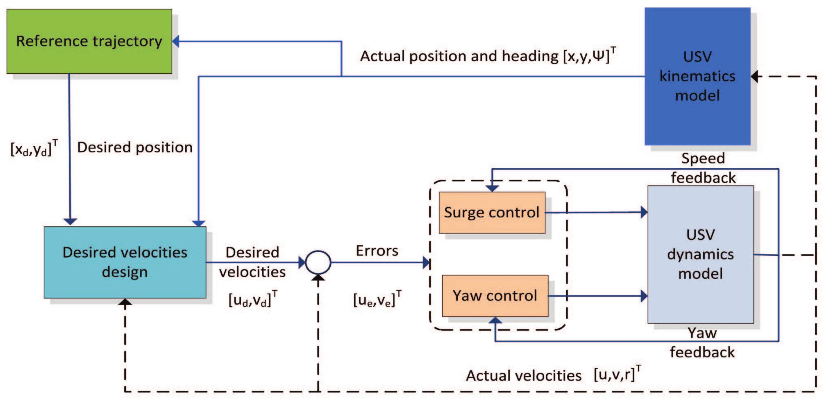
3. Trajectory Tracking Control Design

The sliding mode control (SMC) algorithm is first proposed by Emelyanov in the early 1950s [33], and its advantages are that the algorithm is simple, less computational and has a strong robustness. With the efforts of scientific research all over the world, SMC is gradually applied to the control of robots [34], aircrafts [35], ships [36] and so on. In this section, surge control law and yaw control law are proposed based on a first-order sliding mode and a second-order sliding mode, respectively.

First, define the trajectory tracking error variables:

$$\begin{array}{c}\left\{\begin{array}{c}{x}_e=x-x_d\hfill \\ y_e=y-y_d\hfill \end{array}\right.\end{array}$$

(4)

Taking the time derivative of (4) along (1) produces

$$\begin{array}{c}\left[\begin{array}{c}{\dot{x}}_e\hfill \\ {\dot{y}}_e\hfill \end{array}\right]=\left[\begin{array}{cc}\cos \psi & -\sin \psi \\ \sin \psi & \cos \psi \end{array}\right]\left[\begin{array}{c}u\hfill \\ v\hfill \end{array}\right]-\left[\begin{array}{c}{\dot{x}}_d\hfill \\ {\dot{y}}_d\hfill \end{array}\right]\end{array}$$

(5)

Then, define the velocity tracking error variables:

$$\begin{array}{c}\left\{\begin{array}{c}{u}_e=u-u_d\hfill \\ v_e=v-v_d\hfill \end{array}\right.\end{array}$$

(6)

where $(u_d,v_d)$ are the desired surge velocity and sway velocity.

Assumption 2.

The tracked trajectory is required to be smooth enough. ${\dot{u}}_d$, ${\dot{v}}_d$, ${\dot{x}}_d$, ${\ddot{x}}_d$, ${\dot{y}}_d$ and ${\ddot{y}}_d$ are all bounded.

Consider the following reference trajectory

$$\begin{array}{c}\left\{\begin{array}{c}{x}_d=m(t)+D_1\hfill \\ y_d=n(t)+D_2\hfill \end{array}\right.\end{array}$$

(7)

where $m(t)$ and $n(t)$ are continuous time-varying functions, and $D_1$ and $D_2$ are two constants.

Meanwhile, according to [37], the desired surge velocity and sway velocity are related to $(x_d,y_d)$, and they can be represented as

$$\begin{array}{c}\left\{\begin{array}{c}{u}_d=\cos \psi {\dot{x}}_d+\sin \psi {\dot{y}}_d\hfill \\ v_d=-\sin \psi {\dot{x}}_d+\cos \psi {\dot{y}}_d\hfill \end{array}\right.\end{array}$$

(8)

In this paper, the method to track the reference trajectory is to design the control law to make the $(u_e,v_e)$ converge, and then the convergence of $(x_e,y_e)$ is achieved. Therefore, we assume that $(u_d,v_d)$ is related to $(x_d,y_d)$ and $(x_e,y_e)$, which can be represented as

$$\begin{array}{c}\left\{\begin{array}{c}{u}_d=\cos \psi {\dot{x}}_d+\sin \psi {\dot{y}}_d-k\cos \psi x_e-k\sin \psi y_e\hfill \\ v_d=-\sin \psi {\dot{x}}_d+\cos \psi {\dot{y}}_d+k\sin \psi x_e-k\cos \psi y_e\hfill \end{array}\right.\end{array}$$

(9)

where k is a positive parameter. By simplifying (1), we can get that

$$\begin{array}{c}\left\{\begin{array}{c}u=\cos \psi \dot{x}+\sin \psi \dot{y}\hfill \\ v=-\sin \psi \dot{x}+\cos \psi \dot{y}\hfill \end{array}\right.\end{array}$$

(10)

Based on (9) and (10), (6) can be re-expressed as

$$\begin{array}{c}\left[\begin{array}{c}{u}_e\hfill \\ v_e\hfill \end{array}\right]=\left[\begin{array}{cc}\cos \psi & \sin \psi \\ -\sin \psi & \cos \psi \end{array}\right]\left[\begin{array}{c}{\dot{x}}_e+k{x}_e\hfill \\ {\dot{y}}_e+k{y}_e\hfill \end{array}\right]\end{array}$$

(11)

At the same time, the derivative of $u_d$ and $v_d$ can be represented as

$$\begin{array}{c}\left\{\begin{array}{c}{\dot{u}}_d=\cos \psi {\ddot{x}}_d+\sin \psi {\ddot{y}}_d+v_{d}r-k\cos \psi {\dot{x}}_e-k\sin \psi {\dot{y}}_e\hfill \\ {\dot{v}}_d=-\sin \psi {\ddot{x}}_d+\cos \psi {\ddot{y}}_d-u_{d}r+k\sin \psi {\dot{x}}_e-k\cos \psi {\dot{y}}_e\hfill \end{array}\right.\end{array}$$

(12)

Taking the time derivative of (11) along (2) and (12) produces

$$\begin{array}{c}\left[\begin{array}{c}{\dot{u}}_e\hfill \\ {\dot{v}}_e\hfill \end{array}\right]=\left[\begin{array}{c}r{v}_e\hfill \\ -r{u}_e\hfill \end{array}\right]+\left[\begin{array}{cc}\cos \psi & \sin \psi \\ -\sin \psi & \cos \psi \end{array}\right]\left[\begin{array}{c}{\ddot{x}}_e+k{\dot{x}}_e\hfill \\ {\ddot{y}}_e+k{\dot{y}}_e\hfill \end{array}\right]\end{array}$$

(13)

In the following subsection, surge control law ${\tau }_u$ and yaw control law ${\tau }_r$ will be designed to stabilise the velocity tracking errors $u_e$ and $v_e$, respectively. To facilitate the understanding of the reader, the design block diagram of the trajectory tracking control strategy is shown in Figure 2.

3.1. Surge Control Law

In this subsection, a first-order sliding mode will be employed to design surge control law ${\tau }_u$ to make make $u_e$ converge. At the same time, neural network minimum learning parameter method is used to compensate unknown dynamics and time-varing disturbances online in real time.

Define the first sliding surface

$$\begin{array}{c}{s}_u=u_e+{\lambda }_1{\int }_0^t{u}_e(\mu )d\mu \end{array}$$

(14)

where ${\lambda }_1$ is a positive design parameter. Taking the time derivative of $s_u$ along (13) produces

$$\begin{array}{c}{\dot{s}}_u={\lambda }_1{u}_e+\frac{m_{22}}{m_{11}}vr-\frac{d_{11}}{m_{11}}u-\frac{1}{m_{11}}{\Delta }_u+\frac{1}{m_{11}}{\tau }_u+\frac{1}{m_{11}}{b}_u-{\dot{u}}_d\end{array}$$

(15)

Meanwhile, in order to ensure that the sliding surface can converge to zero within a finite time [38], we define that

$$\begin{array}{c}{\dot{s}}_u=-k_{ue}{s}_u-{\eta }_u\mathrm{sgn}(s_u)\end{array}$$

(16)

where $k_{ue}$ and ${\eta }_u$ are two positive design parameters; $\mathrm{sgn}(•)$ represents the symbol function [36].

Therefore, the corresponding surge control law is selected as

$$\begin{array}{c}{\tau }_u={\tau }_{ue}+{\tau }_{uw}\end{array}$$

(17)

where ${\tau }_{ue}=m_{11}(-\frac{1}{2}{s}_u{\widehat{\varphi }}_u{h}^{T}h-{\lambda }_1{u}_e-\frac{m_{22}}{m_{11}}vr+\frac{d_{11}}{m_{11}}u+{\dot{u}}_d)$ and ${\tau }_{uw}=m_{11}(-k_{ue}{s}_u-{\eta }_u\mathrm{sgn}(s_u))$.

Finally, the update law for the neural network minimum learning parameter method is taken to be

$$\begin{array}{c}{\dot{\widehat{\varphi }}}_u=\frac{{\gamma }_u}{2}{s}_u^2{h}^{T}h-{\kappa }_u{\gamma }_u{\widehat{\varphi }}_u\end{array}$$

(18)

where ${\gamma }_u$ and ${\kappa }_u$ are positive design parameters.

3.2. Yaw Rate Controller

In this subsection, a second-order sliding mode will be employed to design yaw control law ${\tau }_r$ to make $v_e$ converge.

Define the second sliding surface

$$\begin{array}{c}{s}_v={\dot{v}}_e(t)+{\lambda }_2{v}_e(t)+{\lambda }_3{\int }_0^t{v}_e(\mu )d\mu \end{array}$$

(19)

where ${\lambda }_2$ and ${\lambda }_3$ are two positive design parameters. Taking the time derivative of $s_v$ along (13) produces

$$\begin{array}{c}{\dot{s}}_v=\ddot{v}-{\ddot{v}}_d+{\lambda }_2(\dot{v}-{\dot{v}}_d)+{\lambda }_3{v}_e\end{array}$$

(20)

where

$$\begin{array}{cc}\hfill \ddot{v}& ={(-\frac{m_{11}}{m_{22}}ur-\frac{d_{22}}{m_{22}}v-\frac{1}{m_{22}}{\Delta }_v+\frac{b_v}{m_{22}})}^{\prime }\hfill \\ & =(-\frac{m_{11}}{m_{22}}\dot{u}r-\frac{m_{11}}{m_{22}}u(\frac{m_{11}-m_{22}}{m_{33}}uv-\frac{d_{33}}{m_{33}}r+\frac{1}{m_{33}}{\tau }_r-\frac{1}{m_{33}}{\Delta }_r+\frac{1}{m_{33}}{b}_r)-\frac{d_{22}}{m_{22}}\dot{v}-\frac{1}{m_{22}}{\dot{\Delta }}_v+\frac{{\dot{b}}_v}{m_{22}})\hfill \\ & =\frac{1}{m_{22}{m}_{33}}(-m_{11}{m}_{33}\dot{u}r-m_{11}(m_{11}-m_{22})u^{2}v+m_{11}{d}_{22}ur-m_{11}u{\tau }_r+m_{11}u({\Delta }_r-b_r)\hfill \\ & -m_{33}{d}_{22}\dot{v}-m_{33}({\dot{\Delta }}_v-{\dot{b}}_v))\hfill \end{array}$$

(21)

$$\begin{array}{c}{\ddot{v}}_d=v_m-v_n\end{array}$$

(22)

$$\begin{array}{cc}\hfill v_m& =-r[\cos (\psi ){\ddot{x}}_d+\sin (\psi ){\ddot{y}}_d]-\sin (\psi ){}_d+\cos (\psi ){}_d-r[\cos (\psi ){\ddot{x}}_d+\sin (\psi ){\ddot{y}}_d+v_{d}r\hfill \\ & -k(\cos (\psi ){\dot{x}}_e+\sin (\psi ){\dot{y}}_e)]+k[r\cos (\psi ){\dot{x}}_e+\sin (\psi ){\ddot{x}}_e+r\sin (\psi ){\dot{y}}_e-\cos (\psi ){\ddot{y}}_e]\hfill \end{array}$$

(23)

$$\begin{array}{c}{v}_n=u_d\frac{{\tau }_r-d_{33}r+(m_{11}-m_{22})uv}{m_{33}}\end{array}$$

(24)

Based on the above analysis, (20) can be rerepresented as

$$\begin{array}{c}\hfill {\dot{s}}_v=v_b{\tau }_r+v_v-v_m+{\lambda }_2(\dot{v}-{\dot{v}}_d)+{\lambda }_3{v}_e+v_f\end{array}$$

(25)

where $v_b=\frac{(m_{22}{u}_d-m_{11}u)}{m_{22}{m}_{33}}$, $v_v=\frac{-m_{11}{m}_{33}\dot{u}r-m_{11}(m_{11}-m_{22})u^{2}v+m_{11}{d}_{22}ur-m_{33}{d}_{22}\dot{v}-m_{22}{d}_{33}r{u}_d+m_{22}(m_{11}-m_{22})u_{d}uv}{m_{22}{m}_{33}}$ and $v_f=\frac{m_{11}u({\Delta }_r-b_r)-m_{33}({\dot{\Delta }}_v-{\dot{b}}_v)}{m_{22}{m}_{33}}$.

Similarly, in order to ensure that the second-order sliding mode surface can converge in a limited time, one can define that

$$\begin{array}{c}{\dot{s}}_v=-k_{ve}{s}_v-{\eta }_v\mathrm{sgn}(s_v)\end{array}$$

(26)

where $k_{ve}$ and ${\eta }_v$ are two positive design parameters.

Therefore, the corresponding yaw control law is selected as

$$\begin{array}{c}{\tau }_r={\tau }_{re}+{\tau }_{rw}\end{array}$$

(27)

where ${\tau }_{re}=\frac{1}{v_b}(-\frac{1}{2}{s}_v{\widehat{\varphi }}_v{h}^{T}h-v_v+v_m-{\lambda }_2(\dot{v}-{\dot{v}}_d)-{\lambda }_3{v}_e)$ and ${\tau }_{rw}=\frac{1}{v_b}(-k_{ve}{s}_v-{\eta }_v\mathrm{sgn}(s_v))$.

The update law for the neural network minimum learning parameter method is taken to be

$$\begin{array}{c}{\dot{\widehat{\varphi }}}_v=\frac{{\gamma }_v}{2}{s}_v^2{h}^{T}h-{\kappa }_v{\gamma }_v{\widehat{\varphi }}_v\end{array}$$

(28)

where ${\gamma }_v$ and ${\kappa }_v$ are positive design parameters.

Remark 1.

The reason that sliding mode control theory has strong robust ability is that the symbol function can resist unknown dynamics and time-varing disturbances better. However, with the increase of unknown dynamics and time-varing disturbances, this undoubtedly increases the degree of chattering of the control signals. If more than a critical value is exceeded, it will lead to the instability and even collapse of the control system. Therefore, neural network minimum learning parameter method is hired to compensate for unknown dynamics and time-varing disturbances, which undoubtedly reduces the chattering of control signals under the premise of ensuring system robustness.

Remark 2.

Neural network minimum learning parameter method is used instead of the RBF neural network to reduce the computing burden of the controller [22]. At the same time, in the previous literatures [39,40,41], unknown dynamics and external disturbances are compensated separately. However, in this paper, unknown dynamics and time-varing disturbances are packaged together for compensation, which, to a certain extent, can reduce the computation of controller and make it more convenient for engineering implementation. Of course, through qualitative analysis, this paper concludes that the calculation of the burden is reduced, but how much has it been reduced? In future research, the author will give a quantitative analysis.

4. Stability Analysis

The following Theorem 1 presents the stability result of the proposed control law.

Theorem 1.

Consider the closed-loop system consisting of the underactuated USV (1) and (2) satisfying Assumptions 1 and 2, the control laws (17) and (27), the adaptive laws (18) and (28). One can adjust control parameters ${\lambda }_1$, ${\lambda }_2$, ${\lambda }_3$, $k_{ue}$, ${\eta }_u$, ${\gamma }_u$, ${\kappa }_u$, $k_{ve}$, ${\eta }_v$, ${\gamma }_v$ and ${\kappa }_v$, then, all signals in the closed-loop trajectory tracking system for USV are UUB.

Proof of Theorem 1.

Consider the following Lyapunov function candidate:

$$\begin{array}{c}V=\frac{1}{2}(s_u^2+\frac{1}{{\gamma }_u}{\tilde{\varphi }}_u^2+s_v^2+\frac{1}{{\gamma }_v}{\tilde{\varphi }}_v^2)\end{array}$$

(29)

Take the time derivative $\dot{V}$ along (14), (25), we have

$$\begin{array}{cc}\hfill \dot{V}& =s_u{\dot{s}}_u+\frac{1}{{\gamma }_u}{\tilde{\varphi }}_u{\dot{\widehat{\varphi }}}_u+s_v{\dot{s}}_v+\frac{1}{{\gamma }_v}{\tilde{\varphi }}_v{\dot{\widehat{\varphi }}}_v\hfill \\ & =s_u({\lambda }_1{u}_e+\frac{m_{22}}{m_{11}}vr-\frac{d_{11}}{m_{11}}u-\frac{1}{m_{11}}{\Delta }_u+\frac{1}{m_{11}}{\tau }_u+\frac{1}{m_{11}}{b}_u-{\dot{u}}_d)+\frac{1}{{\gamma }_u}{\tilde{\varphi }}_u{\dot{\widehat{\varphi }}}_u\hfill \\ & +s_v(v_b{\tau }_r+v_v-v_m+{\lambda }_2(\dot{v}-{\dot{v}}_d)+{\lambda }_3{v}_e+v_f)+\frac{1}{{\gamma }_v}{\tilde{\varphi }}_v{\dot{\widehat{\varphi }}}_v\hfill \\ & \le \frac{1}{2}{s}_u^2{\varphi }_u{h}^{T}h+\frac{1}{2}+s_u({\lambda }_1{u}_e+\frac{m_{22}}{m_{11}}vr-\frac{d_{11}}{m_{11}}u+{\epsilon }_u+\frac{1}{m_{11}}{\tau }_u-{\dot{u}}_d)+\frac{1}{{\gamma }_u}{\tilde{\varphi }}_u{\dot{\widehat{\varphi }}}_u\hfill \\ & +\frac{1}{2}{s}_v^2{\varphi }_v{h}^{T}h+\frac{1}{2}+s_v(v_b{\tau }_r+v_v-v_m+{\lambda }_2(\dot{v}-{\dot{v}}_d)+{\lambda }_3{v}_e)+\frac{1}{{\gamma }_v}{\tilde{\varphi }}_v{\dot{\widehat{\varphi }}}_v\hfill \\ & \le s_u(\frac{1}{2}{s}_u{\widehat{\varphi }}_u{h}^{T}h+{\lambda }_1{u}_e+\frac{m_{22}}{m_{11}}vr-\frac{d_{11}}{m_{11}}u+{\epsilon }_u+\frac{1}{m_{11}}{\tau }_u-{\dot{u}}_d)-{\tilde{\varphi }}_u(\frac{1}{2}{s}_u^2{h}^{T}h-\frac{1}{{\gamma }_u}{\dot{\widehat{\varphi }}}_u)\hfill \\ & +s_v(\frac{1}{2}{s}_v{\widehat{\varphi }}_v{h}^{T}h+v_b{\tau }_r+v_v-v_m+{\lambda }_2(\dot{v}-{\dot{v}}_d)+{\lambda }_3{v}_e)-{\tilde{\varphi }}_v(\frac{1}{2}{s}_v^2{h}^{T}h-\frac{1}{{\gamma }_v}{\dot{\widehat{\varphi }}}_v)+1\hfill \end{array}$$

(30)

Submitting the control laws (17), (27) and adaptive laws (18), (28) yields

$$\begin{array}{c}\hfill \dot{V}\le -k_{ue}{s}_u^2-{\kappa }_u{\tilde{\varphi }}_u{\widehat{\varphi }}_u-({\eta }_u-{\epsilon }_u)\left|s_u\right|-k_{ve}{s}_v^2-{\kappa }_v{\tilde{\varphi }}_v{\widehat{\varphi }}_v-({\eta }_v-{\epsilon }_v)\left|s_v\right|+1\end{array}$$

(31)

Because ${({\tilde{\varphi }}_{\iota }+{\varphi }_{\iota })}^2\ge 0$, then ${\tilde{\varphi }}_{\iota }^2+{\varphi }_{\iota }^2+2{\tilde{\varphi }}_{\iota }({\widehat{\varphi }}_{\iota }-{\tilde{\varphi }}_{\iota })\ge 0$. One can get that $2{\tilde{\varphi }}_{\iota }{\widehat{\varphi }}_{\iota }\ge {\tilde{\varphi }}_{\iota }^2-{\varphi }_{\iota }^2$, where $\iota =u$ and v.

Moreover, define ${\eta }_u>{\epsilon }_u$ and ${\eta }_v>{\epsilon }_v$, then (32) can be obtained.

$$\begin{array}{c}\dot{V}\le -k_{ue}{s}_u^2-k_{ve}{s}_v^2-\frac{1}{2}{\kappa }_u{\tilde{\varphi }}_u^2-\frac{1}{2}{\kappa }_v{\tilde{\varphi }}_v^2+\frac{1}{2}{\kappa }_u{\varphi }_u^2+\frac{1}{2}{\kappa }_v{\varphi }_v^2+1\end{array}$$

(32)

Define $l_1=k_{ue}$, $l_2=k_{ve}$, $l_3=\frac{1}{2}{\kappa }_u$, $l_4=\frac{1}{2}{\kappa }_v$, $\nabla =\frac{1}{2}{\kappa }_u{\varphi }_u^2+\frac{1}{2}{\kappa }_v{\varphi }_v^2+1$, then (32) becomes

$$\begin{array}{c}\dot{V}\le -l_1{s}_u^2-l_2{s}_v^2-l_3{\tilde{\varphi }}_u^2-l_4{\tilde{\varphi }}_v^2+\nabla \end{array}$$

(33)

Define $l=\min \{l_1,l_2,l_3,l_4\}$, then it follows from (33) that

$$\begin{array}{c}\dot{V}\le -2lV+\nabla \end{array}$$

(34)

Solving inequality (34) gives

$$\begin{array}{c}V\le (V(0)-\frac{\nabla }{2l})e^{-2lt}+\frac{\nabla }{2l}\le V(0)e^{-2lt}+\frac{\nabla }{2l},\forall t>0\end{array}$$

(35)

Through the analysis of inequality (35) we can draw that V is eventually bounded by $\frac{\nabla }{2l}$. Thus, all the error signals in the closed loop system are UUB. In the strict sense, in the case of continuous optimization of the control parameters, $\frac{\nabla }{2l}$ can be made arbitrarily small, thus, more accurate trajectory tracking performance is obtained. ☐

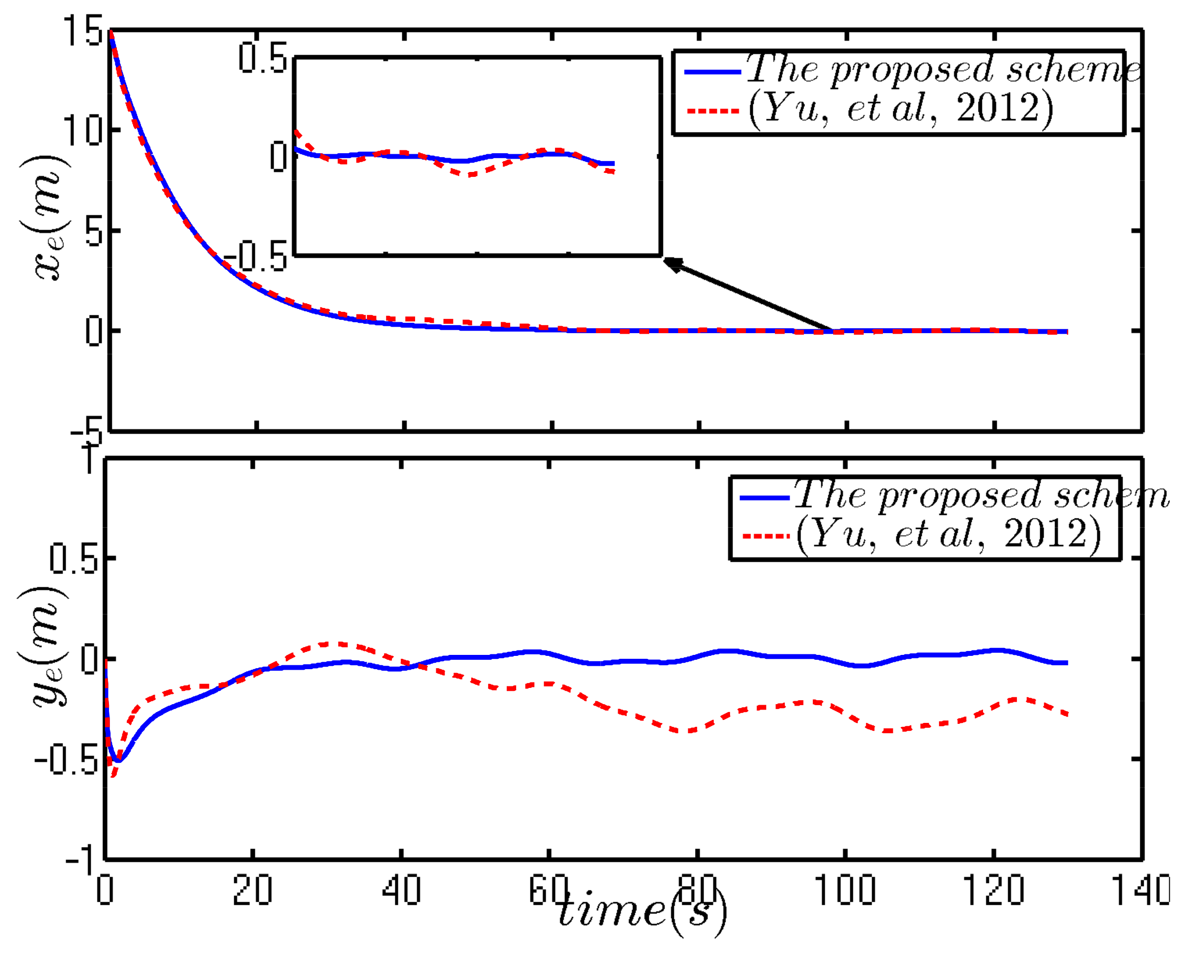
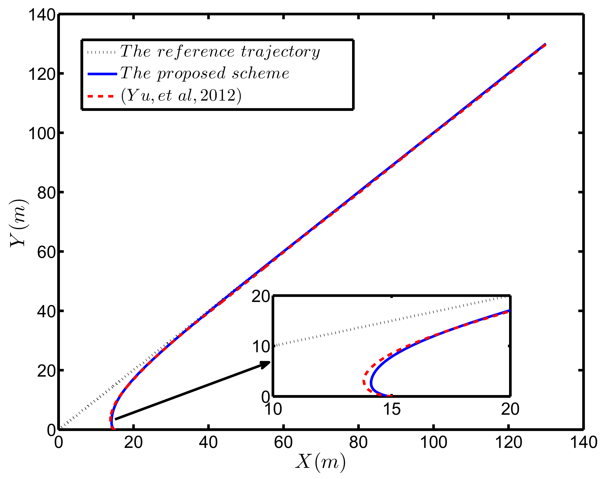
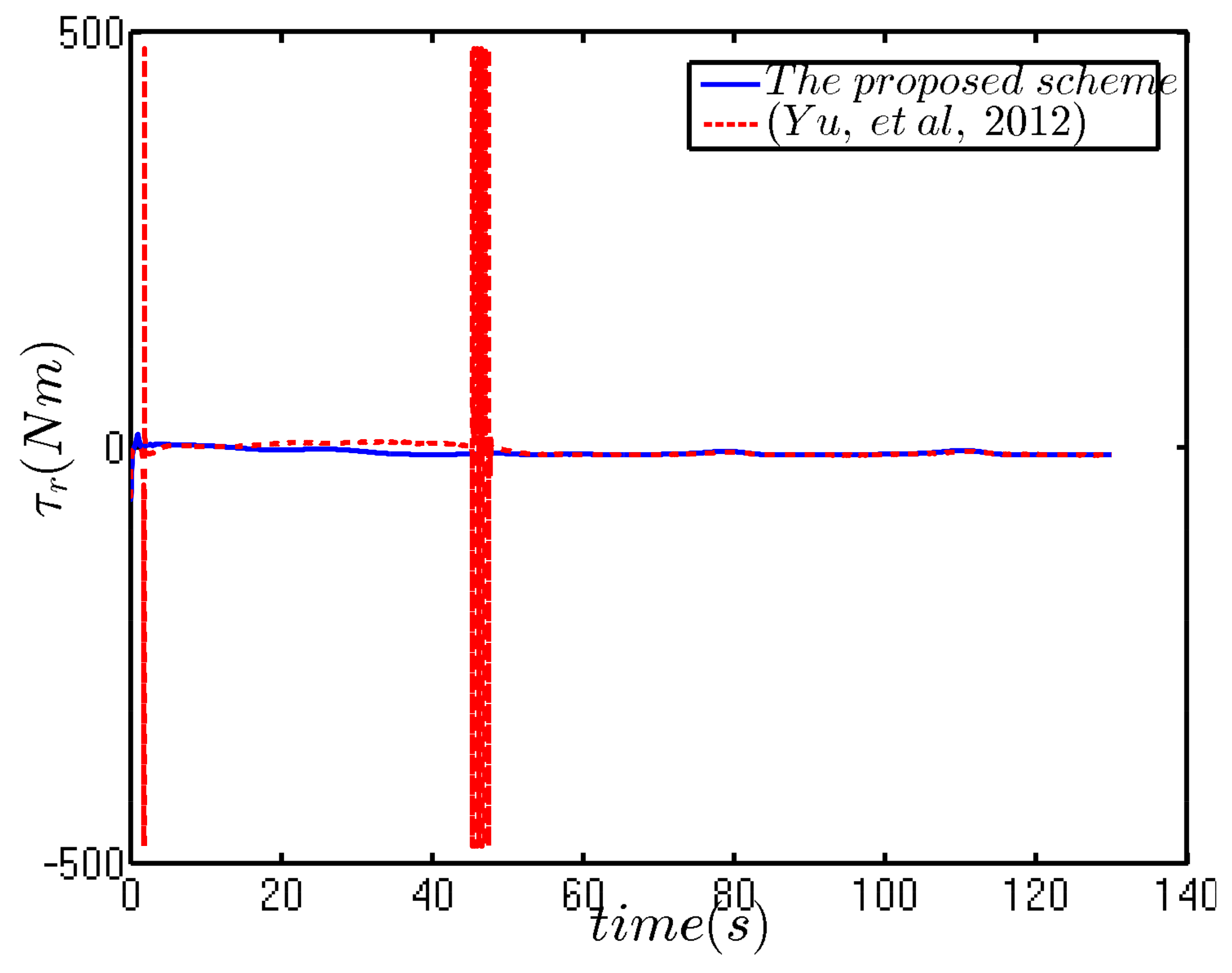
5. Numerical Simulations

In this section, the numerical simulations of straight line trajectory and circle trajectory tracking are given to prove the correctness and effectiveness of the adaptive trajectory tracking control law. Meanwhile, in order to prove the superiority of the control strategy proposed in this paper, compare it with the [21] (Yu, et al., 2012) that deals with unknown dynamics and disturbances only with the robustness of sliding mode. For this purpose, the underactuated USV (length of 1.255 m, breadth of 0.29 m, mass of 23.8 kg) is selected as the same as that in [42,43,44].

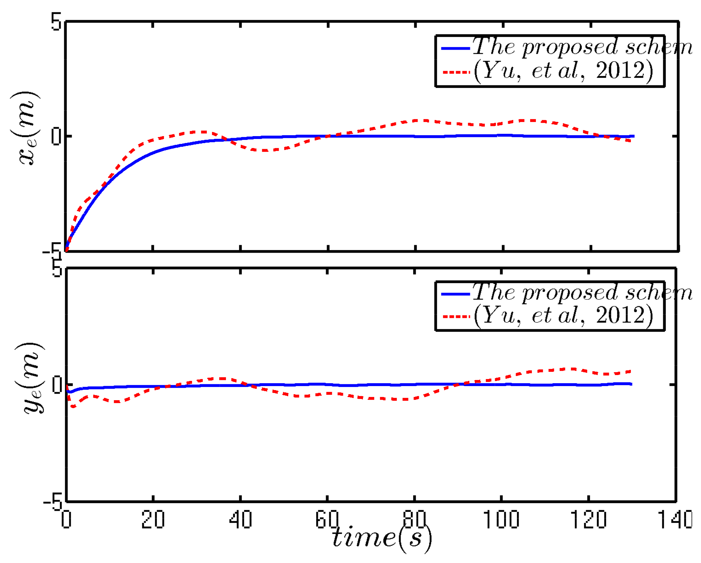
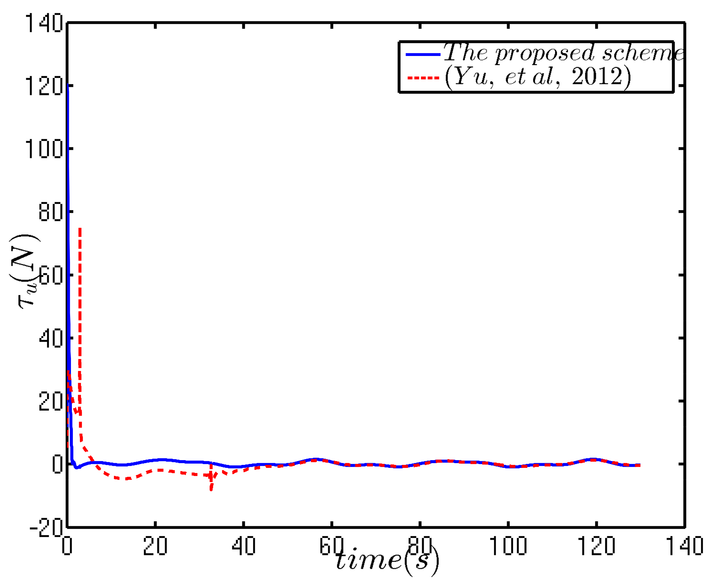
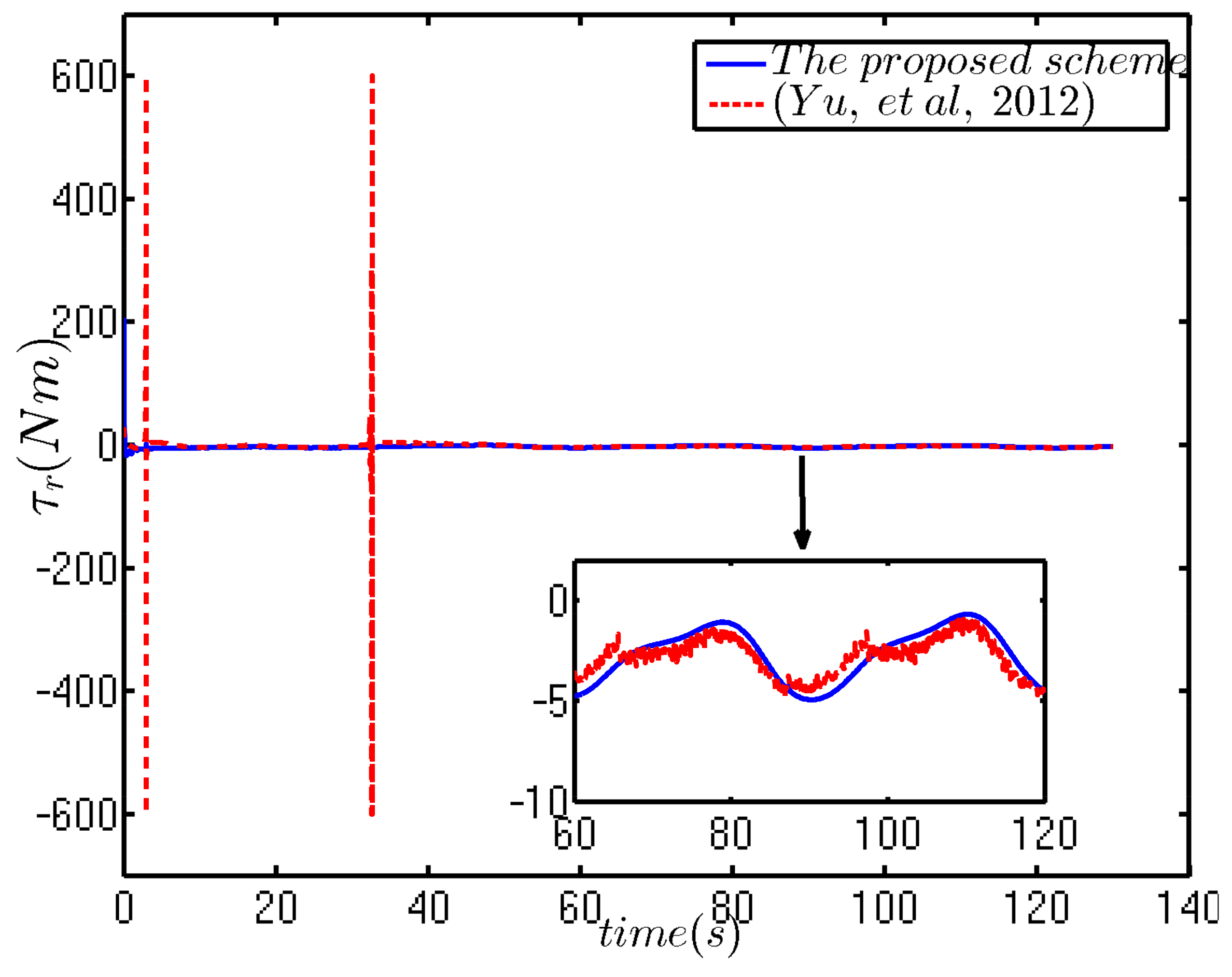
5.1. Tracking a Straight Line

In the previous approach [45], the straight line trajectory cannot be tracked because of the requirement of zero-yaw velocity. First, a simple straight line is regarded as a reference trajectory, which is described as $x_d=t$, $y_d=t$. According to [42,43,44], the external disturbances are assumed to be $b_u=1+0.5\sin (0.2t)+0.3\cos (0.5t)$, $b_v=1+0.5\sin (0.2t)+0.3\cos (0.4t)$, $b_r=1+0.2\sin (0.1t)+0.2\cos (0.2t)$, that is a time-varying disturbances. Meanwhile, ${\Delta }_u=0.2f_u$, ${\Delta }_v=0.2f_v$ and ${\Delta }_r=0.2f_r$. The initial state of USV is $[x(0),y(0),\psi (0),u(0),v(0),r(0)]=[15\mathrm{m},0\mathrm{m},0\mathrm{rad},0\mathrm{m}/\mathrm{s},0\mathrm{m}/\mathrm{s},0\mathrm{rad}/\mathrm{s}]$. The control parameters used in the controller are $k=0.1$, ${\lambda }_1=1$, ${\lambda }_2=5$, ${\lambda }_3=1$, $k_{\mathrm{u}e}=0.01$, $k_{ve}=0.015$, ${\eta }_u=0.001$, ${\eta }_v=0.001$, ${\gamma }_u=1$, ${\gamma }_v=1$, ${\kappa }_u=0.01$ and ${\kappa }_v=0.01$. The comparison results of the numerical simulation are provided in Figure 3, Figure 4, Figure 5 and Figure 6.

Figure 3 depicts the trajectory tracking in two-dimensional plane, where the reference trajectory is a straight line. Despite the presence of unknown dynamics and non measurable external disturbances, the proposed control scheme still has a good performance. Besides, the control strategy of (Yu, et al., 2012) also has a good result. Figure 4 shows the comparison results of tracking errors. It can be observed that the tracking errors of the proposed scheme and (Yu, et al., 2012) both can converge well near the zero point, but it is obvious that the errors range of the proposed scheme have a smaller fluctuation range. Figure 5 and Figure 6 demonstrate the force ${\tau }_u$ and the moment ${\tau }_r$ respectively. Furthermore, one can get that compared with the method proposed in this paper, the control inputs of (Yu, et al., 2012) have a larger chattering phenomenon. For the control system, the chattering is not conducive to the stability of the system. For the actuator, frequent chattering will aggravate the wear of the actuator, which is not conducive to the implementation of the engineering.

5.2. Tracking a Circle

In the case of USV initial conditions, the control parameters and external disturbances do not make any changes, a circle trajectory tracking simulation experiment with a radius of 20 m is carried out to further verify the correctness of the proposed scheme. The reference trajectory is described as $x_d=20\cos (0.05t)$, $y_d=20\sin (0.05t)$. The tracking results are shown in Figure 7, Figure 8, Figure 9 and Figure 10.

Although no adjustments have been made to the control parameters, it can be seen from Figure 7 that the proposed scheme and (Yu, et al., 2012) still have satisfactory tracking results, which show that they have good generality. Figure 8 plots the tracking errors of the proposed scheme and (Yu, et al., 2012). It can be observed that the proposed scheme can keep $x_e$ and $y_e$ stable near the equilibrium point and they have very small fluctuations. However, the performance of (Yu, et al., 2012) is not so satisfactory. Figure 9 and Figure 10 depict the comparison results of control inputs. Notice from the simulation results that similar to the straight line tracking, the (Yu, et al., 2012) control inputs ${\tau }_u$ and ${\tau }_r$ generate large chattering phenomena, which are not allowed in actual engineering.

Thus far, the numerical simulations of straight line trajectory tracking and circle trajectory tracking have achieved good results, indicating the superiority and robustness of adaptive trajectory tracking control strategy proposed in this paper.

6. Conclusions

This paper has proposed an adaptive trajectory tracking control strategy for an underactuated USV subject to unknown dynamics and time-varing external disturbances. The scheme is presented by combing first-order sliding mode, second-order sliding mode and neural network minimum learning parameter method, which is obviously different from traditional trajectory tracking control approach. Neural network minimum learning parameter method is introduced into the design of controller. It not only handles the problems of unknown dynamics and external disturbances, but also enhances the robustness of control strategy, and also reduces chattering phenomenon of control signals to some extent. Comparison results of numerical simulation verify the effectiveness and correctness of the proposed method. Although this article has taken more of the actual situation into consideration, there are still a lot of problems that need to be resolved. For example, the reduced amount of the controller’s calculation burden is not given quantificationally. This is also one of the future research directions.

References

1. Sinisterra, A.J.; Dhanak, M.R.; Ellenrieder, K.V. Stereovision-based target tracking system for USV operations. Ocean Eng. 2017, 133, 197–214. [Google Scholar] [CrossRef]
2. Fan, Y.; Mu, D.; Zhang, X.; Wang, G.; Guo, C. Course keeping Control Based on Integrated Nonlinear Feedback for a USV with Pod-like Propulsion. J. Navig. 2018, 1–21. [Google Scholar] [CrossRef]
3. Specht, C.; Świtalski, E.; Specht, M. Application of an Autonomous/Unmanned Survey Vessel (ASV/USV) in Bathymetric Measurements. Pol. Marit. Res. 2017, 24, 36–44. [Google Scholar] [CrossRef]
4. Sun, X.; Wang, G.; Fan, Y.; Mu, D.; Qiu, B. An Automatic Navigation System for Unmanned Surface Vehicles in Realistic Sea Environments. Appl. Sci. 2018, 8, 193. [Google Scholar]
5. Vivone, G.; Braca, P.; Horstmann, J. Knowledge-Based Multitarget Ship Tracking for HF Surface Wave Radar Systems. Trans. Geosci. Remote Sens. 2015, 53, 3931–3949. [Google Scholar] [CrossRef]
6. Liu, C.; Zou, Z.; Hou, X. Stabilization And Tracking Of Underactuated Surface Vessels In Random Waves With Fin Based On Adaptive Hierarchical Sliding Mode Technique. Asian J. Control 2015, 16, 1492–1500. [Google Scholar] [CrossRef]
7. Gao, T.; Huang, J.; Zhou, Y.; Song, Y.D. Robust adaptive tracking control of an underactuated ship with guaranteed transient performance. Int. J. Syst. Sci. 2016, 48, 272–279. [Google Scholar] [CrossRef]
8. Do, K.D. Global robust adaptive path-tracking control of underactuated ships under stochastic disturbances. Ocean Eng. 2016, 111, 267–278. [Google Scholar] [CrossRef]
9. Zhang, G.; Zhang, X. Concise Robust Adaptive Path-Following Control of Underactuated Ships Using DSC and MLP. IEEE J. Ocean. Eng. 2014, 39, 685–694. [Google Scholar] [CrossRef]
10. Jiang, Z.P. Controlling Underactuated Mechanical Systems: A Review and Open Problems. In Advances in the Theory of Control, Signals and Systems with Physical Modeling; Springer: Berlin/Heidelberg, Germany, 2010; pp. 77–88. [Google Scholar]
11. Zheng, Z.W.; Huo, W. Trajectory tracking control for underactuated stratospheric airship. Adv. Space Res. 2012, 50, 906–917. [Google Scholar] [CrossRef]
12. Harmouche, M.; Laghrouche, S.; Chitour, Y. Global tracking for underactuated ships with bounded feedback controllers. Int. J. Control 2014, 87, 2035–2043. [Google Scholar] [CrossRef]
13. Do, K.D.; Pan, J. Underactuated ships follow smooth paths with Integral actions and without velocity measurements for feedback: Theory and experiments. IEEE Trans. Control Syst. Technol. 2006, 14, 308–322. [Google Scholar] [CrossRef]
14. Ghommam, J.; Mnif, F.; Derbel, N. Global stabilisation and tracking control of underactuated surface vessels. IET Control Theory Appl. 2010, 4, 71–88. [Google Scholar] [CrossRef]
15. Chwa, D. Global Tracking Control of Underactuated Ships With Input and Velocity Constraints Using Dynamic Surface Control Method. IEEE Trans. Control Syst. Technol. 2011, 19, 1357–1370. [Google Scholar] [CrossRef]
16. Sonnenburg, C.R.; Woolsey, C.A. Modeling, Identification, and Control of an Unmanned Surface Vehicle. J. Field Robot. 2013, 30, 371–398. [Google Scholar] [CrossRef]
17. Wu, Y.; Zhang, Z.; Xiao, N. Global Tracking Controller for Underactuated Ship via Switching Design. J. Dyn. Syst. Meas. Control 2014, 136, 054506. [Google Scholar] [CrossRef]
18. Dong, Z.; Wang, L.; Li, Y.; Liu, T.; Zhang, G. Trajectory tracking control of underactuated USV based on modified backstepping approach. Int. J. Nav. Archit. Ocean Eng. 2015, 7, 817–832. [Google Scholar] [CrossRef]
19. Yang, Y.; Du, J.; Liu, H.; Guo, C.; Abrahham, A. A trajectory tracking robust controller of surface vessels with disturbance uncertainties. IEEE Trans. Control Syst. Technol. 2014, 22, 1511–1518. [Google Scholar] [CrossRef]
20. Liu, C.; Zou, Z.; Yin, J. Trajectory tracking of underactuated surface vessels based on neural network and hierarchical sliding mode. J. Mar. Sci. Technol. 2015, 20, 322–330. [Google Scholar] [CrossRef]
21. Yu, R.; Zhu, Q.; Xia, G.; Liu, Z. Sliding mode tracking control of an underactuated surface vessel. IET Control Theory Appl. 2012, 6, 461–466. [Google Scholar] [CrossRef]
22. Mu, D.; Wang, G.; Fan, Y.; Sun, X.; Qiu, B. Adaptive LOS Path Following for a Podded Propulsion Unmanned Surface Vehicle with Uncertainty of Model and Actuator Saturation. Appl. Sci. 2017, 7, 1232. [Google Scholar] [CrossRef]
23. Hassan, M.; Hamada, M. A Neural Networks Approach for Improving the Accuracy of Multi-Criteria Recommender Systems. Appl. Sci. 2017, 7, 868. [Google Scholar] [CrossRef]
24. Li, Y.; Tong, S. Adaptive Fuzzy Output Constrained Control Design for Multi-Input Multioutput Stochastic Nonstrict-Feedback Nonlinear Systems. IEEE Trans. Cybern. 2017, 47, 4086–4095. [Google Scholar] [CrossRef] [PubMed]
25. Li, Y.; Tong, S. Fuzzy Adaptive Control Design Strategy of Nonlinear Switched Large-Scale Systems. IEEE Trans. Syst. Man Cybern. Syst. 2017, 99, 107–117. [Google Scholar] [CrossRef]
26. Zhang, G.; Zhang, X. Concise adaptive fuzzy control of nonlinearly parameterized and periodically time-varying systems via small gain theory. Int. J. Control Autom. Syst. 2016, 14, 1–13. [Google Scholar] [CrossRef]
27. Pan, C.Z.; Lai, X.Z.; Yang, S.X.; Wu, M. An efficient neural network approach to tracking control of an autonomous surface vehicle with unknown dynamics. Expert Syst. Appl. Int. J. 2013, 40, 1629–1635. [Google Scholar] [CrossRef]
28. Fossen, T.I. Handbook of Marine Craft Hydrodynamics and Motion Control; Wiley: New York, NY, USA, 2011; ISBN 978-1119991496. [Google Scholar]
29. Liu, C.; Ding, W.; Li, Z.; Yang, C. Prediction of high-speed grinding temperature of titanium matrix composites using BP neural network based on PSO algorithm. Int. J. Adv. Manuf. Technol. 2016, 89, 1–9. [Google Scholar] [CrossRef]
30. Jiang, G.; Luo, M.; Bai, K.; Chen, S. A Precise Positioning Method for a Puncture Robot Based on a PSO-Optimized BP Neural Network Algorithm. Appl. Sci. 2017, 7, 969. [Google Scholar] [CrossRef]
31. Mu, D.D.; Wang, G.F.; Fan, Y.S. Design of Adaptive Neural Tracking Controller for Pod Propulsion Unmanned Vessel Subject to Unknown Dynamics. J. Electr. Eng. Technol. 2017, 12, 2365–2377. [Google Scholar]
32. Zhang, G.; Zhang, X. A novel DVS guidance principle and robust adaptive path-following control for underactuated ships using low frequency gain-learning. ISA Trans. 2015, 56, 75–85. [Google Scholar] [CrossRef] [PubMed]
33. Emelyanov, S.V. Automatic control systems with variable structure. Autom. Control Syst. Var. Struct. 1970, 4, 75–85. [Google Scholar]
34. Khosravi, S.; Jahangir, M.; Afkhami, H. Adaptive Fuzzy SMC-Based Formation Design for Swarm of Unknown Time-Delayed Robots. Nonlinear Dyn. 2012, 4, 139–143. [Google Scholar] [CrossRef]
35. Li, S.; Wang, Y.; Tan, J.; Zheng, Y. Adaptive RBFNNs/integral sliding mode control for a quadrotor aircraft. Neurocomputing 2016, 216, 126–134. [Google Scholar] [CrossRef]
36. Mu, D.; Wang, G.; Fan, Y.; Zhao, Y. Modeling and Identification of Podded Propulsion Unmanned Surface Vehicle and Its Course Control Research. Math. Probl. Eng. 2017, 2, 1–13. [Google Scholar] [CrossRef]
37. Ashrafiuon, H.; Muske, K.R.; Mcninch, L.C.; Soltan, R.A. Sliding-Mode Tracking Control of Surface Vessels. IEEE Trans. Ind. Electron. 2008, 55, 4004–4012. [Google Scholar] [CrossRef]
38. Iqbal, J.; Zuhaib, K.; Han, C.; Khan, A.; Ali, M. Adaptive Global Fast Sliding Mode Control for Steer-by-Wire System Road Vehicles. Appl. Sci. 2017, 7, 738. [Google Scholar] [CrossRef]
39. Zhang, G.; Zhang, X.; Zheng, Y. Adaptive neural path-following control for underactuated ships in fields of marine practice. Ocean Eng. 2015, 104, 558–567. [Google Scholar] [CrossRef]
40. Li, J.H.; Lee, P.M.; Jun, B.H.; Lin, Y.K. Point-to-point navigation of underactuated ships. Automatica 2008, 44, 207–214. [Google Scholar] [CrossRef]
41. Liu, L.; Wang, D.; Peng, Z. Path following of marine surface vehicles with dynamical uncertainty and time-varying ocean disturbances. Neurocomputing 2016, 173, 799–808. [Google Scholar] [CrossRef]
42. Pan, C.Z.; Lai, X.Z.; Yang, S.X.; Wu, M. A biologically inspired approach to tracking control of underactuated surface vessels subject to unknown dynamics. Expert Syst. Appl. Int. J. 2015, 42, 2153–2161. [Google Scholar] [CrossRef]
43. Hu, X.; Du, J.; Sun, Y. Robust Adaptive Control for Dynamic Positioning of Ships. IEEE J. Ocean. Eng. 2017, 99, 1–10. [Google Scholar] [CrossRef]
44. Du, J.; Hu, X.; Krstić, M.; Sun, Y. Robust dynamic positioning of ships with disturbances under input saturation. Automatica 2016, 73, 207–214. [Google Scholar] [CrossRef]
45. Lefeber, E.; Pettersen, K.Y.; Nijmeijer, H. Tracking control of an underactuated ship. IEEE Trans. Control Syst. Technol. 2003, 11, 52–61. [Google Scholar] [CrossRef]
Figure 1. The earth-fixed inertial and body-fixed frame.
Applsci 08 00547 g001
Figure 2. Block diagram of trajectory tracking control strategy.
Applsci 08 00547 g002
Figure 3. Comparison results of straight line trajectory tracking.
Applsci 08 00547 g003
Figure 4. Comparison results of tracking errors.
Applsci 08 00547 g004
Figure 5. Comparison results of τ u .
Applsci 08 00547 g005
Figure 6. Comparison results of τ r .
Applsci 08 00547 g006
Figure 7. Comparison results of circle trajectory tracking.
Applsci 08 00547 g007
Figure 8. Comparison results of tracking errors.
Applsci 08 00547 g008
Figure 9. Comparison results of τ u .
Applsci 08 00547 g009
Figure 10. Comparison results of τ r .
Applsci 08 00547 g010