Study of the Ultimate Error of the Axis Tolerance Feature and Its Pose Decoupling Based on an Area Coordinate System

Abstract

Manufacturing error and assembly error should be taken into consideration during evaluation and analysis of accurate product performance in the design phase. Traditional tolerance analysis methods establish error propagation model based on dimension chains with tolerance values being regarded as error boundaries, and obtain the limit of target feature error through optimization methods or conducting statistical analysis with the tolerance domain being the boundary. As deviations of the tolerance feature (TF) on degrees of freedom (DOF) have coupling relations, accurate deviations on all DOF may not be obtained, even though these deviations constitute the basis for product performance analysis. Therefore, taking the widely used shaft-hole fit as an example, a pose decoupling model of the axis TF was proposed based on an area coordinate system. This model realized decoupling analysis of any pose of the axis TF within the tolerance domain. As proposed by the authors, by combining a tolerance analysis model based on tracking local coordinate systems, ultimate pose analysis of the closed-loop system, namely the target feature, as well as statistical analysis could be further implemented. This method contributed to analysis of true product performance with arbitrary error in the product design phase from the angle of tolerance, therefore, shortening the product research and development cycle. This method is demonstrated through applying it to a real-life example.

1. Introduction

Shaft-hole fit is a common form of fitting in rotating mechanical products. Dimension error, geometric shape error, and fit error of shafts and holes are important sources of assembly error [1,2,3]. They directly affect the assembly accuracy, kinematic accuracy and service life of products, for example, the rotation accuracy of a machine tool spindle, gear transmission error, and service life of the bearing [4]. Therefore, it is necessary to discuss the relationship between assembly system performance and geometric and fit error of the shaft-hole.

Historically, scholars have conducted extensive research work on this issue. However, most studies have focused on the tolerance analysis of assembly systems, including the Direct Linearization Method [5], Matrix method [6], Unified Jacobian-Torsor method [7], and the Small Displacement Torsor method [8]. Assembly error with clearance fit is mainly studied by equivalent substitution. For example, Desrochers et al. [9] proposed the Matrix method to view shaft-hole clearance fit into coaxiality tolerance. Chase et al. [5] regarded different fit states in all kinds of kinematic pairs according to the Direct Linearization Method. Desrochers et al. [7] expressed the contact and kinematic relationship between fitting parts by the Torsor method. They established error propagation models based on the dimension chain, which regard the tolerance value and clearance value as constrained boundaries for variation in the tolerance feature (TF) through an optimization method or conducting statistical analysis with the tolerance domain being the boundary, so as to realize error analysis of the assembly system [10].

Tolerance analysis models like the Matrix method and the Small Displacement Torsor method give a range of 12 ultimate values for TF from the angle of six degrees of freedom (DOF). Influenced by the principle of the algorithm itself, the search for the limiting state of TF by the optimization method is probably formed by multiple uncertain combinations of deviations on multiple DOF, but it does not determined the limit deviation from the expected DOF. Therefore, when the limiting situation or statistical situation for all kinds of product performances with errors such as the kinematics and dynamical properties, is carried out in the product design phase, input parameters may not be accurate enough and will affect the accuracy of the analysis results. Therefore, before performance analysis of products with errors, pose (position and orientation [11]) decoupling on six spatial DOF must be implemented for TF so that the actual deviations of TF on all DOF are obtained [12,13]. In this way, the error range of the target feature can be more accurately obtained and this range should be smaller than error ranges given by the Matrix method and the Small Displacement Torsor method, etc. Moreover, explicit analytic expression of target feature error can be obtained, especially when ultimate error is not solved through optimized mathematical iteration method. Thus, explicit solutions for six DOF at arbitrary positions, including the limiting position of TF, can be realized.

Currently, when prediction and analysis of the mechanical properties of assembly systems with errors is conducted in the product design phase, the error value is usually manually set [14], and it is not derived from tolerance values given by designers. Therefore, in order to explore a method which establishes the relation between tolerance of part of the dimension chain and performance of the assembly system, TF of shaft-hole fit-axis TF [15] was taken as an example in this paper, to examine a pose decoupling model. Inspiration for this method came from the Tolerance-Map (T-Map) model proposed by Davidson et al. [16] and the Deviation-Domain model proposed by Giordano et al. [15]. The two methods are still essentially tolerance analysis methods. The T-Map model is a widely used method which uses a hypothetical Euclidean point-space of a convex polyhedron and is completely compatible with ASME Y 14.5-1994 standards.

Its shape, dimension and internal subset reflect TF type, size, shape and all possible variations of pose [17]. The variation range of each TF which is gained by the T-Map model through the area coordinate system is also called the convex hull. Points in the convex hull have a one-to-one mapping relation with all possible error variations of TFs in the tolerance zone. T-Map uses the Minkowski mum algorithm to calculate the ultimate variation of the target feature. This algorithm scans vertexes and boundaries of the convex hull along the dimension chain of TFs one by one in a recursive manner, finally getting the convex hull which describes variations of the target feature. This is a model that calculates the boundaries of target feature variation by geometric operation. The calculation load of Minkowski sum shows exponential growth with the increase in component links in the dimension chain. The calculation load for complicated dimension chains is extremely good. As the T-Map method does not suggest an analytical model between the convex hull vertex of the target feature and the convex hull vertex of each TF on the dimension chain, deviation data expressed by the convex hull vertex of each TF and any point within the convex hull cannot be used in product performance analysis.

Therefore, based on the T-Map, the area coordinate system was used in this paper to study a shaft-hole relative pose description method with the existence of tolerance and clearance fit. The mapping relationship between the area coordinate system and Cartesian coordinate system was further established for each TF on the dimension chain. A tolerance analysis model based on tracking local coordinate systems [18], as proposed previously, was combined to obtain analytic expression of pose decoupling of the axis TF as expressed by the area coordinate system. This method not only accurately obtained the ultimate error of the target feature through permutation and combination of ultimate area coordinate values, with a greatly reduced calculated quantity when compared with the T-Map method, but also obtained the sole deviation value of TF on arbitrary DOF within the tolerance domain by changing the corresponding area coordinate value. Therefore, it provides the foundations for accurate analysis of product performance.

2. Error Transformation Matrix of Axis TF

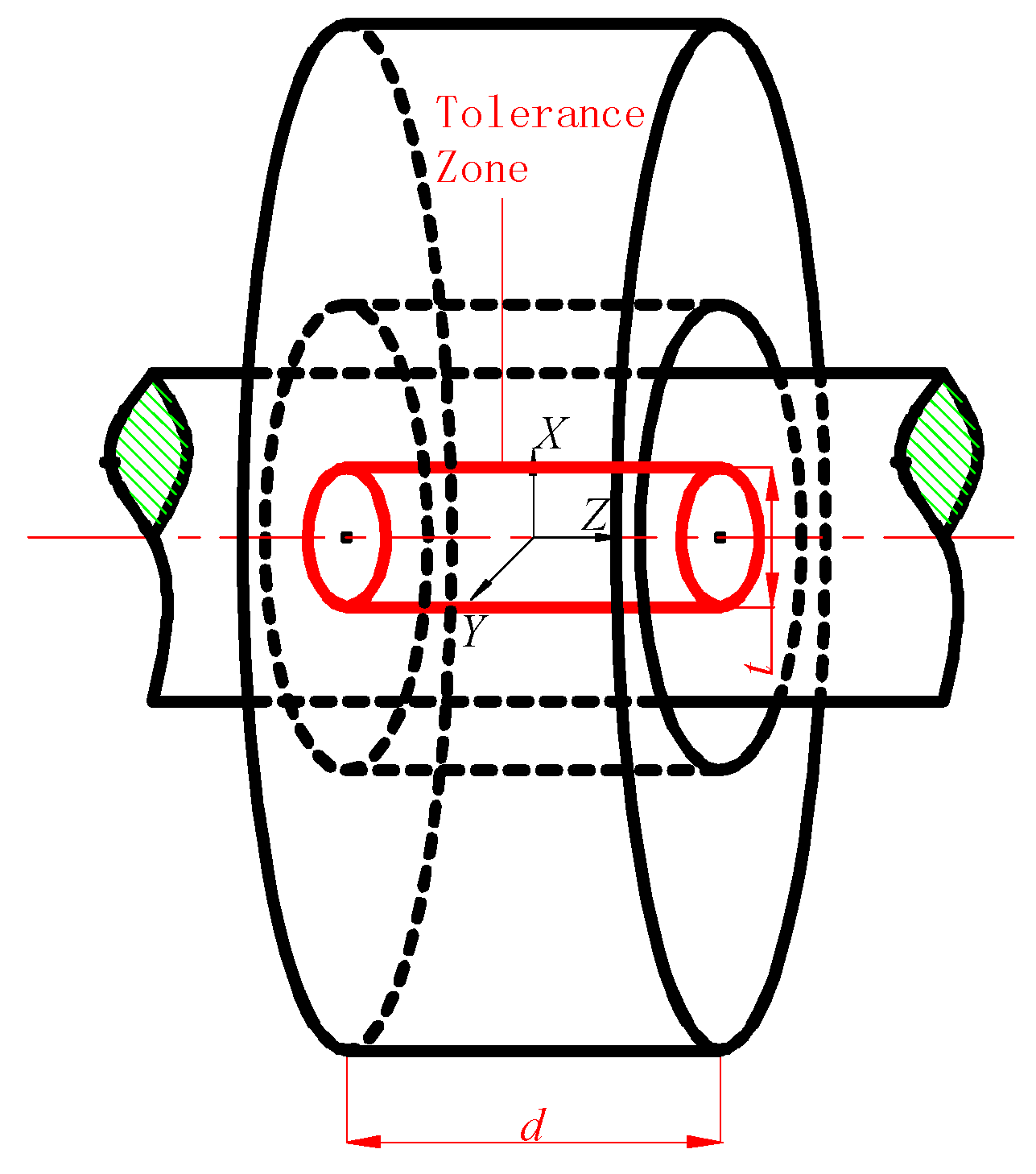
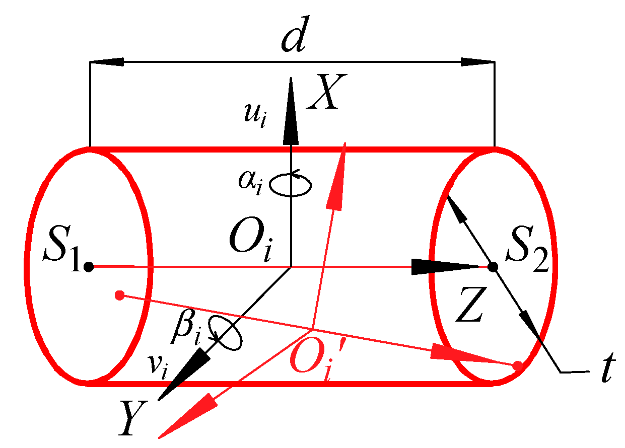
For shaft-hole fit (Figure 1), the cylinder tolerance zone is acquired by expressing clearance value at the axis, so the variation of shaft in the hole is equivalent to the variation of the axis in the cylinder tolerance zone in Figure 2. During tolerance analysis, the error transformation matrix D_i reflects variation of TF [18]. D_i is gained from homogeneous transform matrix (HTM) based on DOF. According to TTRS(Technologically and Topologically Related Surfaces) theory [9], the axis TF in Figure 2 has four DOFs in the Cartesian coordinate system O-XYZ, including the horizontal displacement u_i, v_i along X and Y axes as well as rotation α_i, β_i around X and Y axes. Basic HTMs on these four DOFs are:

$$\begin{gathered} \mathit{T}\mathit{r}\mathit{a}\mathit{n}\mathit{s}\left(u_i\right)=\left[\begin{array}{cccc}1& 0& 0& u_i\\ 0& 1& 0& 0\\ 0& 0& 1& 0\\ 0& 0& 0& 1\end{array}\right] , \mathit{T}\mathit{r}\mathit{a}\mathit{n}\mathit{s}\left(v_i\right)=\left[\begin{array}{cccc}1& 0& 0& 0\\ 0& 1& 0& v_i\\ 0& 0& 1& 0\\ 0& 0& 0& 1\end{array}\right] \\ \mathit{R}\mathit{o}\mathit{t}\left({\alpha }_i\right)=\left[\begin{array}{cccc}1& 0& 0& 0\\ 0& \cos {\alpha }_i& -\sin {\alpha }_i& 0\\ 0& \sin {\alpha }_i& \cos {\alpha }_i& 0\\ 0& 0& 0& 1\end{array}\right] , \mathit{R}\mathit{o}\mathit{t}\left({\beta }_i\right)=\left[\begin{array}{cccc}\cos {\beta }_i& 0& \sin {\beta }_i& 0\\ 0& 1& 0& 0\\ -\sin {\beta }_i& 0& \cos {\beta }_i& 0\\ 0& 0& 0& 1\end{array}\right] \end{gathered}$$

(1)

Due to small errors, $\sin {\alpha }_i\approx {\alpha }_i$ and $\cos {\alpha }_i\approx 1$. These are similar to ${\beta }_i$. Therefore, the corresponding error transformation matrix D_i is:

$${\mathit{D}}_{\mathit{i}}=\mathit{T}\mathit{r}\mathit{a}\mathit{n}\mathit{s}\left(u_i\right)\mathit{T}\mathit{r}\mathit{a}\mathit{n}\mathit{s}\left(v_i\right)\mathit{R}\mathit{o}\mathit{t}\left({\alpha }_i\right)\mathit{R}\mathit{o}\mathit{t}\left({\beta }_i\right)=\left[\begin{array}{cccc}1& 0& {\beta }_i& u_i\\ 0& 1& -{\alpha }_i& v_i\\ -{\beta }_i& {\alpha }_i& 1& 0\\ 0& 0& 0& 1\end{array}\right]$$

(2)

In fact, pose decoupling of axis TF determines the relationships between u_i, v_i, α_i, β_i and the tolerance value and clearance value. Here, the analytic relationships of the tolerance value and clearance value of shaft-hole fit with error variables on each DOF were disclosed according to the T-Map followed by interpolation of area coordinate system in the Finite Element Theory. In this way, pose decoupling of axis TF in the tolerance domain is realized.

3. Axis TF in the Area Coordinate System

3.1. Area Coordinate System

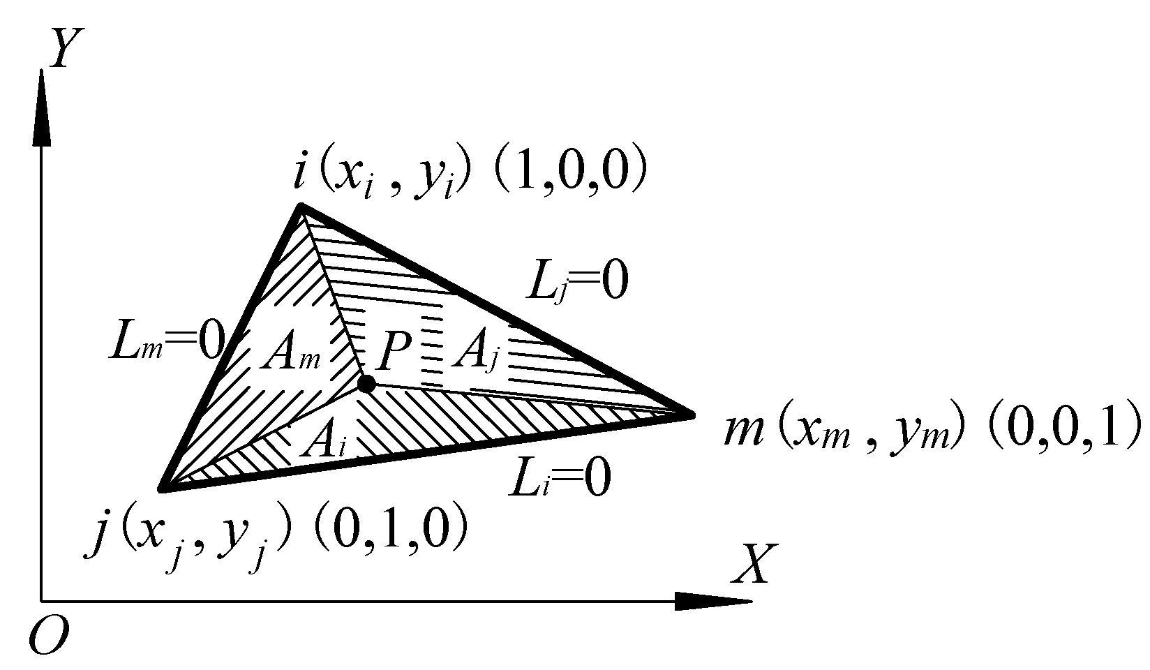
In Figure 3, three sub-triangles (Pjm, Pmi and Pij) are formed by connecting any point P in the triangle ijm with its three vertexes i, j and m.

Location of point P in the triangle ijm can be determined by either the Cartesian coordinate system O-XY or three sub-triangles. Areas of three sub-triangles (Pjm, Pmi and Pij) are ∆_Pjm, ∆_Pmi and ∆_Pij, respectively. The ratios between areas of three sub-triangles and the area of the triangle ijm (∆_Pjm/∆, ∆_Pmi/∆ and ∆_Pij/∆), can be expressed as $L_i$, $L_j$ and $L_m$:

$$\{\begin{array}{l}{L}_i=\frac{{\Delta }_{Pjm}}{\Delta }=\frac{{\Delta }_i}{\Delta }\\ L_j=\frac{{\Delta }_{Pmi}}{\Delta }=\frac{{\Delta }_j}{\Delta }\\ L_m=\frac{{\Delta }_{Pij}}{\Delta }=\frac{{\Delta }_m}{\Delta }\end{array}$$

(3)

L_i, L_j and L_m are area coordinate values of P. In Figure 3, the area coordinate value of any point on relative sides of each vertex of the triangle is 0. Generally, the relationship between area coordinate values is:

$$L_i+L_j+L_m=1$$

(4)

The mapping relation of P from O-XY to the area coordinate system is:

$$\left\{\begin{array}{c}{L}_i\\ L_j\\ L_m\end{array}\right\}=\frac{1}{2\Delta }\left[\begin{array}{ccc}{a}_i& b_i& c_i\\ a_j& b_j& c_j\\ a_m& b_m& c_m\end{array}\right]\left\{\begin{array}{c}1\\ x\\ y\end{array}\right\}$$

(5)

where a_i, b_i, c_i, a_j, b_j, c_j, a_m, b_m and c_m are algebraic cofactor of elements in the first, second and third rows at the right determinant of the calculation formula of triangle in Equation (6):

$$2\Delta =\left|\begin{array}{ccc}1& x_i& y_i\\ 1& x_j& y_j\\ 1& x_m& y_m\end{array}\right|$$

(6)

According to properties of the determinant and Equation (4), the mapping relation of P from O-XY to the area coordinate system is:

$$\left\{\begin{array}{c}1\\ x\\ y\end{array}\right\}=\left[\begin{array}{ccc}1& 1& 1\\ x_i& x{}_j& x_m\\ y_i& y_j& y_m\end{array}\right]\left\{\begin{array}{c}{L}_i\\ L_j\\ L_m\end{array}\right\}$$

(7)

It can be known from Equations (5) and (7) that locations of P in O-XY correspond to ∆_Pjm, ∆_Pmi and ∆_Pij.

3.2. Area Coordinate System Based on Axis DOFs

Equation (7) is equivalent to expressing the Cartesian coordinates of points in the triangle by coordinate interpolation of triangle vertexes. Since axis TF in the cylinder tolerance zone has four DOFs, interpolation of the ultimate state on each DOF can be used to express axis pose.

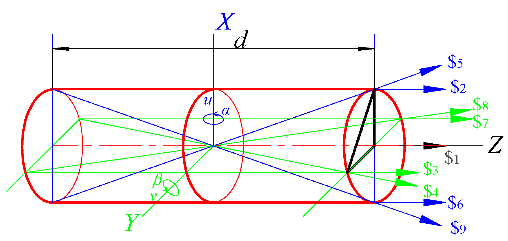
The cylinder tolerance zone in Figure 1 is extracted and amplified to Figure 4. Base lines $₂ and $₃ in Figure 4 are pose of axis TF when the translational displacement along X and Y axes in O-XYZ are at the maximum. Under this circumstance, the corresponding area coordinate values λ₂ and λ₃ are equal to 1. Their contribution to axis variation on the translational DOF are u and v. Base lines $₄ and $₅ are the pose of axis TF when the rotations around X and Y axes in O-XYZ are at the maximum. At this time, the corresponding area coordinate values λ₄ and λ₅ are equal to 1. Their contributions to axis rotation on the rotational DOF are α and β. $₁ is pose of axis TF when there is no error. $ is the axis of any pose in the tolerance zone and can be expressed by linear Equation (8) [19].

$ = λ₁$₁ + λ₂$₂ + λ₃$₃ + λ₄$₄ + λ₅$₅

(8)

Equation (8) reflects that any pose of axis TF correspond to one point in the four-dimensional space in the area coordinate value (λ₁, λ₂, λ₃, λ₄, λ₅). In other words, any axis pose in the tolerance zone in Figure 1 can establish linear relationships with tolerance and clearance through Equation (8). Here, (λ₁, λ₂, λ₃, λ₄, λ₅) might be negative and is used to express situations when variables u_i, v_i, α_i and β_i are negative. Therefore, with reference to Equation (4), the constraint relation between area coordinate values of axis TF can be improved as:

$$\left|{\lambda }_1\right|+\left|{\lambda }_2\right|+\left|{\lambda }_3\right|+\left|{\lambda }_4\right|+\left|{\lambda }_5\right|=1$$

(9)

For instance, $₁ expresses the ideal location of axis and (λ₁, λ₂, λ₃, λ₄, λ₅) = (1, 0, 0, 0, 0). When the axis is at $₄, (λ₁, λ₂, λ₃, λ₄, λ₅) = (0, 0, 0, 1, 0). When the axis is at $₇, (λ₁, λ₂, λ₃, λ₄, λ₅) = (0, 0, −1, 0, 0). This constraint relation ensures the coordinated relations among ultimate errors of axis TF on multiple DOFs.

4. Pose Decoupling of Axis TF

Research of robotics and its associated mechanisms, including location recognition of the mechanisms, kinematic control and dynamic simulation, all require pose decoupling analysis of the mechanism first [20,21]. Since TF in the tolerance zone has strong coupling, performance evaluation and analysis of assembly systems during the product design stage needs pose decoupling of TF of uncertainty error.

The process of establishing the functional relationship of the tolerance value and clearance value with the TF pose is known as TF decoupling.

4.1. Plücker Coordinates of Axis TF

Axis TF is determined by two end points on two end faces of the tolerance zone. Under this circumstance, Plücker coordinates of the straight line are introduced in order to describe its pose [22]. In Figure 2, the points of intersection that the axis passes through the two end faces of the cylinder tolerance zone are $S_1\left(x_1,y_1,-\frac{d}{2}\right)$ and $S_2\left(x_2,y_2,\frac{d}{2}\right)$, thus getting the Grassmann determinant of axis TF:

$$\left|\begin{array}{cccc}1& x_1& y_1& -\frac{d}{2}\\ 1& x_2& y_2& \frac{d}{2}\end{array}\right|$$

(10)

According to Plücker [22], coordinate values (L, M, N; P, Q, R) of the axis correspond to 6 of 2 × 2 determinants:

$$L=\left|\begin{array}{cc}1& x_1\\ 1& x_2\end{array}\right|, M=\left|\begin{array}{cc}1& y_1\\ 1& y_2\end{array}\right|, N=|\begin{array}{cc}1& -\frac{d}{2}\\ 1& \frac{d}{2}\end{array}|, P=\left|\begin{array}{cc}{y}_1& -\frac{d}{2}\\ y_2& \frac{d}{2}\end{array}\right|, Q=\left|\begin{array}{cc}-\frac{d}{2}& x_1\\ \frac{d}{2}& x_2\end{array}\right|, R=\left|\begin{array}{cc}{x}_1& y_1\\ x_2& y_2\end{array}\right|$$

(11)

(L, M, N; P, Q, R) is the pose of the axis in the tolerance domain, where L, M and N are direction ratios of the axis, P, Q and R are moments of line of unit force on the axis, relative to the origin O. It can be seen from Equation (11) that N = d is a zero-order constant. L, M, P and Q are first-order small quantities with the same magnitude of tolerance [t], while R is the high-order small quantity of [t]² level. Therefore, R can be omitted [19].

Base lines $₁, $₂, $₃, $₄ and $₅ in Figure 4 are ultimate locations on DOF when the axis is in the tolerance zone. Therefore, Plücker coordinates of each base line in the tolerance zone can be expressed as forms of matrix [X]. It can be seen from Equation (12), that the ith column in [X] is the Plücker coordinate of $_i (i = 1 to ~5).

$$\left[X\right]=\left[\begin{array}{ccccc}0& 0& 0& t& 0\\ 0& 0& 0& 0& t\\ d& d& d& d& d\\ 0& 0& \frac{t}{2}d& 0& 0\\ 0& -\frac{t}{2}d& 0& 0& 0\end{array}\right]$$

(12)

4.2. Mapping between the Area Coordinate System and Cartesian Coordinate System

For axis TF with any pose, Equation (8) can be expressed by a linear matrix:

$$\left[\begin{array}{c}L\\ M\\ N\\ P\\ Q\end{array}\right]=\left[X\right]\left[\begin{array}{c}{\lambda }_1\\ {\lambda }_2\\ {\lambda }_3\\ {\lambda }_4\\ {\lambda }_5\end{array}\right]$$

(13)

Combining Equations (11)–(13), the axis of any pose in the tolerance zone can be expressed by either Plücker coordinates in the Cartesian coordinate system directly, or the linear sum of Plücker coordinates of five base lines in the area coordinate system. These two expressions are equivalent:

$$\left[\begin{array}{c}L\\ M\\ N\\ P\\ Q\end{array}\right]=\left[\begin{array}{c}t{\lambda }_4\\ t{\lambda }_5\\ d\left({\lambda }_1+{\lambda }_2+{\lambda }_3+{\lambda }_4+{\lambda }_5\right)\\ \frac{t}{2}d{\lambda }_3\\ -\frac{t}{2}d{\lambda }_2\end{array}\right]$$

(14)

By solving the Equation (14), the S₁(x₁,y₁,−d/2) and S₂(x₂,y₂,d/2) which are coordinate values of S₁ and S₂ in the expression of area coordinate values (λ₁, λ₂, λ₃, λ₄, λ₅) can be obtained:

$$\left[\begin{array}{c}{x}_1\\ y_1\\ x_2\\ y_2\end{array}\right]=\left[\begin{array}{c}\frac{t}{2}\left({\lambda }_2-{\lambda }_4\right)\\ \frac{t}{2}\left({\lambda }_3-{\lambda }_5\right)\\ \frac{t}{2}\left({\lambda }_2+{\lambda }_4\right)\\ \frac{t}{2}\left({\lambda }_3+{\lambda }_5\right)\end{array}\right]$$

(15)

Similarly, the error transformation matrix can be expressed by area coordinate values (λ₁, λ₂, λ₃, λ₄, λ₅). It can be seen from Figure 2 that variables on four DOFs can be expressed by the area coordinate system:

$$\{\begin{array}{c}{u}_i=\frac{t}{2}{\lambda }_2\\ v_i=\frac{t}{2}{\lambda }_3\\ {\alpha }_i=-\frac{t}{d}{\lambda }_4\\ {\beta }_i=\frac{t}{d}{\lambda }_5\end{array}$$

(16)

By bringing Equation (16) into Equation (2), the error transformation matrix which is expressed by the area coordinate system can be obtained.

The analytic expression of error propagation which is expressed by area coordinate values can be gained from the tolerance analysis method based on the tracking local coordinate system [19]. Since (λ₁, λ₂, λ₃, λ₄, λ₅) range from −1 to 1, any pose of axis TF in the tolerance zone can be decoupled by changing (λ₁, λ₂, λ₃, λ₄, λ₅).

When calculating the limits of target feature variations, basic area coordinate values (each row) of the base line in the matrix (17) are permutated and combined, and then brought into the tolerance analysis model, so the analytic expression of the convex hull model which reflects variations in the target feature, can be found.

$$\left[\begin{array}{l}\left\{\begin{array}{ccccc}{\lambda }_1& {\lambda }_2& {\lambda }_3& {\lambda }_4& {\lambda }_5\end{array}\right\}\\ \begin{array}{ccccc}-1& 0& 0& 0& 0\\ 0& -1& 0& 0& 0\\ 0& 0& -1& 0& 0\\ 0& 0& 0& -1& 0\\ 0& 0& 0& 0& -1\\ 0& 0& 0& 0& 1\\ 0& 0& 0& 1& 0\\ 0& 0& 1& 0& 0\\ 0& 1& 0& 0& 0\\ 1& 0& 0& 0& 0\end{array}\end{array}\right]$$

(17)

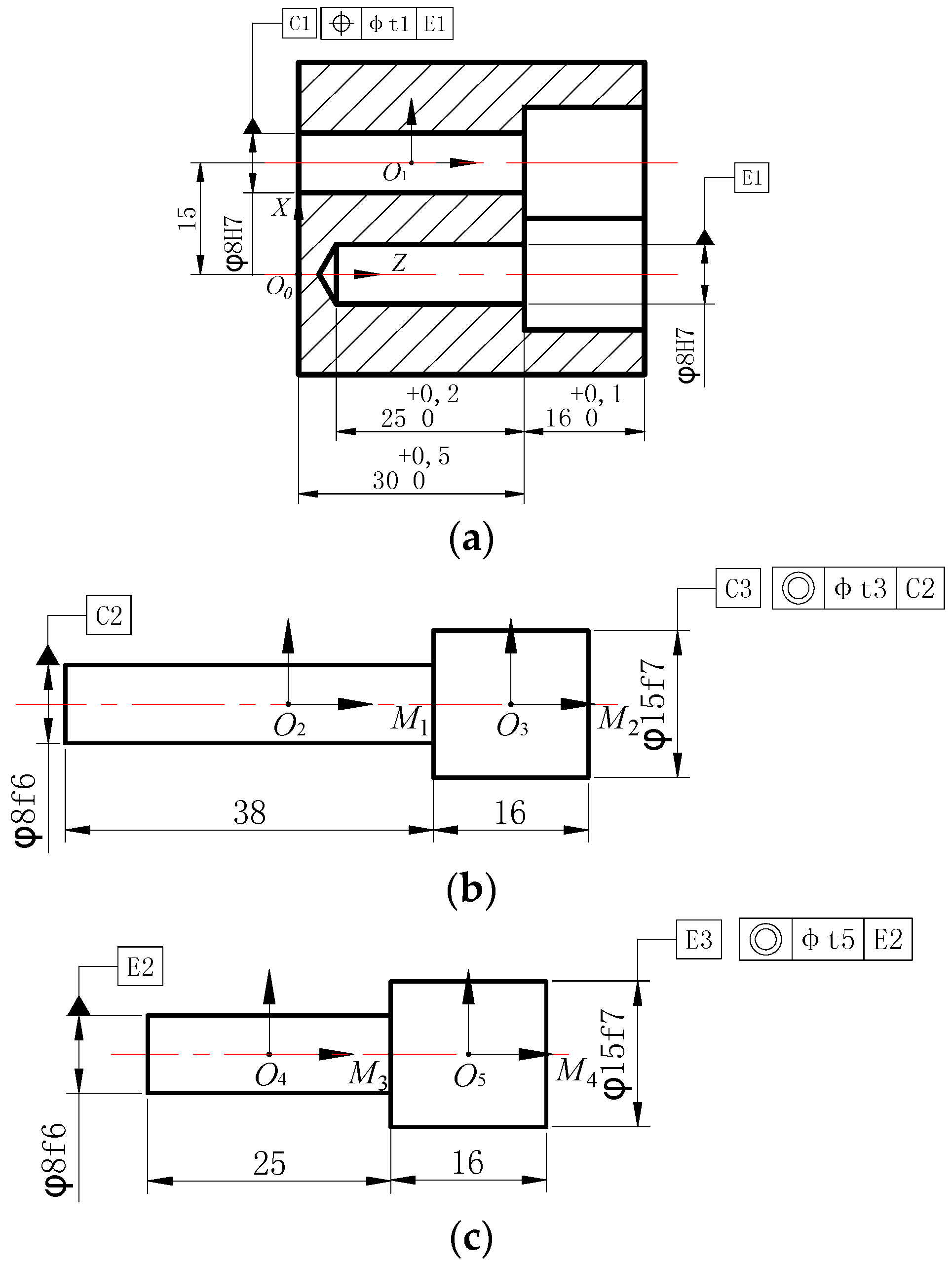
5. Case Study

The gear pump [9,23] in Figure 5 is composed of (a) pump body, (b) leading shaft and gear, and (c) shaft and gear. The gear is made of 45^# steel. The number of teeth is z = 10 and the number of modules is m = 1.5. Rated pressure is 25 Mpa and rated speed is 1450 r/min. The proportional factor of temperature deviation is 1. In the following text, the proposed model is used for pose decoupling analysis of the gear axis.

In Figure 5, local coordinate systems are constructed at TF of each part. Since the nominal coordinate system is very close to the tracking local coordinate system and actual local coordinate system, only the nominal coordinate system is expressed [19]. Through analysis, this gear pump can construct two open-looped dimension chains which have a consistent starting point. The starting point of two open-looped dimension chains is in the origin of the reference coordinate system, O₀ in Figure 5.

Dimension chain 1 included three links: tolerance feature C1 (corresponding to position tolerance t1), tolerance features C1 & C2 (corresponding to clearance fit tolerance t2) and C3 (corresponding to coaxiality tolerance t2), while dimension chain 2 only included two links: tolerance features E1 & E2 (corresponding to gap fit tolerance t4) and E3 (corresponding to coaxiality tolerance t5). Tolerance and the type of TF of dimension chain 2 could be found in dimension chain 1 which was more complicated with greater representativeness. Therefore, only dimension chain 1 was selected for explanation.

Dimension chain 1 is formed by connecting nominal coordinate systems O₀, O₁, O₂ and O₃, whereas dimension chain 2 is formed by connecting nominal coordinate systems O₀, O₄ and O₅. Here, the dimension chain 1 was used as the example. Transformation among the nominal local coordinate systems (T₁) is:

$${\mathit{T}}_{\mathbf{1}}=P_{{\mathit{O}}_{\mathbf{1}}\to {\mathit{O}}_{\mathbf{0}}}{\mathit{D}}_{\mathbf{1}}{\mathit{P}}_{{\mathit{O}}_{\mathbf{2}}\to {\mathit{O}}_{\mathbf{1}}}{\mathit{D}}_{\mathbf{2}}{\mathit{P}}_{{\mathit{O}}_{\mathbf{3}}\to {\mathit{O}}_{\mathbf{2}}}{\mathit{D}}_{\mathbf{3}}$$

(18)

The homogeneous coordinate value of end point, M₁ in the nominal local coordinate system, O₃ is ${\left[{\mathbf{M}}_1\right]}_{O_3}={\left(0,0,-8,1\right)}^T$. Then, the coordinate value in the reference coordinate system O₀ is [M₁]_O0:

$${\left[{\mathit{M}}_{\mathbf{1}}\right]}_{O_0}={\mathit{T}}_{\mathbf{1}}{\left[{\mathit{M}}_{\mathbf{1}}\right]}_{O_3}$$

(19)

Combined with Equation (16), [M₁]_O0 which is expressed by the area coordinate value can be obtained:

$${\left[{\mathbf{M}}_{\mathbf{1}}\right]}_{O_0}=\left[\begin{array}{l}\frac{{\lambda }_{2\_1}{t}_1+{\lambda }_{2\_2}{t}_2+{\lambda }_{2\_3}{t}_3}{2}+\frac{15{\lambda }_{5\_1}{t}_1+15{\lambda }_{5\_2}{t}_2}{d_1}-\frac{8{\lambda }_{5\_3}{t}_3}{d_3}+15\\ \frac{{\lambda }_{3\_1}{t}_1+{\lambda }_{3\_2}{t}_2+{\lambda }_{3\_3}{t}_3}{2}-\frac{15{\lambda }_{4\_1}{t}_1+15{\lambda }_{4\_2}{t}_2}{d_1}\\ \frac{8{\lambda }_{5\_3}{t}_3\left({\lambda }_{5\_1}{t}_1+{\lambda }_{5\_2}{t}_2\right)}{d_1{d}_3}+30\end{array}\right]$$

(20)

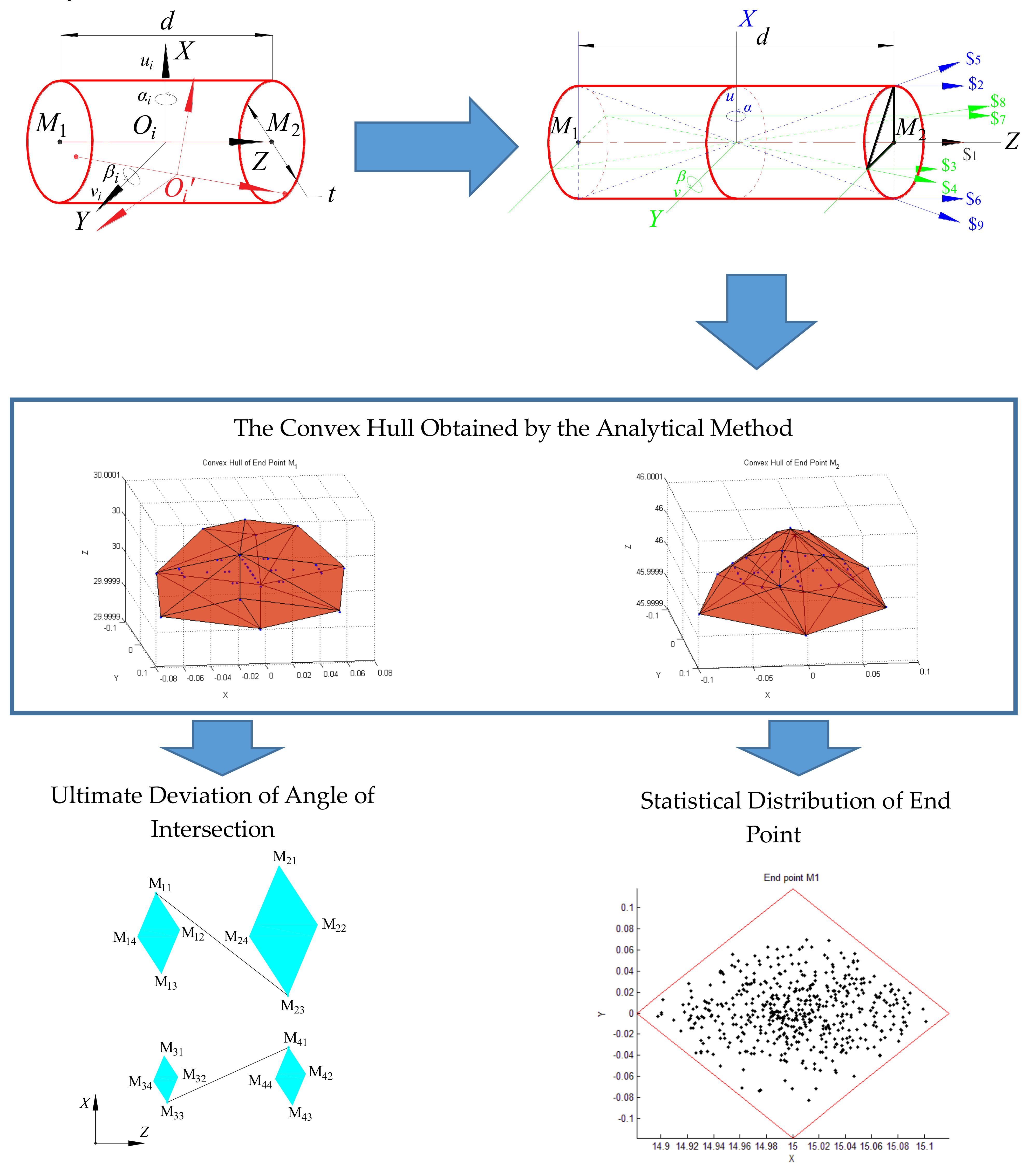
Equation (20) not only establishes relationships between any pose of point M₁ and the tolerance value and clearance value, but it can also find the limits of target feature variations when λ_i = ±1 (i = 1~5), that is, the vertex of the convex hull. After calculation, permutation and combination of basic area coordinate values in Equation (17) are brought into Equation (20), then the three-dimensional scatter points in Euclidean space can be acquired. Each scatter point represents one possible limit value. Next, using MATLAB (R2012b, MathWorks, Natick, MA, USA), the smallest convex hull model which covers all scatter points is searched for Vertexes of the convex hull are the pose limits of point M₁. Convex hulls concerning variations of point M₁ and point M₂, as well as their projection on three coordinate planes of the reference coordinate system, O₀ are listed in

Table 1. Envelope diagram concerning variations of end point M₁ and M₂ of the leading shaft.

The Type of Convex Hull	End Point M1	End Point M2
Three-diminsional convex hull
Plane XOY
Plane YOZ
Plane XOZ

.

Similarly, convex hulls of end point M₃ and M₄ variations, as well as their projections on three coordinate planes of the reference coordinate system, O₀ are listed in

Table 2. Envelope diagram concerning variations of end point M₃ and M₄ of shaft and gear axis.

The Type of Convex Hull	End Point M3	End Point M4
Three-diminsional convex hull
Plane XOY
Plane YOZ
Plane XOZ

.

Accurate coordinate values for the variation range of end points of the gear axis with consideration to deviations can be gained from Table 1 and Table 2. They are listed in

Table 3. Variation ranges of four end points of the gear axis (Unit: mm).

End Point	Variation Range of X Axis	Variation Range of Y Axis	Variation Range of Z Axis
Point M1	(14.8815, 15.1185)	(−0.1185, 0.1185)	(29.99971, 30.00023)
Point M2	(14.8084, 15.1916)	(−0.1916, 0.1916)	(45.9996, 46.0002)
Point M3	(−0.0685, 0.0685)	(−0.0685, 0.0685)	(29.99993, 30.00006)
Point M4	(−0.08515, 0.08515)	(−0.08515, 0.08515)	(45.99994, 46.00006)

. Therefore, accurate pose of the gear axis with different ultimate deviations could be acquired, thus enabling simulation analysis on the performance of the gear pump with consideration of deviation. Table 3 reveals that the maximum magnitude of deviation along Z direction is 10⁻⁴ and the magnitude along X and Y directions ranges from 10⁻¹ to ~10⁻². Generally, deviation along the Z direction can be neglected.

For gear pump (see Figure 5), gear engagement performance can significantly influence the flow rate of the gear pump. The parallel misalignment, deviation of the angle of intersection and deviation of the angle of stagger between M₁M₂ and M₃M₄ will influence gear engagement, thus affecting the service ability of the gear pump. Therefore, all accumulated errors on dimension chain 1 and dimension chain 2 can be concentrated into the gear axis during performance simulation of the gear pump. This is demonstrated by taking the angle of intersection, for example.

According to the definition of an intersection angle, it can easily be seen from the second row of Table 1 and Table 2, that the extreme value of the error in the angle intersection is 1.6604°. As the deviation along the Z axis is neglected, the error is a combined effect of deviations at two DOFs, namely, translation along the X axis and rotation around the Y axis. Ultimate pose combinations of two gear axes are M₁₁M₂₃ + M₃₃M₄₁ and M₁₃M₂₁ + M₃₁M₄₃, respectively. Since the tolerance zone is symmetric in this case, the ultimate angles of interaction which is gained from the combination of two groups of poses are equal in numerical value and opposite in direction. Therefore, calculating the angle of intersection of one combination is enough. In the following analysis, M₁₁M₂₃ + M₃₃M₄₁ is chosen. Accumulative errors of the two dimension chains are converted to local coordinate systems O₃ and O₅, so translation deviations of M₁M₂ and M₃M₄ in dimension chains 1 and 2 along the X axis are u_{3_C1} and u_{5_C2}, and the rotation deviations around the Y axis are β_{3_C1} and β_{5_C2}. Specific data are listed in

Table 4. Ultimate deviation of angle of intersection and pose expression of gear axis.

	Ultimate Deviation of Gear Axis	M1M2	M3M4
	$u_{3\_C1}$	−0.03655 mm
	${\beta }_{3\_C1}$	−0.01938°
	$u_{5\_C2}$		0.008325 mm
	${\beta }_{5\_C2}$		0.009603°

. It only remains to bring these data into gear engagement analysis with the ultimate deviation of angle of intersection. Similarly, the translation deviation and rotation deviation of M₁₃M₂₁ + M₃₁M₄₃ could be acquired.

Therefore, the accurate ultimate deviation of the angle of intersection can be obtained through pose decoupling of the gear axis. Similarly, the pose combinations of ultimate parallel misalignment between two gear axes are M₁₁M₂₁ + M₃₃M₄₃ and M₁₃M₂₃ + M₃₁M₄₁, and the pose combinations of ultimate angle deviation of stagger are M₁₂M₂₄ + M₃₄M₄₂ and M₁₄M₂₂ + M₃₂M₄₄, respectively. Accurate deviations on corresponding DOF can be gained in the same way as the angle of interaction.

This decoupling model is also applicable to statistical analysis. It is already known that area coordinate values of TF_i meet constraint relation as shown in Formula (9), based on which area coordinate values ${\lambda }_{2\_1}$, ${\lambda }_{3\_1}$, ${\lambda }_{4\_1}$, ${\lambda }_{5\_1}$; ${\lambda }_{2\_2}$, ${\lambda }_{3\_2}$, ${\lambda }_{4\_2}$, ${\lambda }_{5\_2}$; ${\lambda }_{2\_3}$, ${\lambda }_{3\_3}$, ${\lambda }_{5\_3}$ in Formula (20) can be given through sampling method in statistics. Through multiple simulations in Formula (20), namely Monte Carlo simulation, the distribution diagram of four end points M₁, M₂, M₃ and M₄ of gear axis can be obtained in

Table 5. Statistical distribution of end points of the gear axis.

Statistical distribution of end points of gear axis (simulation times N = 500)

.

The error value of each TF in the corresponding dimension chain can be found for each point in in Table 5. The error value can be the input data in the analysis of product performance.

6. Conclusions

Based on the widely-used shaft-hole fit, a decoupling model of axis TF in the cylinder tolerance zone was proposed based on an area coordinate system. By combining the improved tolerance analysis model based on tracking the local coordinate system, this model not only obtains expression of pose decoupling analysis on the dimension chain, but also visually displays the limits of target feature variations through a convex hull model. That is, the proposed model lays the foundation for product performance evaluation of axis TF assembly systems with any error.

References

- Akhadkar, N.; Acary, V.; Brogliato, B. 3D revolute joint with clearance in multibody systems. In Computational Kinematics; Springer: Cham, Switzerland, 2018; pp. 11–18. [Google Scholar]
- Aschenbrenner, A.; Wartzack, S. A Concept for the Consideration of Dimensional and Geometrical Deviations in the Evaluation of the Internal Clearance of Roller Bearings. Procedia CIRP 2016, 43, 256–261. [Google Scholar] [CrossRef]
- Liu, C.; Zhang, K.; Yang, R. The FEM analysis and approximate model for cylindrical joints with clearances. Mech. Mach. Theory 2007, 42, 183–197. [Google Scholar] [CrossRef]
- Warda, B.; Chudzik, A. Effect of ring misalignment on the fatigue life of the radial cylindrical roller bearing. Int. J. Mech. Sci. 2016, 111–112, 1–11. [Google Scholar] [CrossRef]
- Wittwer, J.; Chase, K.; Howell, L. The direct linearization method applied to position error in kinematic linkages. Mech. Mach. Theory 2004, 39, 681–693. [Google Scholar] [CrossRef]
- Marziale, M.; Polini, W. A review of two models for tolerance analysis of an assembly: Vector loop and matrix. Int. J. Adv. Manuf. Technol. 2009, 43, 1106–1123. [Google Scholar] [CrossRef]
- Desrochers, A.; Ghie, W.; Laperriere, L. Application of a Unified Jacobian—Torsor Model for Tolerance Analysis. J. Comput. Inf. Sci. Eng. 2003, 3, 2–14. [Google Scholar] [CrossRef]
- Asante, J. A small displacement torsor model for tolerance analysis in a workpiece-fixture assembly. Proc. Inst. Mech. Eng. Part B J. Eng. Manuf. 2009, 223, 1005–1020. [Google Scholar] [CrossRef]
- Desrochers, A.; Rivière, A. A matrix approach to the representation of tolerance zones and clearances. Int. J. Adv. Manuf. Technol. 1997, 13, 630–636. [Google Scholar] [CrossRef]
- Whitney, D.; Gilbert, O.; Jastrzebski, M. Representation of geometric variations using matrix transforms for statistical tolerance analysis in assemblies. Res. Eng. Des. 1994, 16, 191–210. [Google Scholar] [CrossRef]
- Parenti-Castelli, V.; Venanzi, S. Clearance influence analysis on mechanisms. Mech. Mach. Theory 2005, 40, 1316–1329. [Google Scholar] [CrossRef]
- Schleich, B.; Wartzack, S. How to determine the influence of geometric deviations on elastic deformations and the structural performance? Proc. Inst. Mech. Eng. Part B J. Eng. Manuf. 2013, 227, 754–764. [Google Scholar] [CrossRef]
- Marques, F.; Isaac, F.; Dourado, N. An enhanced formulation to model spatial revolute joints with radial and axial clearances. Mech. Mach. Theory 2017, 116, 123–144. [Google Scholar] [CrossRef]
- Fernández, A.; Iglesias, M.; De-Juan, A. Gear transmission dynamic: Effects of tooth profile deviations and support flexibility. Appl. Acoust. 2014, 77, 138–149. [Google Scholar] [CrossRef]
- Giordano, M.; Pairel, E.; Samper, S. Mathematical Representation of Tolerance Zones; Springer: Dordrecht, The Netherlands, 1999; pp. 177–186. [Google Scholar]
- Mujezinović, A.; Davidson, J. A New Mathematical Model for Geometric Tolerances as Applied to Polygonal Faces. J. Mech. Des. 2003, 126, 504–518. [Google Scholar] [CrossRef]
- Giordano, M.; Samper, S.; Petit, J. Tolerance Analysis and Synthesis by Means of Deviation Domains, Axi-Symmetric Cases; Springer: Dordrecht, The Netherlands, 2007; pp. 85–94. [Google Scholar]
- Zhai, X.; Du, Q.; Wang, W. A new approach to tolerance analysis based on tracking local coordinate systems. J. Adv. Mech. Des. Syst. Manuf. 2017, 11, 1–8. [Google Scholar] [CrossRef]
- Bhide, S.; Davidson, J.; Shah, J. A New Mathematical Model for Geometric Tolerances as Applied to Axes. Proceedings of ASME 2003 Design Engineering Technical Conferences and Computers and Information in Engineering Conference (DETC’03), Chicago, IL, USA, 2–6 September 2003; pp. 1–9. [Google Scholar]
- Jin, Y.; Chen, I.; Yang, G. Kinematic design of a 6-DOF parallel manipulator with decoupled translation and rotation. IEEE Trans. Robot. 2006, 22, 545–551. [Google Scholar] [CrossRef]
- Awtar, S.; Ustick, J.; Sen, S. An XYZ Parallel Kinematic Flexure Mechanism with Geometrically Decoupled Degrees of Freedom. In Proceedings of the ASME 2011 International Design Engineering Technical Conferences and Computers and Information in Engineering Conference, Washington, DC, USA, 28–31 August 2011; pp. 119–126. [Google Scholar]
- Dai, J. Geometrical Foundations and Screw Algebra for Mechanisms and Robotics; Higher Education Press: Beijing, China, 2014. [Google Scholar]
- Li, P.; Zhang, W.; Chen, C. Prediction of Operating Loads Contribution to Assembly Relation and Product Behavior. J. Softw. 2009, 1, 11–18. [Google Scholar] [CrossRef]
Figure 1.
Shaft-hole fit and cylinder tolerance zone.
Figure 2.
Variation of axis tolerance features (TF) in cylinder tolerance zone.
Figure 3.
Area coordinate system of triangles.
Figure 4.
Cylinder tolerance zone and baselines of area coordinate system corresponding to axis TF.
Figure 5.
Gear pump (Unit:mm): (a) Pump body; (b) Leading shaft and gear; (c) Shaft and gear.