Abstract
Nowadays, simultaneous localization and mapping (SLAM) algorithms support several commercial sensors which have recently been introduced to the market, and, like the more common mobile mapping systems (MMSs), are designed to acquire three-dimensional and high-resolution point clouds. The new systems are said to work both in external and internal environments, and completely avoid the use of targets and control points. The possibility of increasing productivity in three-dimensional digitization projects is fascinating, but data quality needs to be carefully evaluated to define appropriate fields of application. The paper presents the analytical measurement principle of these indoor mobile mapping systems (IMMSs) and the results of some tests performed on three commercial systems. A common test field was defined in order to acquire comparable data. By taking the already available terrestrial laser scan survey as the ground truth, the datasets under examination were compared with the reference and some assessments are presented which consider both quantitative and qualitative aspects. Geometric deformation in the final models was computed using the so-called Multiscale Model to Model Cloud Comparison (M3C2) algorithm. Cross sections and cloud to mesh (C2M) distances were also employed for a more detailed analysis. The real usability assessment is based on the features of recognizability, double surface evidence, and visualization effectiveness. For these evaluations, comparative images and tables are presented.
1. Introduction
In the geomatics community, the technical requirements and resulting potentialities of the terrestrial surveying of objects of interest (buildings, cultural heritage, civil structures, industrial environments, etc.) are well known. In addition, it is also widely known how these activities are carried out nowadays, that is, by means of terrestrial laser scanning (TLS) and/or photogrammetric images, whose somewhat complementary features are compared by the authors of [1].
In TLS surveying, the scanner instrument is placed on a tripod in a sequence of static scan stations in order to survey “all” of the surfaces to be measured, that is, the inside and outside of an element of architecture. These various scans are later registered together, generally by using many artificial targets placed over the scanned object as tie points. It is better if they are surveyed by a total station in order to acquire control points and ensure, after the classical least square adjustment of the topographic measurements, the best geo-referencing of the whole obtained point cloud.
On the other hand, photogrammetric surveying uses many digital images which are frequently acquired these days by means of uncalibrated cameras. The interior and exterior image orientation process is resolved by automatic procedures developed in the computer vision community, following an approach known as “structure from motion” (SfM). This last expression derives from the fact that the photographed object (structure) is surveyed by estimating the position and rotation (motion) of the imaging sensor, which is computed in a single automatic step (apart from the scale factor of the model). Although the term “motion” is contained in this approach, and the images really can be acquired by a moving charge-coupled device CCD (for instance, mounted on/inside a drone), the analytical solution considers each image to be statically acquired, and the control points have the same role as in TLS surveying (and are essential for the estimation of the model scale factor).
The necessity to have known control points is instead overcome once and for all with indoor mobile mapping systems (IMMSs) (e.g., in [2]), a new form of surveying technology developed in recent years. These systems are also referred to as human (e.g., in [3]), handheld (e.g., in [4]), backpack (wearable) (e.g., in [5]), portable (e.g., in [6]), or trolley (e.g., in [7]) (mapping) systems in the literature. Within the cited references, not only are many instrumental details and configuration differences found, but important theoretical issues regarding the complex analytical models are also addressed. Nevertheless, all of these systems perform the surveying in a similar way, using a linear scanner as the measurement sensor, although some instead make use of imaging or range cameras. In other words, an IMMS is a moving multi-sensor system which surveys the surrounding environment in a kinematic manner.
From the geomatics point of view, IMMSs are very similar to the mobile mapping systems (MMSs) devised for road cadastres more than 20 years ago [8]. At that time, these vehicles, usually vans, were developed with photogrammetric imaging sensors, while nowadays they are used with more advanced surveying devices to quickly capture the geometry of a road (and the buffer area around it) thanks to a global navigation satellite system (GNSS) receiver and an inertial navigation system (INS) platform mounted onto the vehicle [9]. Some analytical details on the MMS surveying principle are explained in Section 2.1, but it is evident that GNSS/INS navigation sensors enable an estimation of the position and the attitude of the vehicle, and then of the CCD or the video-camera, in each instant. The revolution introduced by MMSs was the direct orientation of the imaging sensors thanks to the navigation sensors, thus avoiding the classical indirect method which instead used control points and required topographical surveys.
The term “indoor” differentiates IMMSs from MMSs. However, the former are not for exclusive indoor use since outdoor applications can be also carried out with IMMSs. The situations in which GNSS data are not available urge a different approach to be used in solving the problem of instantaneous navigation. The analytical methods used to solve this chicken-or-egg problem often belong to the class of so-called “simultaneous localization and mapping” (SLAM) algorithms, originally developed in robotics. “Localization” involves the estimation of the position and attitude of a (measuring) sensor with respect to a certain coordinate system, while “mapping”, the obvious fundamental goal of any geomatics technique, is intended as the final output from the sensor, generally in the form of a digital representation of the surveyed environment. To sum up, with a SLAM algorithm it is possible to simultaneously build a map and localize the sensor within the map: obviously the essential aim is the mapping (for the surveyors’, not the robotics community), but the localization problem is also solved, almost in real time.
In the last few years, the number of IMMSs put on the geomatics market has increased greatly, with a fairly diversified range of solutions: the aim of this paper is to evaluate the potentials and limitations of three different systems commercialized in Italy over a diversified test field, characterized by the widest possible variety of conditions (indoor, outdoor, different elevations, stairs, wide and narrow spaces, trees, moving objects) in order to adequately reproduce very general surveying situations. As detailed further on, the point clouds acquired by a traditional static TLS were considered as reference values, that is, the so-called “ground truth” for testing these IMMSs.
Very interesting examples of IMMS comparisons are reported in [10,11,12]. In 2013, Thomson et al. [10] investigated two very different products: the Viametris i-MMS trolley without GNSS/INS sensors, and the handheld 3D Laser Mapping/CSIRO ZEB1, while taking indoor scans acquired by means of a Faro Focus 3D as a reference. Nocerino et al. [11] compare two similar systems, the handheld GeoSlam Zeb-Revo and the Leica Pegasus Backpack, the latter equipped with a GNSS receiver. One of the tests was performed inside a two-floor building scanned with a Leica HDS7000 and the other outdoors in a big (80 m × 70 m) city square, previously surveyed with a “classical” MMS, namely a Riegl VMX-450 mounted on a van. The comparison carried out by Lehtola et al. [12] is quite impressive since it makes a comparison of no fewer than eight different systems: five commercial ones—the innovative Matterport 3D camera, the NavVis trolley, the spring-mounted handheld Zebedee (the oldest Zeb model), the handheld Kaarta Stencil, and again the Leica Pegasus Backpack—and three interesting research prototypes—the Aalto VILMA “rotating wheel”, the FGI Slammer, and the Würzburg backpack. Furthermore, these systems were analysed in three test areas (however, in truth, not all of them were): a hallway and a car park with a sloping floor (with both sites surveyed by a Leica ScanStation P40), and an industrial hall set out as a co-working space, which was scanned with a Faro Focus 3D.
Of course, IMMS models can be compared with models from SfM-based photogrammetric surveying, while keeping statically acquired TLS data as a reference, as reported for example in [13].
In the examination proposed in this paper, the models analysed are the Kaarta Stencil, the Pegasus Leica Backpack, and the GeoSlam Zeb-Revo, while the reference is given by a Z+F TLS.
2. Materials and Methods
2.1. The IMMS Analytical Measurement Principle
As hinted in the Introduction, these days the IMMS is without doubt the most innovative terrestrial surveying technique, as it finely exploits the availability of more measuring sensors such as (at a minimum) a linear 2D or a 3D laser scanner, an inertial platform, and perhaps a satellite receiver.
As said earlier, from the analytical point of view, the IMMS measuring principle is analogous to the one proposed in 1996 by Schwarz and El-Sheimy [14] for MMSs: for IMMSs, by simply considering the six degrees of freedom of a laser scanning sensor instead of the imaging sensor and re-arranging the equation, the position of a generic i-th point with respect to a chosen global coordinate system (GCS) is given by the equation below:
where:
- is the position of the GNSS/INS sensors (sometimes embedded) in the GCS frame, computed in an integrated way as reported further on;
- is the rotation matrix from the INS frame to the GCS frame, with the instantaneous rotation angles measured by the three INS gyroscopes. Together with the three accelerometers, they form the so-called “inertial measurement unit” (IMU) [9];
- is the rotation matrix from the TLS frame to the INS frame, with fixed angles estimated in the IMMS system calibration procedure;
- is the rotation matrix from the instantaneous laser beam (b) to the TLS frame, with the variable angles imposed by the scanning system;
- is the laser beam on the i-th point;
- is the position of the TLS frame with respect to the INS frame, with fixed components (generally measuring a few centimetres) which must nevertheless be measured/estimated in the system calibration step.
The kinematic positioning of every scanned point by means of Equation (1) can be reinterpreted as the static positioning from a station whose instantaneous position and rotation enclosed in . That is, the six roto-translation registration parameters are estimated via GNSS/INS measurements and not by using tie points. From the analytical point of view, integrating GNSS and INS data is a very complex task [8,14], solved by means of Kalman filter-based procedures considering a “state vector” and using state equations (modelling the motion) and measurement equations (from the sensors). The INS-frame position and attitude are therefore continuously updated from an epoch t, when they are deemed to be known, to the following epoch t + 1, when they are instead unknown. As such, Equation (1) should also contain the term t, left out for the sake of simplicity, since all the quantities change over time, apart the from constant calibration terms and . Moreover, these quantities are observed with frequencies of different orders of magnitude: Hz for , hundreds of Hz for and , and tens of kHz for and . Hence, the synchronization of these observations becomes a fundamental hardware requirement and the timing interpolation has to be carried out correctly at the highest TLS frequency.
In addition to synchronization errors, each one of the above quantities is characterized by measurement errors, whose combined effect propagates onto the final positioning of the generic point. This error could be estimated by considering every independent contribution, as suggested for MMSs in [14], where they were evaluated at around 20 cm overall at a 30-m distance.
In any case, as is logical, error improves with the distance of the laser beam, in particular by taking into account the “level-arm” effect resulting from angular inaccuracies in the rotation matrix : since the main INSs used nowadays are micro-electromechanical systems (MEMS) with generally limited accuracy, this can produce very large errors in the positioning.
Special attention is also required in analysing the accuracy of the positioning obtained from the joint use of the satellite receiver and inertial platform, remembering that most applications of IMMS are in closed spaces and tunnels, where GNSS positioning is not available. In spite of this, supposing that both sensors are working, GNSS positioning becomes inaccurate when the available satellites are reduced by obstructions. Therefore, in such cases, the positioning can be estimated by INS accelerometers. The previously mentioned Kalman filter integration of the two navigation sensors allows one to augment and enhance the other: the absolute position (and also velocity) of the GNSS is used to compensate for the errors in the INS measurements, while the stable relative position of the INS is used to bridge over when the GNSS solution is of low quality or is unavailable.
To sum up, on one hand, the analytical principle expressed by Equation (1) can be considered as a new dynamic way of perceiving TLS surveying, while, on the other hand, it is an old idea from nearly 20 years ago in aerial laser scanning (ALS) methodology (e.g., [15]). In ALS, although could be kilometric with a speed of hundreds of km/h, the accuracy of the positioning is surprising, generally limiting the errors under to 10 cm.
If we are to recall the SLAM acronym, the novelty of the IMMS approach is that TLS sensor localization (position and rotation embedded in ), that is, the trajectory/orientation of the TLS system, and the mapping points (), that is, the 3D point cloud obtained, are considered as a “starting point” for the final solution. In this sense, the expression simultaneous localization (of the scanning sensor) and mapping (of the scanned points) is not exactly appropriate, since the simultaneity does not refer to a computational black box like in the SfM photogrammetric approach, where localization and mapping instead really are the output processes. Nevertheless, even if in truth IMMS provides the final cloud in two steps, the output model is so impressive that an extension of the term “simultaneous”, in the sense of being “automatic”, is due.
An important question instead concerns the contribution of the navigation GNSS/INS (navigation) sensors and the TLS and/or imaging (measuring) sensors to localization and mapping problems. In general, MMS technology uses the former for localization and the latter only for mapping: since navigation and measuring data have complementary strengths and weaknesses, a combination is instead advisable. We presented an example of such an integration [16] in 1998, using the images to solve the position and attitude estimation problem in a low-cost MMS system without INS sensors. On the other hand, nowadays photogrammetry carried out through a SfM approach generally only uses the images for localization and mapping. The originality of the IMMS principle is instead to take advantage of the mapped results to update the navigation results in order to consequently improve the mapped ones.
From the methodological point of view, the fundamental step is to make an appropriate subdivision of the whole point cloud into a lot of (n) “virtual single static scans”, with each one considering a certain TLS localization. Without doubt, such clouds have geometrical discrepancies due to the above-described errors: nevertheless, these are minimized by analytical procedures generally based on the well-known iterative closest point (ICP) algorithm, that is, by suitably reducing the distance between ideal surfaces from these n clouds.
A noteworthy SLAM/ICP procedure was proposed for robot relocalization in 2007 by Nuchter et al. [17]: in this article, the expression “6D SLAM”, or the more general “6DOF SLAM” reported in others, refers to the six degrees of freedom of the instantaneous TLS position and attitude. These values, also called “6D pose”, expressed in Equation (1) as position , and rotation angles embedded in , from now on will be rewritten as t and R as in [17]. The procedure consists of the next steps:
- Rough estimation of the six TLS degrees of freedom for any epoch, from the odometry data: this is always possible for a robot, while for an IMMS these estimations have to be made from INS data.
- Heuristic computations based on octree representation of the n scans and estimation of the best translation and rotation matching the couples of octrees, so as to improve the 6D poses given in step 1.
- Fine registration using the ICP approach for all n scans and not for only two scans as is customary; this is the crucial step in the procedure, in which the following cost (error) function has to be minimized [5,6]:in order to enable the calculation of the best and values for each scan on the base of tuples of corresponding points in an adequate overlapping area.
- If applicable, the closure of the loop of scans enables the distribution of the incremental residual error accumulated with the subsequent scans, that is, the first and last cloud do not correspond exactly: the computed ∆t and ∆R are distributed with a method similar to that used in the adjustment of closed polygonals.
- Final refinement of the whole model using a global relaxation method called “simultaneous matching”, which enables the residual alignment error to be diffused equally among the scans.
Of course, the systems on the market can implement SLAM/ICP procedures which may be different from the ones reported above, and the efficiency and robustness of the specific algorithm implemented in the processing software are nevertheless of great importance. On the other hand, although the positioning errors are strongly reduced by the SLAM/ICP procedures, recalling the application [14] of the error propagation law from Equation (1), the accuracy of the final IMMS cloud definitely depends on the instrumental accuracy, mainly of the TLS distance meter, but also of the INS accelerometers/gyroscopes and the GNSS receiver, especially when using low-cost sensors. By taking into account both software and hardware configurations, different IMMSs with similar sensors can deliver very dissimilar results in terms of correctness and accuracy.
Furthermore, even a trivial operational aspect such as the way the system is moved (slowly or quickly, above all when turned) influences the results: for instance, if the walking speed is halved, the cloud resolution, namely the points available for the ICP-based correction, is more or less doubled. Last but not least, despite operating exactly in the same instrumental/processing/acquisition conditions, the geometrical regularity and the surface material of the surveyed environment can locally affect the final accuracy. The space of a given geometry enclosed by smooth modern walls gives better results with respect to a historical one with irregular and decayed stones/bricks.
2.2. Technical Specifications of the Examined IMMSs
The three systems described later on (Kaarta Stencil, Leica Pegasus Backpack, and GeoSlam Zeb-Revo, shown in Figure 1) available for our test were all used by a walking operator in order to perform a correct comparison; for each one, various configurations on trolleys, bicycles, or cars could be also possible.
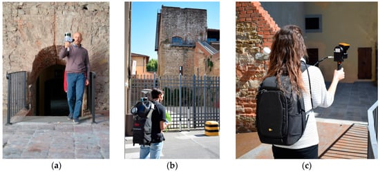
Figure 1.
The systems under testing during the field acquisitions: (a) Kaarta Stencil; (b) Leica Pegasus Backpack; (c) GeoSlam Zeb-Revo.
We consider the surveying data outputs, namely the final point clouds, as those provided to us by the system resellers: in one case (Kaarta Stencil) as directly downloaded from the instrument as soon as the measurements were made, and in the others as post-processed by them, also considering that post-processing software could require specialist knowledge and expertise. In this sense, we suppose that the datasets supplied to us are the best solution from each tested IMMS product, even though we are aware that many, and generally not comparable, software processing factors influence the cloud considered to be the final output.
2.2.1. Kaarta Stencil (Handheld)
The system [18] was tested on 19 September 2017.
The basic configuration (the one we tested) consists of an industrial PC, a Velodine VLP-16 linear scanner, a MEMS-based INS, and an industrial camera called “black and white” (in truth, acquiring 640 × 480 grey-scale images), mounted on a base with a standard photography thread size. A small tripod was used to support the system. The measurement principle of this system, conceived by Zhang and Singh from the Robotics Institute at Carnegie Mellon University [19], is different from the others considered in this study. It is called “Lidar Odometry And Mapping” (LOAM): by finely using two algorithms running in parallel, it allows a practically real-time solution. An odometry algorithm estimates the velocity of the TLS, therefore correcting the errors in the point cloud, while a mapping algorithm matches and registers the point cloud to create a map.
The Stencil is proposed commercially as a modular system, offering the opportunity to be configured with different sensors. It is possible to connect a tablet or a screen for real-time checks of the acquired data. New versions of the Stencil will be soon proposed, also including a GNSS receiver and/or a 360° panoramic camera for texturing purposes. Different mounting platforms can be used to scan from a backpack, a vehicle, or a drone. No accuracy specifications are available on the technical sheet [20]; a white paper [21] presents some accuracy tests by comparing the Stencil to static measurements with a Faro Focus 3D TLS.
In the tested configuration, the system was initially set up for use with the feature-tracking camera: this function is supposed to be helpful in scenes dominated by planar areas, like long and flat facades, tunnels, etc. The idea of using images for the localization problem, already mentioned in Section 2.1 for MMS, is proposed again by Zhang and Singh in [22], with “visual odometry” integrating the “lidar odometry” of [19]. Nevertheless, during the first acquisitions in the test field performed with the Stencil with the feature-tracking camera turned on, significant drifts and misalignments were noticed on surfaces acquired twice. Since the other tested IMMSs do not allow this option, we preferred to acquire data with the camera turned off.
2.2.2. Leica Pegasus Backpack
The system [23] was tested on 21 September 2017.
It is a wearable system and it combines two linear Velodine VLP-16 scanners (one vertical and one horizontal), plus five cameras for data texturing, a GNSS/INS integrated by Novatel SPAN technology, batteries, and the control unit [24]. During the data acquisition, a rugged tablet shows the videos from the cameras, profiles from the two linear scanners, and a diagnostic tool with information about the GNSS and INS sensors.
GNSS initialization requires a few minutes (of course in an open outdoor environment): after that, it is necessary to walk a few more minutes in order to calibrate the INS. When the acquisition path is entirely outdoor, at the end, a short GNSS static acquisition is required: the path is then open, but nevertheless constrained on two points with fixed (by GNSS) positions. Instead, when the path is indoors, the indications are to start and close it by walking for a little while outdoors. If this starting/closing procedure is not possible, a suitable platform can be used to re-collocate the IMMS in exactly the same point, that is, to guarantee the correspondence of the start and end points, namely a “forced” closed-loop. A short stop (about half a minute) is required before and after steps or ramps. The 3D point model is based on scans acquired by the rear scanner, while profiles scanned by the upper scanner support the SLAM algorithm.
As reported in Section 2.1, data post-processing is done in two main steps: firstly, GNSS and INS data are integrated to compute the IMMS trajectory (position and rotation of the SPAN platform) as the starting solution, and later to compute the optimized solution by considering the 3D profiles from both linear scanners. For the first step, Inertial Explorer software (by Novatel) is used, then the data are processed by Leica Pegasus AutoP software. The positioning solution is improved thanks to the contribution of the images, by means of an approach similar to that in [16,22]. Furthermore, images from the camera are linked to 3D data for explorations and used for point cloud texturing.
2.2.3. GeoSlam Zeb-Revo (Handheld)
The system [25] was tested on 21 September 2017.
The lidar sensor, data logger and batteries are compacted in a very portable device. Unlike the other systems, the Zeb-Revo uses a Hocuyo linear scanner, with only one profile changing continuously [26]. The oldest model (Zebedee) was originally developed by Bosse et al. from the Commonwealth Scientific and Industrial Research Organisation (CSIRO) in Brisbane: the design system and some analytical details about the implemented SLAM algorithms are described in [27].
In a different configuration from the one we tested, a GoPro camera is integrated, but it does not provide any texturing of the model; a synchronized video can be observed during the cloud exploration. It is interesting to note that, compared to the previous Zeb-1 model, the scan frequency has been reduced (from 200 Hz to 100 Hz) in order to obtain lighter and less noisy final models. The system has to be turned on while lying on a flat surface and turned off in the same place at the end of the surveying work.
The post-processing GeoSlam Desktop software is user-friendly but provides few options. Even though the producers declare that they save and export normal points, in the dataset we received, they were not available.
2.3. Features of the Test Field
As the test field, a part of the fortress of Saint John the Baptist (aka Fortezza da Basso) in Florence was chosen. A previous survey of the entire fortress was performed by the University of Florence’s GECO (Geomatics for Environment and Conservation of Cultural Heritage) Laboratory in 2015–2016 in order to meet the municipality of Florence’s needs to support the refurbishment of the Fortress [28]. An agreement was signed between the Italian Military Geographic Institute, the University of Florence, the National Research Council Institute for the Preservation and Enhancement of the Cultural Heritage, and the Florence City Council. A scientific committee, headed by Professor Tucci, coordinated a critical survey, material testing, diagnostic investigations, and stratigraphic analyses to define the building’s state of preservation. Using an articulated system of topographic networks allowing the measurement of 196 control points, the three-dimensional (3D) surveying of the fortress was performed using terrestrial photogrammetry (more than 3000 images, mainly in the external walls), TLS (725 scans, almost 20 billion points in the internal areas), and Unmanned Aerial Vehicle UAV photogrammetry (about 2500 images for orthophotos of the walls and roofs). Moreover, some first tests were done with IMMSs (the Leica Pegasus Backpack and the GeoSlam Zeb-Revo) in a stretch of the underground passageways.
For the examination of IMMSs presented in this paper, two different paths (one closed and one open) were defined. Both paths are set out in the entrance part of the Fortress and both consist of indoor and outdoor environments. The surfaces to be measured consist of ancient structures and buildings, in order to recreate conditions that are as similar as possible to real surveying works and, at the same time to compare different systems in similar conditions.
The ground is not even everywhere, and small stairs and ramps connect the different spaces. The planned paths pass through a big, octagonal room, with an 8-m-high vault, connected by a small passage to a smaller rectangular room and, at the end of a small stairway, there is an irregular room with a big pillar in the middle and without a complete vault. Although spotlights are present in some inner spaces, they are darker than the outside. Along the outside part of the path, some noisy objects (trees, railings) are in the scene, and some others were inevitably moved during the tests (doors, crush barriers, cars).
Figure 2 shows the paths: the first one is shaped like a number eight and its end point (A) corresponds approximately to the start point (P); the second one is shorter, the start and end points do not correspond, and are at different heights as well.
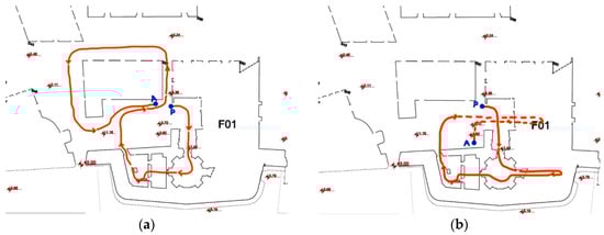
Figure 2.
The test footpaths: (a) path 1, closed; (b) path 2, open, with an elevation difference from the start point (P) to the end point (A).
The duration of the walk along the test paths was, for all the systems, about ten minutes.
2.4. “Ground Truth” and Dataset Alignment
As stated in Section 2.1, it is very difficult to analytically predict the accuracy of the final position starting from the IMMS components of instrumental error; therefore, the data assessment presented in this study is produced by comparing each resultant mapping with the “ground truth”.
For this, a sub-set of the available point model, previously acquired by Z+F 5010C TLS [28], was assumed. The scan alignment was performed thanks to 155 control points (black and white targets): their positions were defined by topographic measures based on a control network of 40 vertices in the inner part of the fortress. The topographic network and the control points were measured by the geodetic branch of the Italian Military Geographic Institute (IGMI). IGMI estimates network accuracy of less than one centimetre, and target accuracy of about one centimetre. The scan alignment, initially based on such targets, was then optimized by an ICP algorithm (implemented in Cyclone software, by Leica Geosystems), providing a mean absolute error of less than one centimetre. Considering the available data metrics, and the expected accuracy of the IMMS under testing, it is possible to assume the former as a reliable reference.
A cloud of about 1250 million points was then available as the ground truth: first of all, it was cleaned up by removing cars, passers-by, etc. and, later decimated to clouds with 1-cm resolution (as specified further on), in order to make the resolution not only more regular but more comparable to that of the datasets under examination. At the end, two reference datasets were created, with the data acquired by following the two planned paths: a first dataset of about 67 m × 78 m with 69,785,238 points for path 1, and a second of about 43 m × 48 m with 33,483,564 points for path 2. In both cases, the maximum elevation difference in the datasets is about 25 m.
The three examined IMMSs provided data in different reference systems: the Stencil and Zeb-Revo are defined arbitrarily, while the Pegasus produces WGS84 coordinates according to GNSS measurements which are transformed into a local vertical datum. Therefore, all of them needed to be transformed to use the same reference system as the ground truth (a local datum in a Gauss conformal projection that was specifically designed to avoid cartographic deformations). For this purpose, the widely used and open source CloudCompare software [29] was employed. First of all, a rough alignment was obtained from the three IMMS clouds by rotating and translating them, and suitably defining four corresponding points in all of the datasets. These points were chosen as far away from each other as possible in the whole test area: the same natural features were picked up in all the datasets. As a result, the four clouds were roughly pre-aligned, while the final refinement was obtained using the ICP algorithm, again with CloudCompare software. Hence, the ICP algorithm was used in a traditional manner, and not for “SLAM purposes” as in Section 2.1.
As is known, the ICP process randomly considers a sub-sample of the point clouds at each iteration; we noticed that the default value proposed for the “random sampling limit” parameter affected the results. Due to the very large point models considered, we increased its value to 2 million points to strike a balance between the computation speed and reliability of the results. Table 1 summarizes the signed distances (RMS Root Mean Square) after ICP alignments of the IMMS clouds.

Table 1.
RMS of signed distances after iterative closest point (ICP) alignments of the indoor mobile mapping system (IMMS) clouds.
2.5. Quantitative Criteria for the Evaluation
Due to the complexity of the process of generating the final point clouds, it is difficult not only to predict their accuracy, but also to define the general and objective procedures to assess the IMMS considered. In any case, some operative rules have to be set beforehand for the data acquisition in order to acquire as many comparable point clouds as possible: for instance, survey resolution is related to the walking speed, the way how the handheld systems are held affects the completeness of the model, the path should be even to avoid sudden turns, large differences in the ground influence the obtainable results, and so on. Furthermore, raw data are stored in proprietary format and are not homogeneous, therefore we were not able to consider them. Data elaboration is generally performed (the Kaarta system is an exception) during post-processing, with dedicated software. Different algorithms, none of them open source or supported by accessible scientific documentation, are implemented, and a great number of parameters have to be set up.
As said earlier, we considered the data provided to us by the producers to be the best acquired and post-processed result. The number of surveyed points varies depending on the IMMS and path, from a minimum of 7 million acquired with the Zeb-Revo in path 1 to a maximum of nearly 100 million measured with the Leica Pegasus in path 2; all of the values are later reported.
Various analyses can be conducted on these IMMS clouds, once aligned in the same reference system as reported in Section 2.4, of course reserving a fundamental role for the ground truth cloud. More in general, the evaluation of the correctness and accuracy of a point cloud can be carried out by following at least these three approaches: cloud to cloud [30], point to point [31], and cloud to feature [32,33] comparisons.
2.5.1. Cloud to Cloud Comparisons
Comparisons between high resolution datasets are a key issue in change detection studies [34]. Examples of applications are for the assessment of natural surfaces altered by erosion, and for measuring the extracted volume of material in quarry management. Techniques based on the comparison of digital elevation models DEMs in a geographic information system GIS environment (DEM of differences, DoD) can be substituted by cloud to cloud (C2C) or cloud to a triangulated mesh (C2M) comparisons any time a comparison between complex-shaped and not-quite-plane scenes has to be taken into account. In 2013, Lague et al. proposed the Multiscale Model to Model Cloud Comparison algorithm (M3C2) [35], which is implemented in CloudCompare as a plugin. It starts by estimating the normal surface and orientation in 3D at a scale consistent with the local surface roughness. Then, it measures the mean surface change along the normal direction and explicitly calculates a local confidence interval. M3C2 directly compares two point clouds by using a sample of core points (a subset of the original one, to speed up the computations).
With respect to C2C and C2M methods, M3C2 provides an easier and quicker workflow because it does not require a meshing process and it reduces the uncertainty related to point cloud roughness by local averaging. Moreover, M3C2 provides signed (and robust) distances between two point clouds [36]. For these reasons, we adopted the M3C2 algorithm to analyse the IMMS datasets in order to obtain statistical parameters about the signed distances, as well as an interactive 3D view of the dataset comparison. This supports the data quality assessment, which is of course related to the test field shape and characteristics.
An aspect complicating the comparison is that, in general, datasets acquired with any IMMS do not completely overlap with the reference, since many high surfaces are not scanned. Therefore, it is important to set a threshold value beyond which the distance is not computed. In the M3C2 CloudCompare procedure, a “maximum allowable distance” can be specified to eliminate unrealistic results when the compared clouds have different extensions or when datasets are spatially discontinuous: in this study, a distance of one metre was assumed.
All of the data comparisons are stored as scalar fields and are presented hereinafter by mapping the values onto the IMMS tested. The same colour scale is adopted for all the figures in the Results section. The colour scales are presented (in metres) on the right of the figures; the range scale of the signed distance values varies from −1 m to +1 m but, to improve their readability, the rainbow colour scale only considers a −8 cm to +8 cm range.
2.5.2. Point to Point Comparisons
Compared points should be considered as “derived points”, since they are extracted from a high-resolution dataset as “representing” corners or other features [22].
Some 14.5-cm-diameter spheres were placed on the scene and we initially planned to use their centre coordinate, extracted using a best fitting process, to compare the relative distances with respect to the topographic measurements. Unfortunately, the low resolution and the high noise level in all of the considered datasets prevented the extraction of significant data from these spheres. For this reason, they were used later as comparative features for qualitative analysis only.
A more extensive point to point comparison was done by extracting corresponding 0.5-cm-wide slices from the clouds along defined planes: Figure 3 shows in red one horizontal slice obtained for the dataset of the closed path 1 and the position of two vertical section planes allowing the extraction of vertical slices.

A close visual examination of the comparison between IMMS versus ground truth slices not only shows local misalignments (Figure 4), but also the remarkable noise in the data and sometimes the presence of “double surfaces” (Figure 5). Slice comparisons are considered for supporting local qualitative evaluations and are described later.
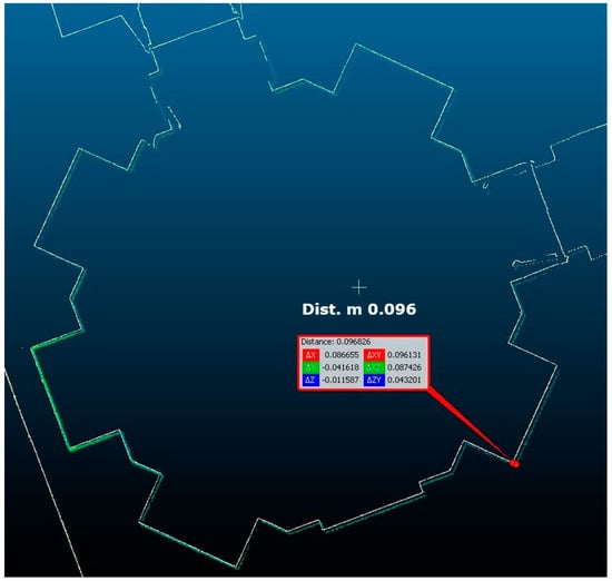
Figure 4.
Path 1—Comparing datasets: Leica Pegasus in colour versus reference data in white. The horizontal section in the octagonal room (4.3 m above floor level) shows local misalignments.
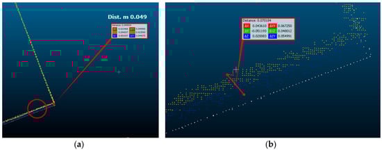
Figure 5.
Path 1—Comparing datasets: Leica Pegasus (a). The enlargement (b) highlights the noise and the misalignment between the data acquired, on the same facade, at different times (yellow and blue).
2.5.3. Cloud to Features Comparison
When objects or features with a known geometry are available on the scene, the surveyed model can be assessed by comparing it with the models known a priori. Reference surfaces can be spheres, cylinders, flat planes, or more complex objects.
In our case, it was not possible to build reference objects of a suitable size for the test underway. Instead, it was preferred to assume some surfaces on objects facing the scene and consider them as “features”, as later described in Section 3.4.1. For this purpose, cloud to mesh distances were computed in CloudCompare. For each point of the compared cloud, the C2M tool searches for the nearest triangle in the reference mesh and provides the signed distance, given that the normal is known for each triangle of the mesh. The results are displayed by mapping distances on a dataset in a suitable colour scale.
2.6. Qualitative Criteria for the Evaluation
In addition to the quantitative evaluation described above, some qualitative considerations can be helpful in providing a more exhaustive overview of the performances of the tested systems.
2.6.1. Quantity of Data and Data Completeness
Even though the paths covered with all the systems were the same and two of them (Stencil and Pegasus) incorporated the same laser sensor (Velodine VLP-16), the final models consist of a very different number of points. The extension of the model around the paths also varies. The asset of the linear laser, with more or less lining, fixed or movable by the user during the acquisition, affects the availability of a complete model, in particular with regard to the higher surfaces, like in the case of closer facades and vaults.
2.6.2. Feature Recognizability
With the aim to assess the quality of the recorded data under practical measurement conditions, particularly with regard to documenting the Cultural Heritage, the ability to resolve small object details should be considered. The complete point model is the final output of an IMMS survey, but, at the same time, it is the starting point for further elaboration relating to different application fields.
In general, the possibility of recognizing features on the 3D model is related to accuracy, resolution, and noise level. In IMMS, it is difficult to evaluate all of these aspects separately. For instance, when focusing only on the laser, the accuracy and resolution are limited by the measured distance. The laser beam has a spot diameter, which also increases with the distance, and angular inaccuracy affects the data depending on the slant of the measured surface. This does not affect the measurement of large and flat objects, but the recognizability of small objects can be compromised. Since it was not possible to set up a specific test site with expressly designed benchmark features, as done for TLS benchmarking by Böhler [37], we chose to evaluate the ability to record real-world objects and details: we compared the data acquired around flat black and white targets (21 cm × 30 cm), white spheres (14.5 cm diameter) hung on the walls, and some architectural details such as doors and windows.
2.6.3. Wrong Double Surfaces
Repeatability seems to be a weak point of IMMS. Even though the accuracy is within the expected range, in some cases when an object is acquired twice, in different parts of the same path the final model presents some double or “fake” surfaces.
3. Results
3.1. Kaarta Stencil
3.1.1. Data Acquisition
Data are acquired and aligned in quasi real time (Figure 6), without any post-processing thanks to the LOAM approach mentioned in Section 2.2.1. Consequently, in principle, it is possible to interrupt the acquisition at any time, and no difference is expected whether following an open path or a closed loop. In truth, during our examination, in path 2, the system unexpectedly stopped recording data (see green dot in Figure 6b) and unfortunately it was not possible to recover them.

Figure 6.
Kaarta Stencil datasets: (a) path 1; (b) path 2.
3.1.2. Dataset Evaluation
The values of standard deviation of the signed distances are respectively 7 cm for path 1 and 5 cm for path 2: these values, as well as the corresponding ones for the other two tested systems, summarize the discrepancies with respect to the reference dataset (see Table 2). This gives us a first overall indication of the accuracy obtainable by an IMMS surveying in similar conditions, although further statistical inference analysis should be carried out, for example based on robust non-parametric tests as suggested in [11]. Anyway, a relative comparison between the RMS values of the 5different paths and/or IMSSs gives an idea of how each system works on average in the experimented conditions.
Table 2.
The RMS of signed distances of IMMS datasets with respect to the ground truth.
Figure 7a and the corresponding figures for the other two systems display main discrepancies in three areas with trees, acquired in path 1: it is quite impossible to compute and evaluate the distances, and since the numerical values fluctuate between −1 and 1 m they are meaningless for the test. Instead, among those surfaces with significant differences, the IMMS points with most errors are the farthest from the acquisition trajectory, such as points on the eaves, which are approximately 15 m high.
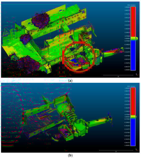
Figure 7.
Signed distances of the Kaarta Stencil dataset compared to the ground truth: (a) path 1; (b) path 2.
The data acquired with the Stencil are the least complete in our test, in particular for the vaults in the indoor areas. This is due to the fact that the system was held almost vertically, thus collecting data with a horizontal field of view of only 30°. Therefore, in small and indoor spaces the upper part of the surfaces was not scanned.
The system experienced some troubles when walking through narrow passageways, as was evident after the sequence of two doors (see details in the red circle in Figure 7a and recall the trajectory direction of Figure 2). A threshold distance was set to avoid scanning the operator walking with the system: probably the value of 2 m during our test was too high and it prevented data on closer surfaces from being recorded, which might have been useful. Figure 8 shows details of the horizontal section in those rooms and it highlights the increased misalignment after these passageways: up to 14.6 cm in the room with a large (170 cm × 110 cm) brick pillar in the centre. The blue points (highlighted in the circle) show the relevant data in the elevation of the floor.
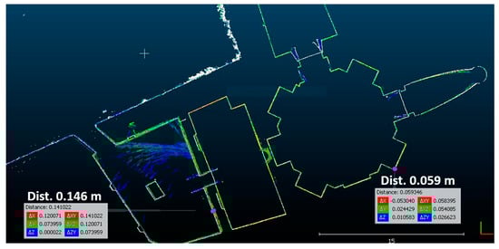
Figure 8.
Kaarta Stencil, path 1. Detail of the horizontal section (reference data in white, compared dataset in colour).
When looking at the vertical section crossing this room (Figure 9), the problem is even more evident: the rotation of the shape of the floor is wrong, with a level arm effect affecting the resulting elevation of the floors, and error values of as much as 79 cm downwards and 68 cm upwards on either side of the pillar. More in detail, incorrect negative elevations arose in the left part, where the operator walked with the IMMS, while they are positive in the right part, which was surveyed with rays not hidden by the pillar. Our interpretation of these gross errors is that the instantaneous rotation values of the scanning device are not well corrected by the “matching clouds” algorithm when the points are extremely close together, as occurred when entering this room by means of a small gate of only 135 cm × 140 cm in a 125-cm-wide wall, like a sort of “small tunnel”. This rotation error affected the successive acquisition of the left part of the room, causing a large counter-clockwise roll error, while this was wrongly overcompensated by the LOAM algorithm for the right part of the room. Better agreement with the reference data (with discrepancies of less than 10 cm), is instead visible in Figure 7, Figure 8 and Figure 9 in the “open” areas, for example, the octagonal room, whose “entry tunnel” gate measures 340 cm × 330 cm × 350 cm high.
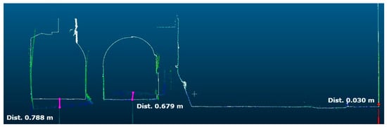
Figure 9.
Kaarta Stencil, path 1. Cross Section 1 (reference data in white, compared dataset in colour).
Regarding open path 2, Figure 7b shows similar discrepancies but, while Kaarta Stencil surveyed the same previous room precisely, following a similar trajectory, the system suddenly interrupted the acquisition, probably crashing during data processing owing to the presence of the points of the pillar. Hence, it was not possible to perform any evaluation in this room.
3.2. Leica Pegasus Backpack
3.2.1. Data Acquisition
As reported in Section 2.2.2, the Pegasus system incorporates a GNSS, even though it is supposed to work efficiently in indoor environments too. Compared to the other systems, it hence requires an initializing procedure, useful for both the GNSS and INS, consisting of walking for a few minutes in an outdoor space. At the end of the survey, an analogous process is required.
The scan data are acquired by the rear laser scanner, and hence it avoids recording data on the operator. A minimum measuring range of 40 cm makes this system suitable for very narrow places, even though it is bigger and heavier than the other two tested systems.
During our examinations, the surface textures were acquired by the cameras and the optional flash light was installed and turned on. The texture quality varies, with very interesting results in the small indoor spaces (the flash light range is about 6 m) but some overexposure is evident outdoors. In many applications, the image information can be very helpful to support the data interpretation and to provide engaging models for visualization purposes.
With Leica software supporting the Pegasus system, during post-processing it is possible to consider targets or natural points, if topographically measured, as constraints, and to use them for the linear adjustment of the scanned data, also by only considering a part of the whole trajectory. To make the acquired datasets (Figure 10) as comparable to the others as possible, we preferred not to use to this option.
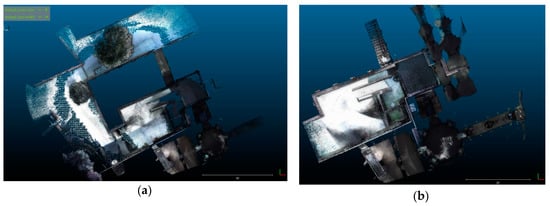
Figure 10.
Leica Pegasus Backpack datasets: (a) path 1; (b) path 2.
3.2.2. Dataset Evaluation
Other significant differences were detected in a particular area of the courtyard (circle D), where in reality the floor surface looks the same as the surroundings: this error is quite unexpected, and it could tentatively be explained as a local error in the procedure to close the path. Hence, after surveying this floor twice, two horizontal noised surfaces are obtained. It is important to remember that the same closed trajectory did not cause such discrepancies for the other two systems.
To confirm this supposition, if we are to observe open path 2 in Figure 11b, the same area does not present such errors: obviously no changes occurred between the two acquisitions, as the last one was carried out just a few minutes after the first one. It is interesting to see how the octagonal vault is surveyed more accurately now. Nevertheless, some other local errors can be noticed in the circled areas E and F. The vault ceiling (E) in the room before the octagonal room has a positioning error sharing negative (blue) and positive (red) values, similar to those of the octagonal vault for path 1, due to a roll effect. Errors in the courtyard (F) are more evident in the part acquired immediately outside, where again an error in TLS roll estimation causes errors in the positioning, and above all in the elevation of the far points.
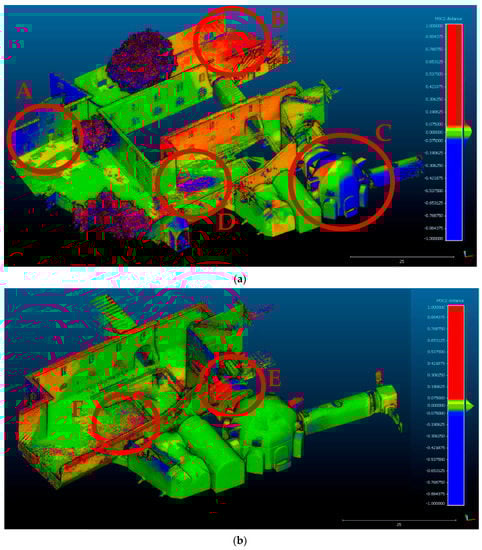
Figure 11.
Signed distances of the Leica Pegasus Backpack dataset compared to the ground truth: (a) path 1; (b) path 2.
Like in the Stencil dataset, the further and foreshortened points are less reliable and present both positive and negative distances of about 8 cm from the reference (Figure 12).
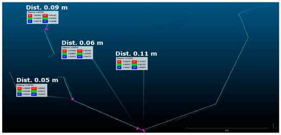
Figure 12.
Leica Pegasus Backpack, path 1. Horizontal section of the octagonal vault.
As a general consideration, the data acquired along open path 2 are closer to the reference with respect to those acquired along closed path 1: this seems rather surprising since the closing procedure should instead better compensate and distribute the errors in the TLS positioning and attitude.
Coming back to the situation of the room with a central pillar in Figure 9 with the Stencil data, in the slices of the cross section in Figure 13, the Pegasus cloud from path 2 presents a very correct and also complete description of the spaces, with point to point differences of less than 5 cm compared to the reference data. Since the covered trajectory is nearly always the same, we can assert that, in this particular geometrical situation, the SLAM algorithm works better than the LOAM algorithm.
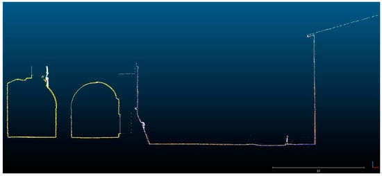
Figure 13.
Leica Pegasus, path 2. Cross Section 1 (reference data in white, compared dataset in colour).
3.3. GeoSlam Zeb-Revo
3.3.1. Data Acquisition
The Zeb-Revo has a field of view of 270° × 360°, which is achieved thanks to rotating the Hokuyo single-profile laser. Hence, this prevents data on the operator from being recorded. Nevertheless, on comparing Figure 14 with the corresponding Figure 6 (Stencil) and Figure 10 (Pegasus), the maximum range is shorter than the other systems.

Figure 14.
GeoSlam Zeb-Revo datasets: (a) path 1; (b) path 2.
Even if it is declared that the Zeb-Revo registers the normal surface, in the data we analysed, normal information was not present.
3.3.2. Dataset Evaluation
As a general consideration, in the common areas the Zeb-Revo and Pegasus are the most comparable systems, since both allow the ceilings of the internal test field to be surveyed, while the Stencil generally does not, as explained in Section 3.1.2. Although the Zeb-Revo resolution on higher surfaces is lower than with the Pegasus, the distances to the reference are usually smaller. In fact, the standard deviation of the distances is now respectively 4.0 cm for both path 1 and path 2, lower than that computed for the Pegasus data.
In Figure 15a, the points of path 1 are mostly green-coloured, and some of the red and blue ones relate to the tree canopy seen earlier. In Figure 15b, the colour of the points acquired in path 2 is “not green” (namely with an error of more than 8 cm) mainly in the passages between different rooms. This aspect requires a more attentive analysis. Nevertheless, the magnitude of error is less than ten centimetres. Moreover, considering a vertical cross section (Figure 16) similar to those in Figure 9 and Figure 13 but now along the orthogonal direction 2, there is no evidence of any remarkable misalignment or noised data in those areas. Some local point to point distance checks report very small values of 2–4 cm.
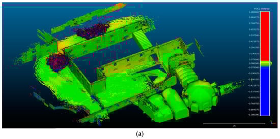
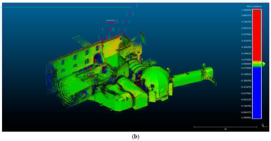
Figure 15.
Signed distances of the GeoSlam Zeb-Revo dataset compared to the ground truth: (a) path 1; (b) path 2.
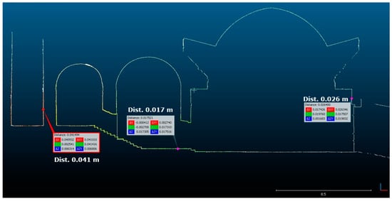
Figure 16.
GeoSlam Zeb-Revo, path 1. Cross Section 2 (reference data in white, compared dataset in colour).
To conclude Section 3.3, the results reported in Section 3.1.2, Section 3.2.2 and Section 3.3.2 give an idea of the various potentials and limits of the systems examined in our test field. The most important quantitative values are the obtained discrepancies, reported in Table 2 in the form of the root mean square of the signed distances. They show how on average for an IMMS survey there is a difference of less than 8 cm with respect to a TLS static survey, and this difference is reduced up to 4 cm for the Zeb-Revo cloud. For the same IMMS, the obtained signed distances for cloud from closed and open paths present similar mean values.
3.4. Assessment of the Models’ Level of Detail and Feature Recognizability
Further to the quantitative results above reported, looking at the models obtained, they also differ in other aspects that are not easy to quantify and that can be only described qualitatively. In general terms, they are strictly related to the noise level and to the model resolution, both influencing the “level of detail” (LoD) of the obtained models. While noise level mainly depends on the TLS system (as well as on the algorithms applied in post-processing), resolution is strongly dependent on acquisition speed. Therefore, an improved working mode in order to enhance the obtainable LoD can simply be to slow the walking speed in the proximity of objects of special interest.
As already reported in Section 2.6.2, some objects such as:
- planar black and white targets,
- spheres, and
- architectural details can be used to evaluate and compare the recognizability of features in the three clouds.
3.4.1. Target Recognition
Planar and three-dimensional targets can be useful for the Stencil and Zeb-Revo dataset geo-referencing even though, at present, only the Pegasus post-processing workflow can consider ground control points.
A simplified qualitative comparison of the target recognition in our test can be done by observing Figure 17, which shows a 20 cm × 20 cm black and white target attached to a wall. In the Stencil and Zeb-Revo datasets (for both paths), it is totally impossible to recognize this planar target, while it can just about be identified in the Pegasus dataset only (Figure 17, second row). The clouds in Figure 17 also highlight the big differences in dataset resolution and clearly show the direction of the acquired profiles. It is important to stress that, for all of the datasets, the resolution varies greatly on the surfaces, being higher along the scanned profiles and lower between one profile and the next.
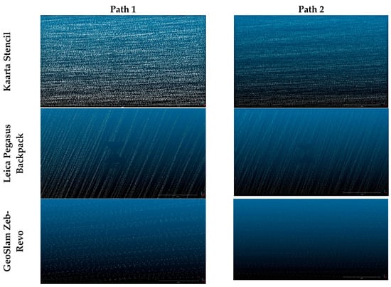
Figure 17.
Various datasets in correspondence to a black and white target on a wall: in addition to the difficulty in recognizing the target, it is visible how the resolution along the vertical and horizontal directions changes dramatically.
3.4.2. Sphere Recognition
Six calibrated spheres (designed for Faro TLS data alignment) were placed along the paths. They were attached to the wall with a specific support holding them about 10 cm away from the wall surface. The spheres were white and had a diameter of 14.5 cm. As can be seen in Figure 18, unfortunately they are still too small to be clearly extracted. Namely, the cloud LoD is not sufficient to recognize them and to precisely compute the centre.
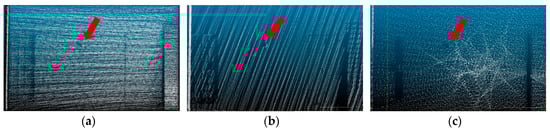
Figure 18.
Three datasets with a 14.5 cm-diameter sphere, pinpointed by the arrow, attached to a wall: (a) Kaarta Stencil; (b) Leica Pegasus Backpack; (c) GeoSlam Zeb-Revo.
Of course, the spherical and other solid targets are placed in the area to support the geo-referencing process. This was our intention so that the natural points in the alignment procedure described in Section 2.4 did not have to be chosen manually. The dimension of these targets must then be carefully considered and, in a situation similar to our test field, the spheres should have a diameter of more than 20 cm.
3.4.3. Recognition of Architectural Details
In order to assess the real usability of IMMS data in an urban/architectural environment, some comparisons were made with respect to the possibility of not only recognizing the main built volumes, but also some typical architectural details such as doors, windows, lamps, and so on.
First of all, in the test field, we considered the corner defined by two facades shown in Figure 19. Here, the recognizability of details from the static reference cloud (b) can be easily appreciated.
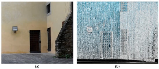
Figure 19.
Corner of the chosen building for assessing the recognizability of architectural details; (a) photo; (b) reference dataset statically acquired by terrestrial laser scanning (TLS) and down-sampled with 1-cm average resolution.
On observing Figure 20, the same linear scanning direction in Figure 17 and Figure 18 is clearly visible, here denoting a denser resolution: in the Stencil and Pegasus datasets, the different TLS tilt during acquisition is evident. The Stencil’s linear laser rotates around a pseudo-vertical axis (therefore the profile tracks are almost horizontal), while the Pegasus’s laser rotates around a pseudo-horizontal axis (so the profile tracks are almost vertical). The Zeb-Revo resolution is instead more homogeneous thanks to the rotating acquisition system. On the other hand, the Zeb-Revo dataset resolution is lower, and the same considered features are barely recognizable.
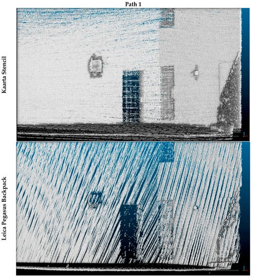

Figure 20.
Area chosen for assessing the recognizability of architectural details in the clouds.
In sum, in this part of the test field, only the Stencil cloud has an LoD enabling the reconstruction of “small objects”, namely architectural details.
All of the datasets in Figure 20 are visualized in the CloudCompare environment, without any shading or visualization improvements. As is well known, rendering techniques can significantly modify the effectiveness of data visualization and exploration, so for each dataset we tried to set up the best way to render it: obviously, this is an arbitrary and subjective choice, but it aims to qualitatively use the acquired clouds in the best way possible.
For this purpose, we considered the two walls of the aforementioned octagonal room, shown in Figure 21. To be compared with the other datasets acquired without texture, the Pegasus dataset is also visualized with intensity values in Figure 22.
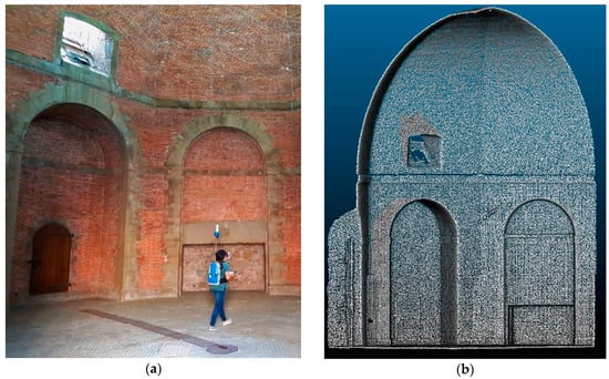
Figure 21.
Octagonal room—data visualization assessment; (a) photo; (b) TLS reference dataset.
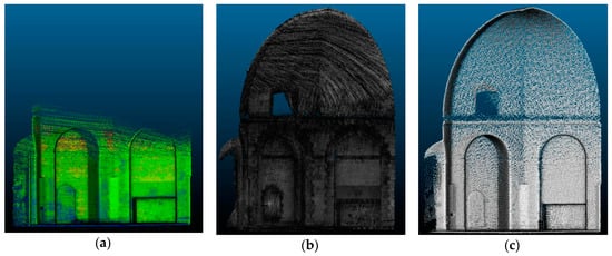
Figure 22.
Octagonal room—data visualization assessment; (a) Stencil; (b) Pegasus; (c) Zeb-Revo.
On comparing the representations in Figure 22, despite missing the upper part, the intensity readability of the Stencil cloud is good, with a similar colour scale to the scales of grey Pegasus data; the grey scale intensity of the Zeb-Revo instead has a very poor interval and is not very readable.
3.4.4. Double-Surface Evaluation
Finally, we wanted to investigate why in some parts of the maps presented in Section 3.1.2, Section 3.2.2 and Section 3.3.2 the data referring to the same surface are mapped with different colours on the opposite sides, and even present opposite signs. Therefore, we considered a part of a building defined by three plane orthogonal facades and we compared the test datasets with the mesh surface from the TLS data again as a reference.
The comparison was done with the C2M tool in CloudCompare on the datasets acquired in path 1 and the results are shown in Figure 23. The Stencil and Zeb-Revo essentially confirm the general results displayed in Figure 7a and Figure 15a. Here they are more detailed with a histogram of the signed distances: in both cases, the data are distributed around a slightly different value from zero, but they are essentially symmetrical. Here the Pegasus dataset instead produced a trimodal distribution of differences, one prevalently coloured in blue (negative values), one in green (values around zero), and one in yellow-orange (positive values). These colours hence represent the prevalent distance from the reference, whose modes are respectively −8, −1, and +7 cm: the first two correspond to two “surfaces”, parallel to a real wall facade, as visible in the slice in Figure 24. Note how these two clouds are not clearly recognizable in the frontal representation of Figure 23, where a green coloration is instead dominant. Conversely, the point error on the other, orthogonal façade is represented in a yellow-orange colour.
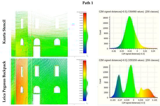
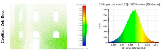
Figure 23.
Comparison between the datasets under examination and a meshed reference. On the right are the histograms of the signed distances. C2M: cloud to mesh.
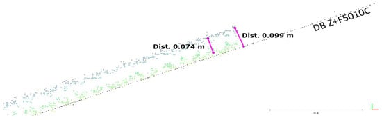
Figure 24.
Leica Pegasus Backpack, detail of a horizontal slice of data shown in Figure 23 (reference data in black, compared data in colour).
3.5. Qualitative Evaluation Table
A summary of the assessment of the qualitative criteria previously described is finally presented in Table 3, where the final scores are given by the average evaluation of five operators who are experts in architectural representation. It is clear that this is a subjective assessment and it is strictly related to the particular test field in question. Nevertheless, the reported judgements sum up what was found throughout this work.
Table 3.
Subjective evaluation of qualitative criteria considered in the test.
Other non-negligible parameters, such as the weight or price of the system, are not considered here.
4. Conclusions
In order to examine the performance and limitations of different indoor mobile mapping systems (IMMSs), knowledge of the basic principles of measurement of this advanced surveying methodology (Introduction, Section 1) has been reviewed. IMMSs represent one of the most promising areas of geomatics for their outstanding capability to acquire the coordinates of millions of points in a very short time, by simply walking in the area of interest.
Nevertheless, the complex analytical model is implemented by different algorithms (Material and Methods, Section 2.1) and it can be considered as a two-step process. Firstly, there is multi-sensor mapping, where instrumental hardware efficiency plays a key role, followed by a refinement, generally called SLAM. This is not really simultaneous process, and thus it is impossible to predict the final correctness and accuracy obtainable from a given IMMS. Besides, it is difficult to compare different systems, also considering that hardware/software configurations can dramatically change from one to another and, above all, that the final results are strongly influenced by the adeptness of the software. A comparative procedure is proposed here with the paper considering the point clouds obtained by the Kaarta Stencil, Leica Pegasus Backpack, and GeoSlam Zeb-Revo systems (Material and Methods, Section 2.2). The test field (Material and Methods, Section 2.3) was chosen to as far as possible reproduce real, variable conditions; therefore, a closed and an open footpath were defined, with both considering internal and external environments. The test area was previously measured by means of static scans with a Z+F TLS, which were assumed to represent the “ground truth” (Material and Methods, Section 2.4). The three IMMS clouds were then aligned in the same reference frame as the ground truth. After that, quantitative criteria were fixed for the evaluation (Material and Methods, Section 2.5): cloud to cloud, point to point, and cloud to feature distances were assessed. Finally, qualitative criteria (Material and Methods, Section 2.6) were defined for additional evaluations.
A large part of the paper is devoted to describing data acquisition (sometimes with operating problems) and to discussing the test results for each system (Results, Section 3.1, Section 3.2 and Section 3.3), with quantitative evaluations (Results, Section 3.4) of the differences between the datasets under examination and the reference cloud.
To summarize the results provided by the tests, the Stencil and Pegasus Backpack data present distances of less than 8 cm with respect to the reference, while the Zeb-Revo data present smaller discrepancies. For all the systems, these mean distances are quite similar for datasets acquired by following the closed or the open path.
The qualitative evaluation (Results, Section 3.4) concerns the completeness of the data, modelling of the artefacts, and level of detail of the three clouds enabling the targets, spheres and architectural details to be recognized (or not). It is only possible to “glimpse” the targets with the Pegasus Backpack, while none detect the 14.5-cm-diameter spheres. Regarding the description of the architectural features, the scanning direction assumes crucial importance: the Stencil’s very dense horizontal profiles allow the best interpretation, followed by the Pegasus’s dense vertical profiles and then by the Zeb-Revo’s “low”-density mixed profiles. To best recognize the architectural details through a manual process, the visualization of the data becomes crucial and, for this reason, this aspect was analysed too. Finally, the “double surfaces” produced by some of the systems on perfectly vertical and smooth walls were investigated: the Pegasus’s histogram of distances from the reference data shows the erroneous presence of twofold surfaces.
The results obtained in both the quantitative and qualitative assessments of our examination (Results, Section 3.5) cannot be generalized, in particular the negative ones. Nevertheless, some “tentative conclusions” can be outlined regarding the positive characteristics of the three tested systems, while remembering that there is a small difference in instrumental configuration and commercial costs between the Stencil and the Zeb-Revo and that these differences are a lot greater for the Pegasus. The Stencil is the only system we tested that is able to provide data immediately after the acquisition without any post-processing, and that allows the architectural features to be recognized better. The Zeb-Revo output clouds present smaller differences with respect to the reference data and the cross sections agree with the static TLS survey better too. The Pegasus provides the most complete model, with the intensity of the data enabling the identification of artificial features, and it is the only one allowing absolute geo-referencing thanks to the GNSS receiver.
To conclude, throughout the presented comparative examination, the IMMS performances and limits were analysed and investigated by testing commercial systems in a real scenario. Since on the market IMMSs are proposed for non-specialists in geomatics, we can imagine some common questions from a generic user interested in evaluating their effectiveness. A first Frequently Asked Question (FAQ) should be: “How precise is a particular IMMS?” A quantitative answer is not possible, because the accuracy, for the same system, still depends on the distance between the system and the object and the object may be in a very large open space. A second FAQ could be: “Which of these IMMSs is the most precise?” Also in this case, there is no single answer, since a lot of other qualitative aspects in the final results need to be considered.
As a general deduction, weighing up the pros and cons, the final judgement on the “young” IMMS methodology is extremely encouraging. In the near (imminent?) future, technological and theoretical research in progress will further hardware improvements and software implementations to further enhance this already efficient, albeit not perfect, geomatics system.
Acknowledgments
The authors wish to thank the following companies for providing the tested IMMS products: Me.s.a. s.r.l. as the supplier of the GeoSlam Zeb-Revo; MicroGeo s.r.l. for the Kaarta Stencil; and Leica Geosystems for the Pegasus Backpack. Special thanks go to the architects Lidia Fiorini and Alessandro Conti for the data processing. For providing access to the location and their helpfulness we thank the Municipality of Florence and engineer Federico Fabiani of Firenze Fiera S.p.A. Our gratitude also goes to the Italian Military Geographic Institute (IGMI) for the topographic support and to Brig. Gen. Enzo Santoro, Chief of the Geospatial Information Department, for coordinating the activities. The work has been funded as part of the Italian Research Project of National Interest “GAMHer—Geomatics Data Acquisition and Management for Landscape and Built Heritage in a European Perspective” (PRIN2015 n.2015HJLS7E) and the publication costs were covered by the University of Florence Department of Civil and Environmental Engineering (DICEA).
Conflicts of Interest
The authors declare no conflict of interest.
References
- Barsanti, S.G.; Remondino, F.; Visintini, D. Photogrammetry and laser scanning for archaeological site 3D modeling—Some critical issues. CEUR Workshop Proc. 2012, 948, B1–B10. [Google Scholar]
- Keller, F.; Sternberg, H. Multi-sensor platform for indoor mobile mapping: System calibration and using a total station for indoor applications. Remote Sens. 2013, 5, 5805–5824. [Google Scholar] [CrossRef]
- Corso, N.; Zakhor, A. Indoor localization algorithms for an ambulatory Human operated 3D mobile mapping system. Remote Sens. 2013, 5, 6611–6646. [Google Scholar] [CrossRef]
- Zlot, R.; Bosse, M.; Greenop, K.; Jarzab, Z.; Juckes, E.; Roberts, J. Efficiently capturing large, complex cultural heritage sites with a handheld mobile 3D laser mapping system. J. Cult. Herit. 2014, 15, 670–678. [Google Scholar] [CrossRef]
- Lauterbach, H.A.; Borrmann, D.; Heß, R.; Eck, D.; Schilling, K.; Nüchter, A. Evaluation of a backpack-mounted 3D mobile scanning system. Remote Sens. 2015, 7, 13753–13781. [Google Scholar] [CrossRef]
- Nüchter, A.; Borrmann, D.; Koch, P.; Kühn, M.; May, S. A man-portable, IMU-free mobile mapping system. ISPRS Ann. Photogramm. Remote Sens. Spat. Inf. Sci. 2015, II-3/W5, 17–23. [Google Scholar] [CrossRef]
- Schmitz, L.; Schroth, G.; Reinshagen, F. Mapping Indoor Spaces with an Advanced Trolley Equipped with Laser Scanners, Cameras and Advanced Software. GIM International, 12 October 2015. [Google Scholar]
- American Society for Photogrammetry and Remote Sensing. 1995 Mobile Mapping Symposium. In Proceedings of the First International Workshop on “Mobile Mapping Technology”, Columbus, OH, USA, 24–26 May 1995; American Society of Photogrammetry & Remote Sensing: Bethesda, MD, USA, 1995. [Google Scholar]
- Woodman, O.J. An Introduction to Inertial Navigation; Technical Report 696; University of Cambridge Computer Laboratory: Cambridge, UK, 2007; 37p. [Google Scholar]
- Thomson, C.; Apostolopoulos, G.; Backes, D.; Boehm, J. Mobile laser scanning for indoor modelling. ISPRS Ann. Photogramm. Remote Sens. Spat. Inf. Sci. 2013, II-5/W2, 289–293. [Google Scholar] [CrossRef]
- Nocerino, E.; Menna, F.; Remondino, F.; Toschi, L.; Rodriguez-Gonzalvez, P. Investigation of indoor and outdoor performance of two portable mobile mapping systems. In Proceedings of the SPIE Vol. 10332 Videometrics, Range Imaging, and Applications XIV, Munich, Germany, 25–29 June 2017. [Google Scholar] [CrossRef]
- Lehtola, V.V.; Kaartinen, H.; Nüchter, A.; Kaijaluoto, R.; Kukko, A.; Litkey, P.; Honkavaara, E.; Rosnell, T.; Vaaja, M.T.; Virtanen, J.-P.; et al. Comparison of the Selected State-Of-The-Art 3D Indoor Scanning and Point Cloud Generation Methods. Remote Sens. 2017, 9, 796. [Google Scholar] [CrossRef]
- Masiero, A.; Fissore, F.; Guarnieri, A.; Piragnolo, M.; Vettore, A. Comparison of low cost photogrammetric survey with TLS and Leica Pegasus backpack 3D models. ISPRS Int. Arch. Photogramm. Remote Sens. Spat. Inf. Sci. 2017, XLII-2/W8, 147–153. [Google Scholar] [CrossRef]
- Schwarz, K.P.; El-Sheimy, N. Kinematic multi-sensor systems for close range digital imaging. ISPRS Int. Arch. Photogramm. Remote Sens. Spat. Inf. Sci. 1996, XXXI-B3/W3, 774–785. [Google Scholar]
- Baltsavias, E.P. Airborne laser scanning: Basic relations and formulas. ISPRS J. Photogramm. Remote Sens. 1999, 54, 199–214. [Google Scholar] [CrossRef]
- Crosilla, F.; Visintini, D. External orientation of a mobile sensor system for cartographic updating by dynamic vision of digital map points. Bollettino di Geodesia e Scienze Affini 1998, 1, 41–60. [Google Scholar]
- Nüchter, A.; Lingemann, K.; Hertzberg, J.; Surmann, H. 6D SLAM-3D Mapping Outdoor Environments. J. Field Robot. 2007, 24, 699–722. [Google Scholar] [CrossRef]
- Kaarta Stencil. Available online: http://www.kaarta.com/stencil/ (accessed on 15 November 2017).
- Zhang, J.; Singh, S. LOAM: Lidar odometry and mapping in real-time. In Proceedings of the 2014 Robotics: Science and Systems Conference (RSS), Berkeley, CA, USA, 13–15 July 2015. [Google Scholar]
- Kaarta Stencil Technical Sheet. Available online: https://static1.squarespace.com/static/57f7e2b215d5dbb87f65e7b2/t/58cc4aa646c3c4081398dc8a/1489783463807/Stencil+spec+sheet+3.17+web.pdf (accessed on 15 November 2017).
- Kaarta. Measurement Accuracy of Lidar-based SLAM Systems. Available online: http://www.microgeo.it/public/userfiles/LaserScanner/Stencil%20Accuracy%20Tech%20Report-001.pdf (accessed on 15 November 2017).
- Zhang, J.; Singh, S. Visual-lidar Odometry and Mapping: Low-drift, Robust, and Fast. In Proceedings of the 2015 IEEE International Conference on Robotics and Automation (ICRA), Seattle, WA, USA, 26–30 May 2015; pp. 2174–2181. [Google Scholar] [CrossRef]
- Leica Pegasus Backpack. Available online: https://leica-geosystems.com/products/mobile-sensor-platforms/capture-platforms/leica-pegasus-backpack (accessed on 15 November 2017).
- Leica Pegasus Backpack Technical Sheet. Available online: http://leica-geosystems.com/-/media/files/leicageosystems/products/datasheets/leica_pegasusbackpack_ds.ashx?la=en (accessed on 15 November 2017).
- GeoSlam Zeb-Revo. Available online: https://geoslam.com/hardware/zeb-revo/ (accessed on 15 November 2017).
- GeoSlam Zeb-Revo Technical Sheet. Available online: https://geoslam.com/wp-content/uploads/2017/08/GeoSLAM-ZEB-REVO-Solution-v7.pdf (accessed on 15 November 2017).
- Bosse, M.; Zlot, R.; Flick, P. Zebedee: Design of a Spring-Mounted 3-D Range Sensor with Application to Mobile Mapping. IEEE Trans. Robot. 2012, 28, 1104–1119. [Google Scholar] [CrossRef]
- Tucci, G.; Bonora, V.; Conti, A.; Fiorini, L. Digital workflow for the acquisition and elaboration of 3D data in a monumental complex: The Fortress of Saint John the Baptist in Florence. ISPRS Int. Arch. Photogramm. Remote Sens. Spat. Inf. Sci. 2017, XLII-2/W5, 679–686. [Google Scholar] [CrossRef]
- CloudCompare (Version 2.9), GPL Software. Available online: http://www.cloudcompare.org/ (accessed on 15 November 2017).
- Girardeau-Montaut, D.; Roux, M.; Marc, R.; Thibault, G. Change detection on points cloud data acquired with a ground laser scanner. In Proceedings of the ISPRS Workshop Laser Scanning 2005, ISPRS Archives, Enschede, The Netherlands, 12–14 September 2005; Volume 36, pp. 30–35. [Google Scholar]
- Tsakiri, M.; Anagnostopoulos, V. Change. Detection in Terrestrial Laser Scanner Data via Point Cloud Correspondence. Int. J. Eng. Innov. Res. 2015, 4, 2277–5668. [Google Scholar]
- Ridene, T.; Goulette, F.; Chendeba, S. Feature-Based Quality Evaluation of 3D Point Clouds—Study of the Performance of 3D Registration Algorithms. Int. Arch. Photogramm. Remote Sens. Spat. Inf. Sci. 2013, XL-2/W2, 59–64. [Google Scholar] [CrossRef]
- Jung, J.; Yoon, S.; Ju, S.; Heo, J. Development of kinematic 3D laser scanning system for indoor mapping and as-built BIM using constrained SLAM. Sensors 2015, 15, 26430–26456. [Google Scholar] [CrossRef] [PubMed]
- Rychkov, I.; Brasington, J.; Vericat, D. Computational and methodological aspects of terrestrial surface analysis based on point clouds. Comput. Geosci. 2012, 42, 64–70. [Google Scholar] [CrossRef]
- Lague, D.; Brodu, N.; Leroux, J. Accurate 3D comparison of complex topography with terrestrial laser scanner: Application to the Rangitikei canyon (N-Z). ISPRS J. Photogramm. Remote Sens. 2013, 82, 10–26. [Google Scholar] [CrossRef]
- CloudCompare Wiki. Available online: http://www.cloudcompare.org/doc/wiki/index.php?title=Main_Page (accessed on 15 November 2017).
- Boehler, W.; Bordas Vicent, M.; Marbs, A. Investigating laser scanner accuracy. Int. Arch. Photogramm. Remote Sens. Spat. Inf. Sci. 2003, 34 Pt 5, 696–701. [Google Scholar]
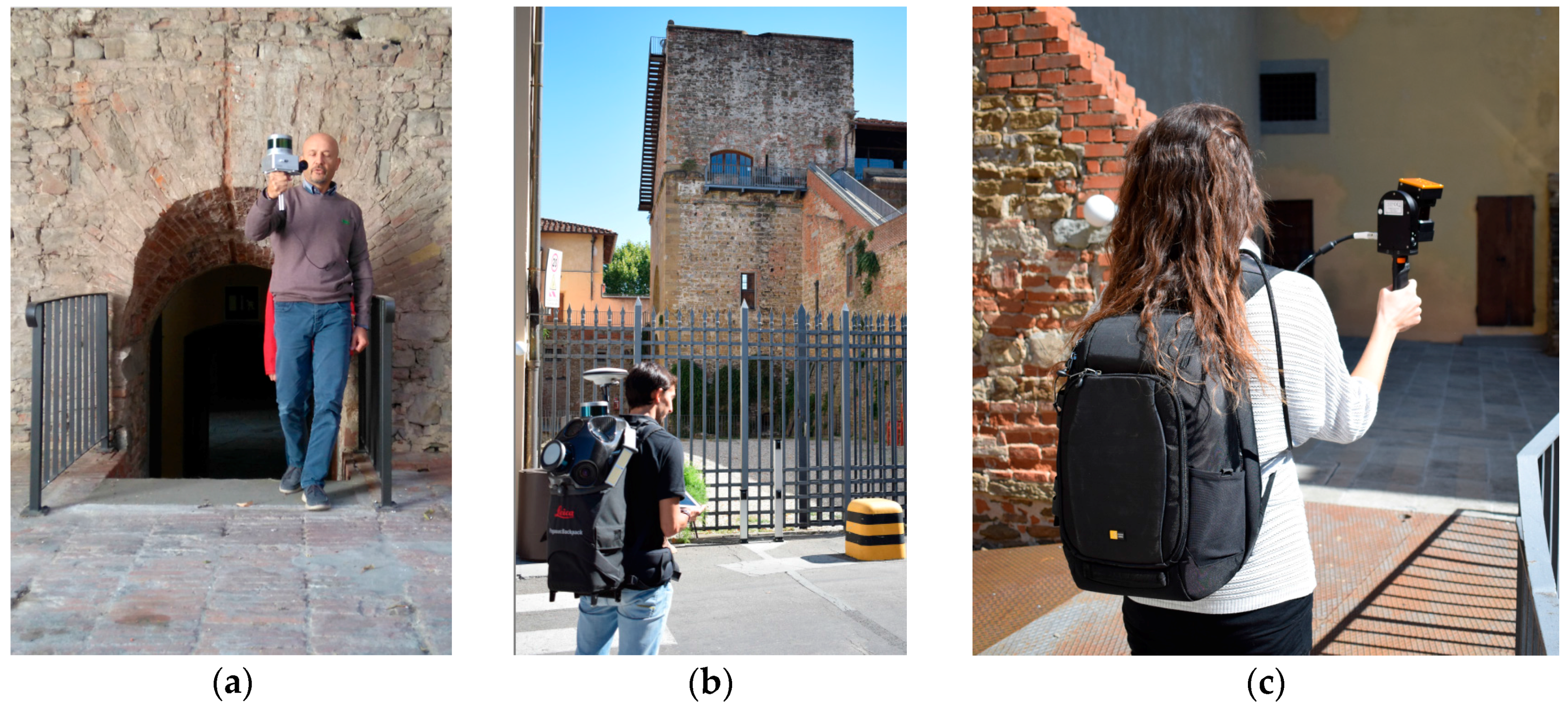
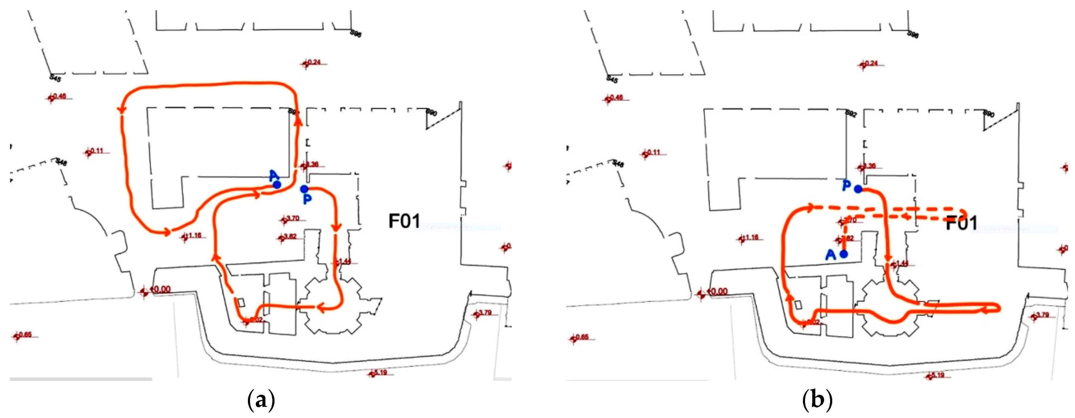
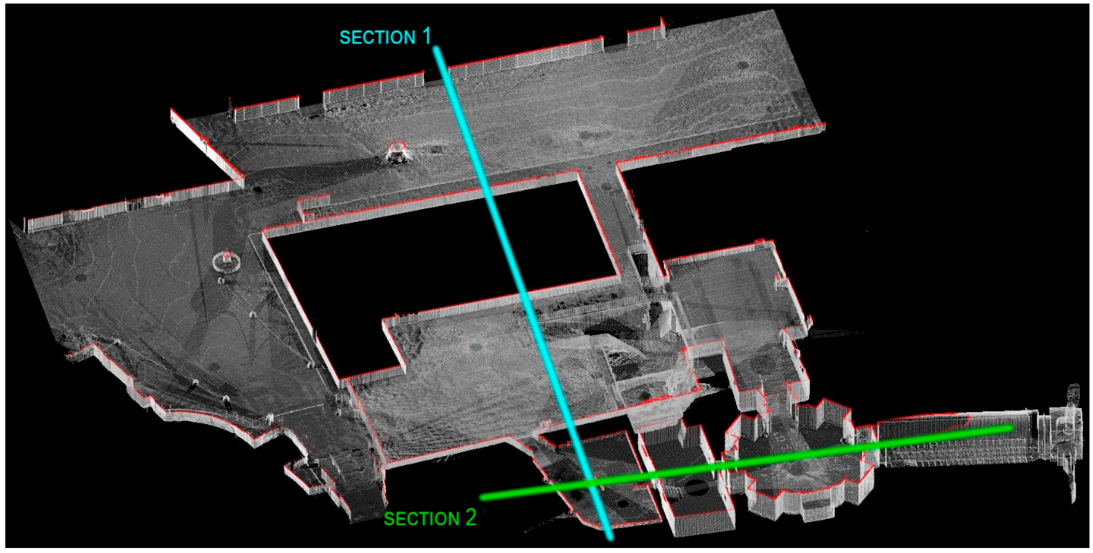
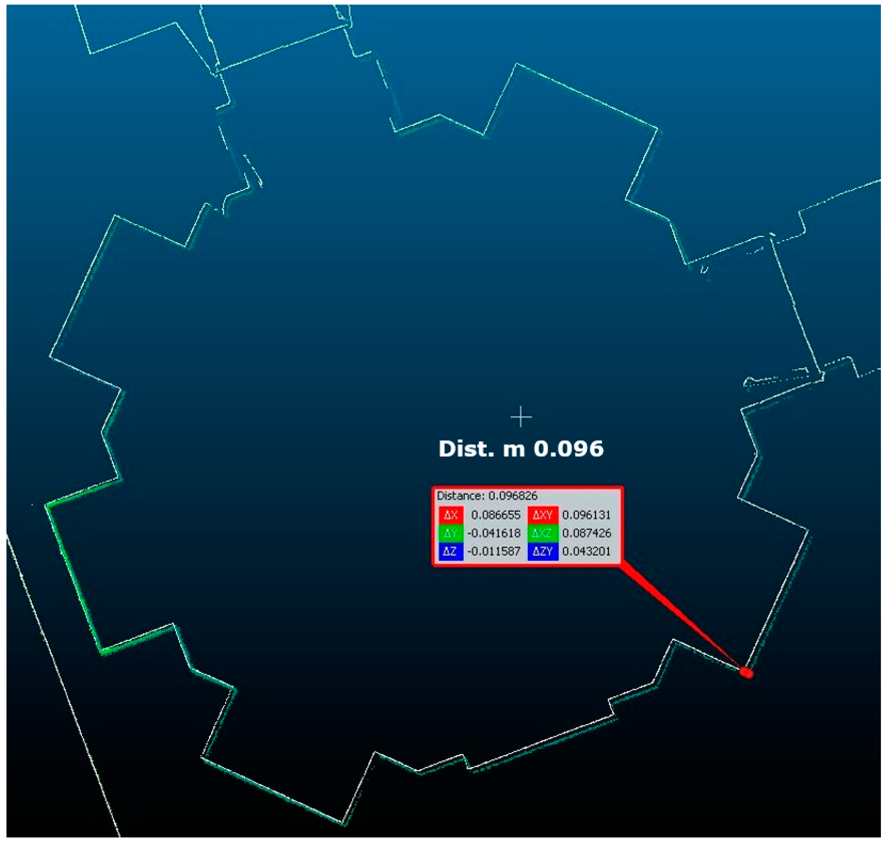
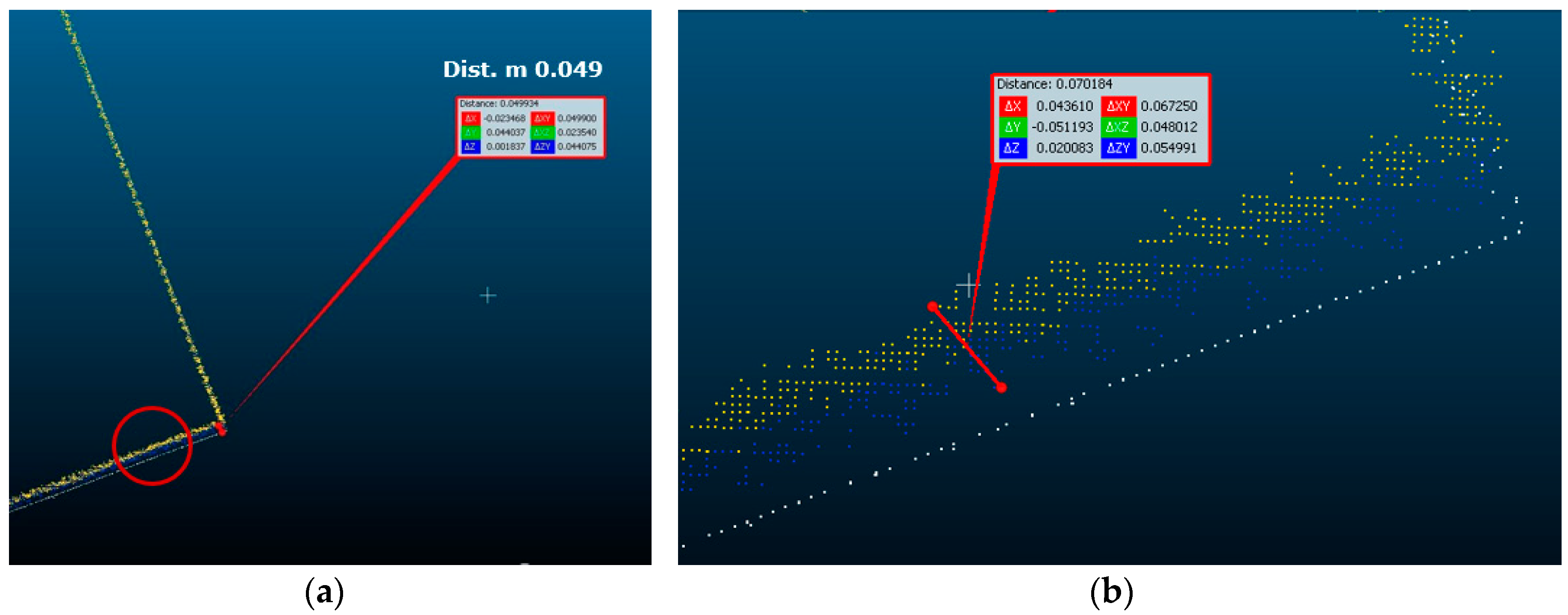
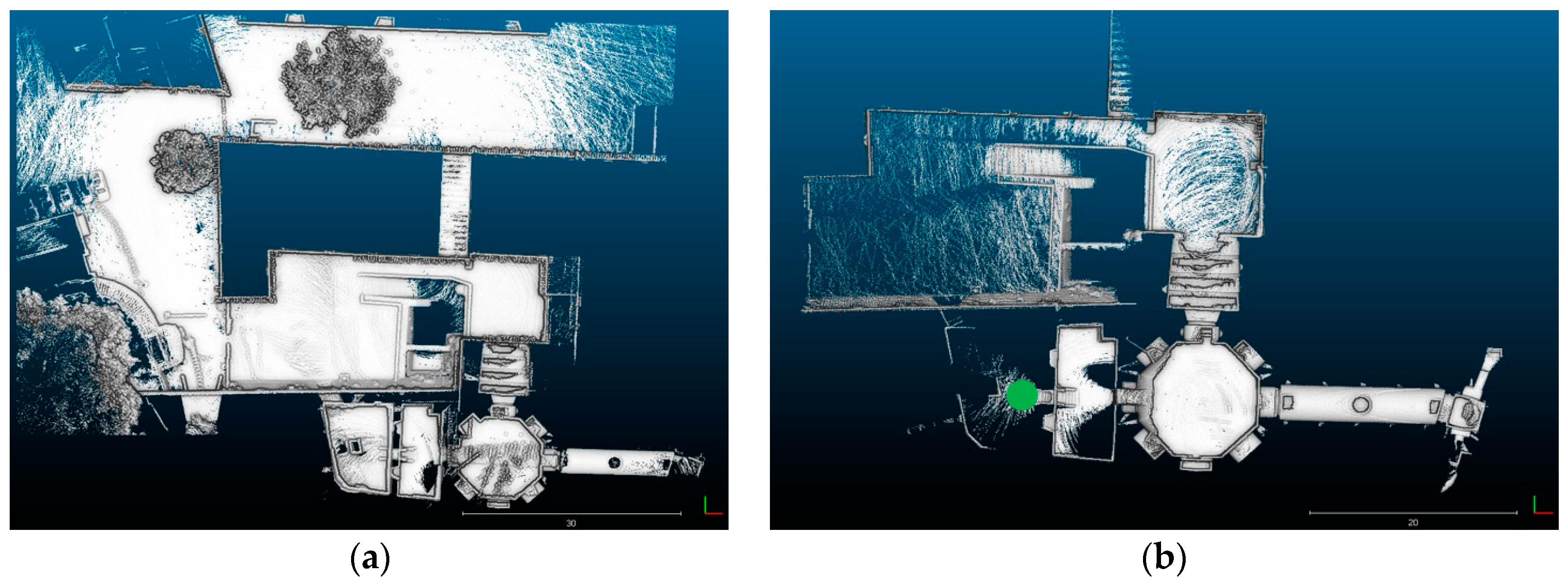

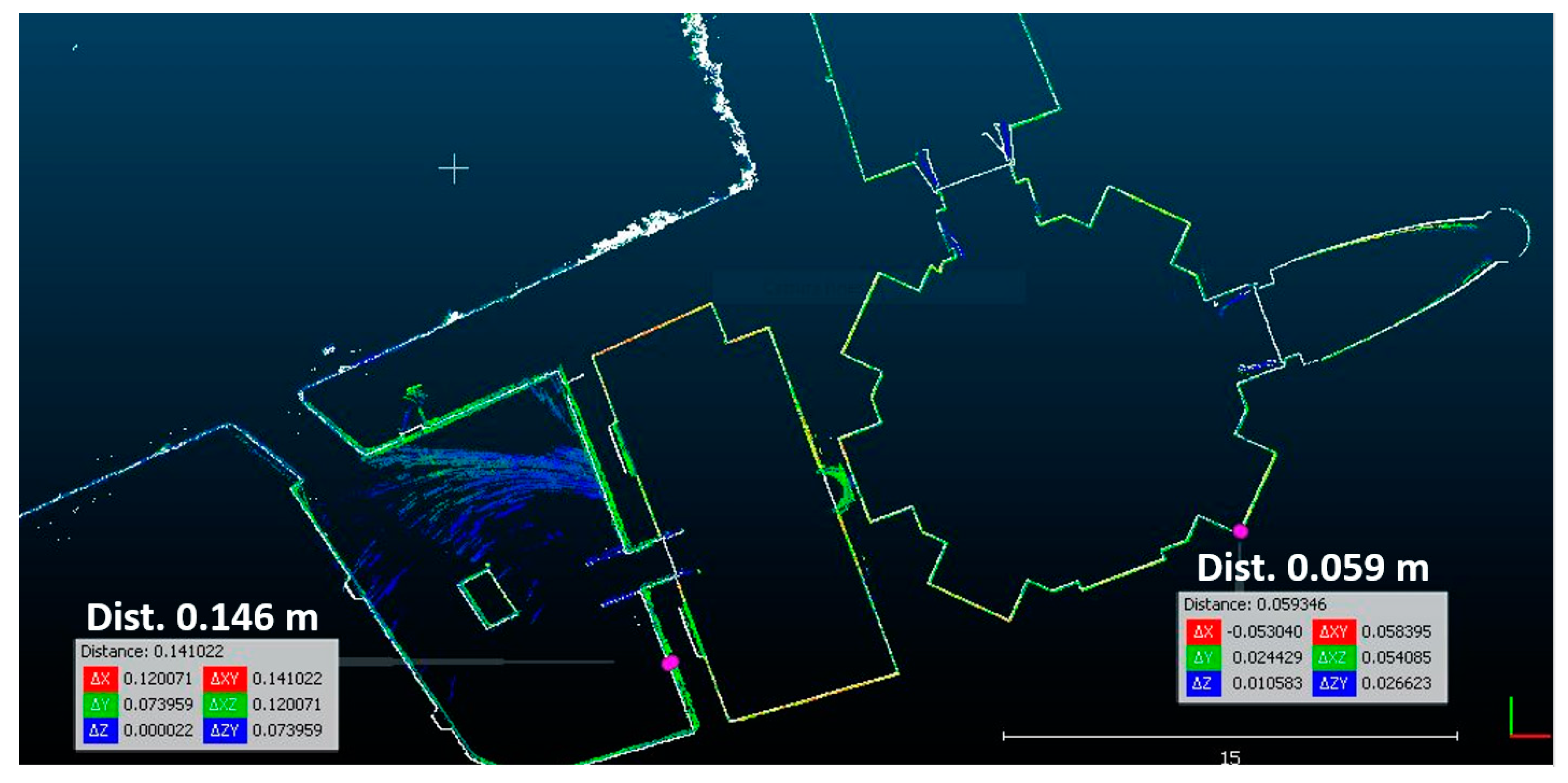
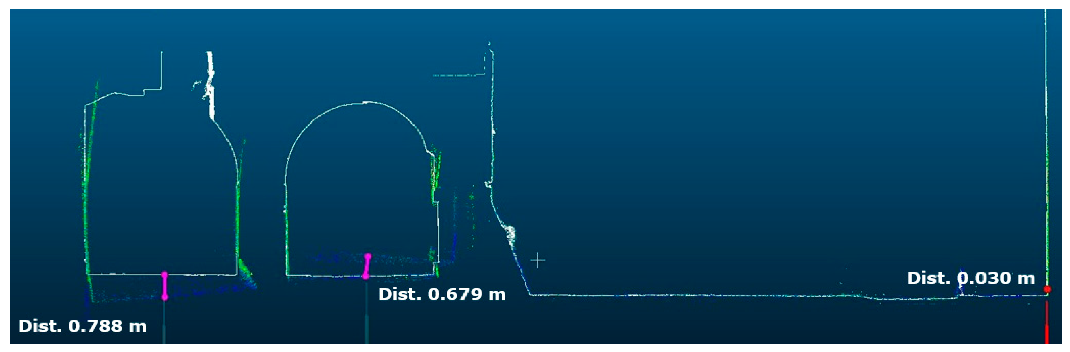
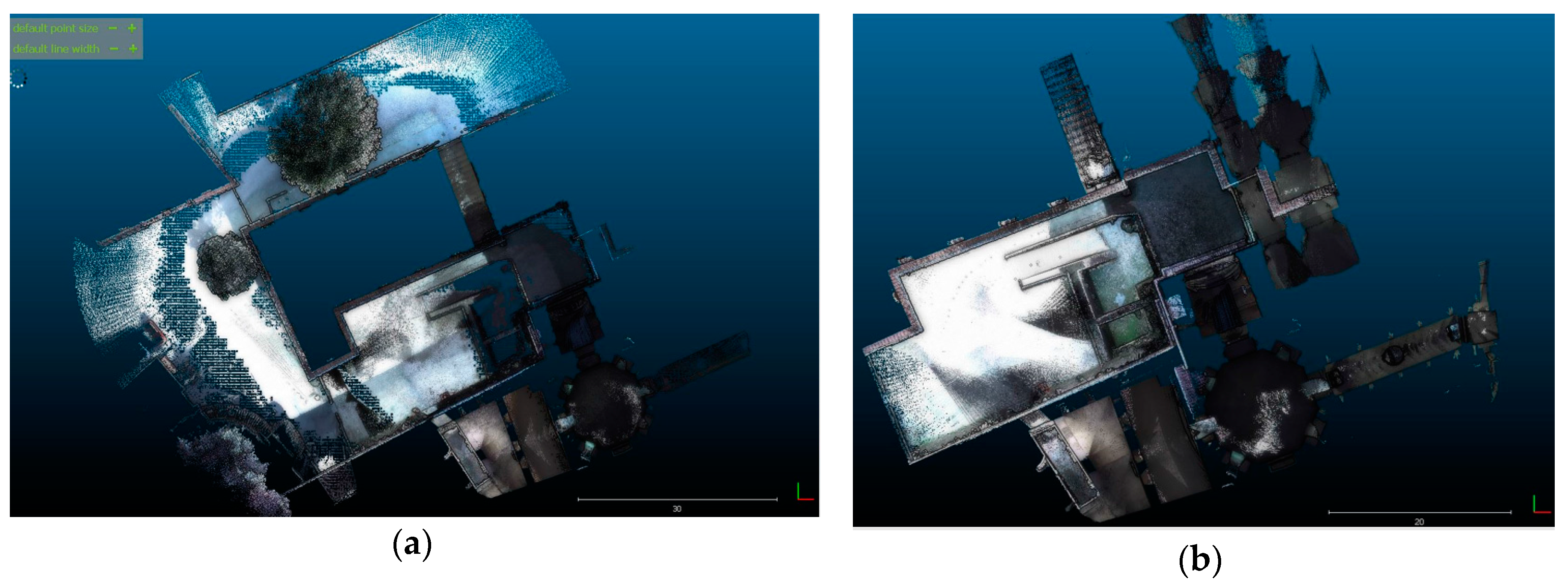
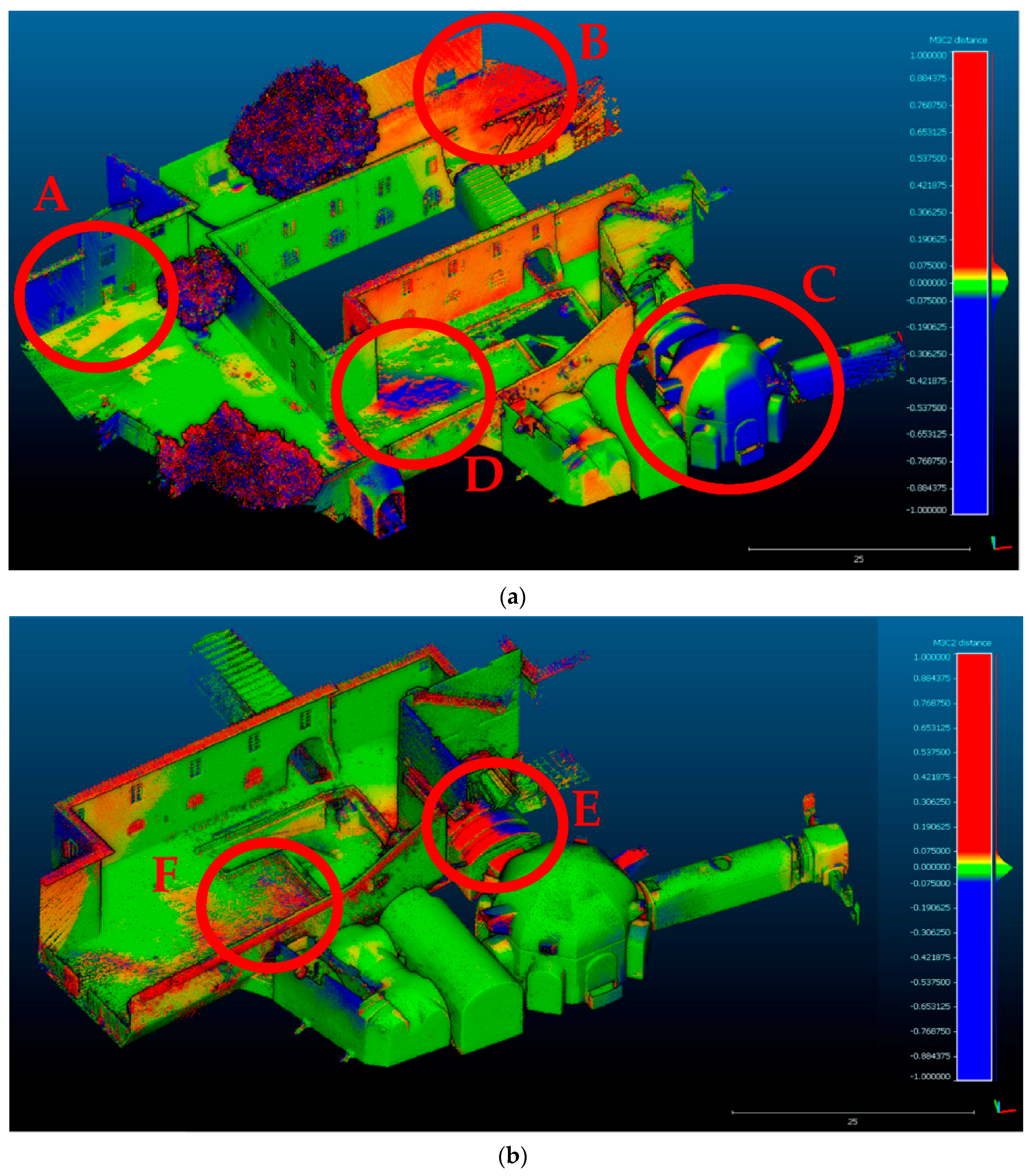
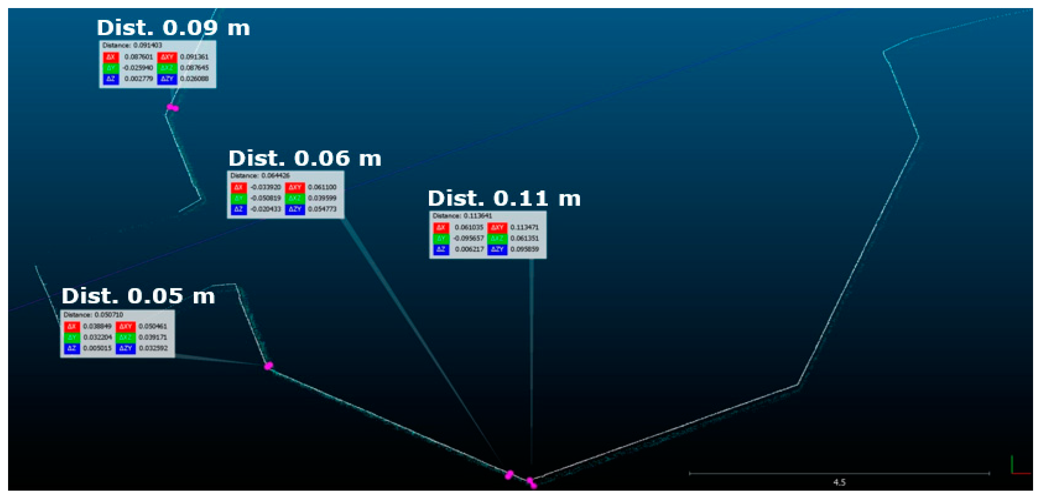
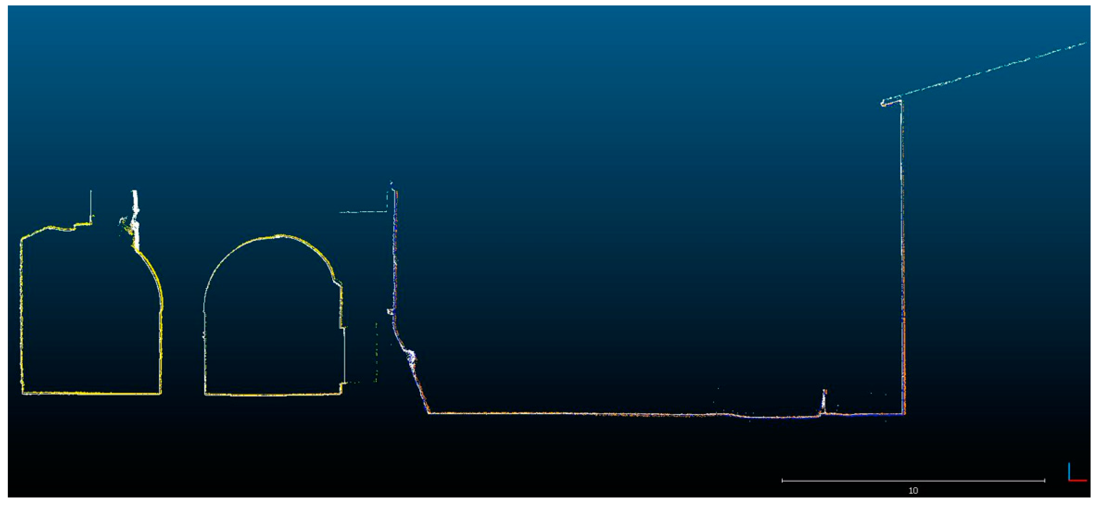
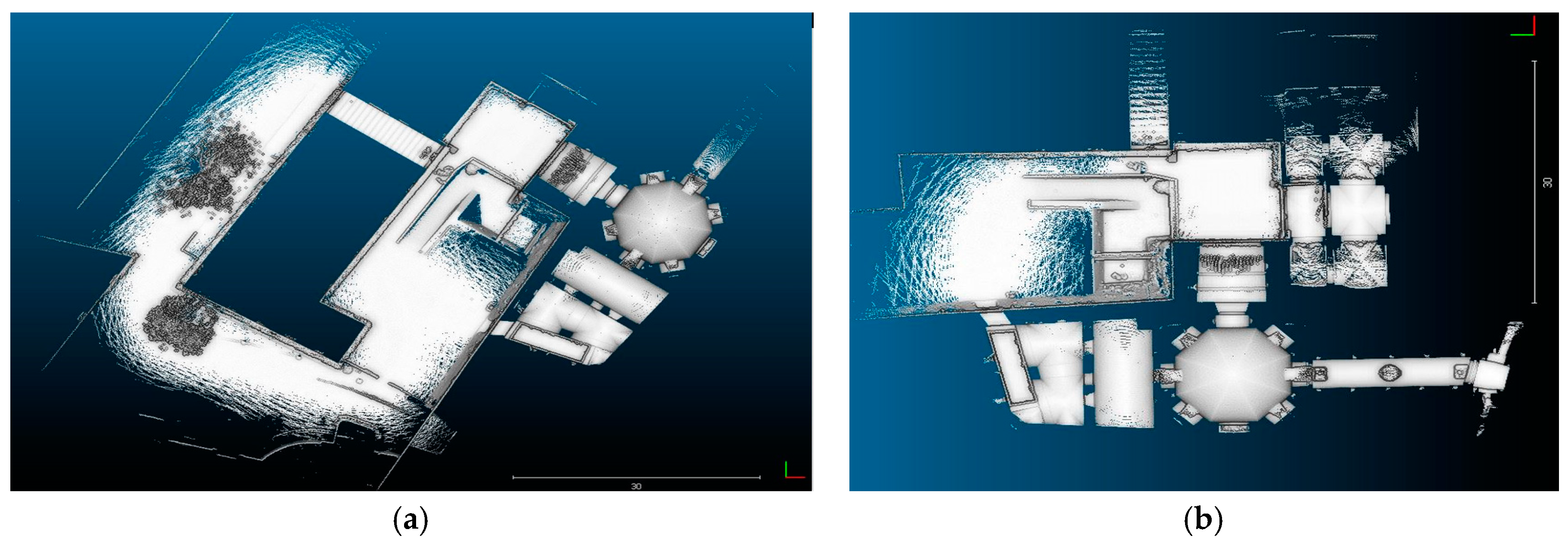


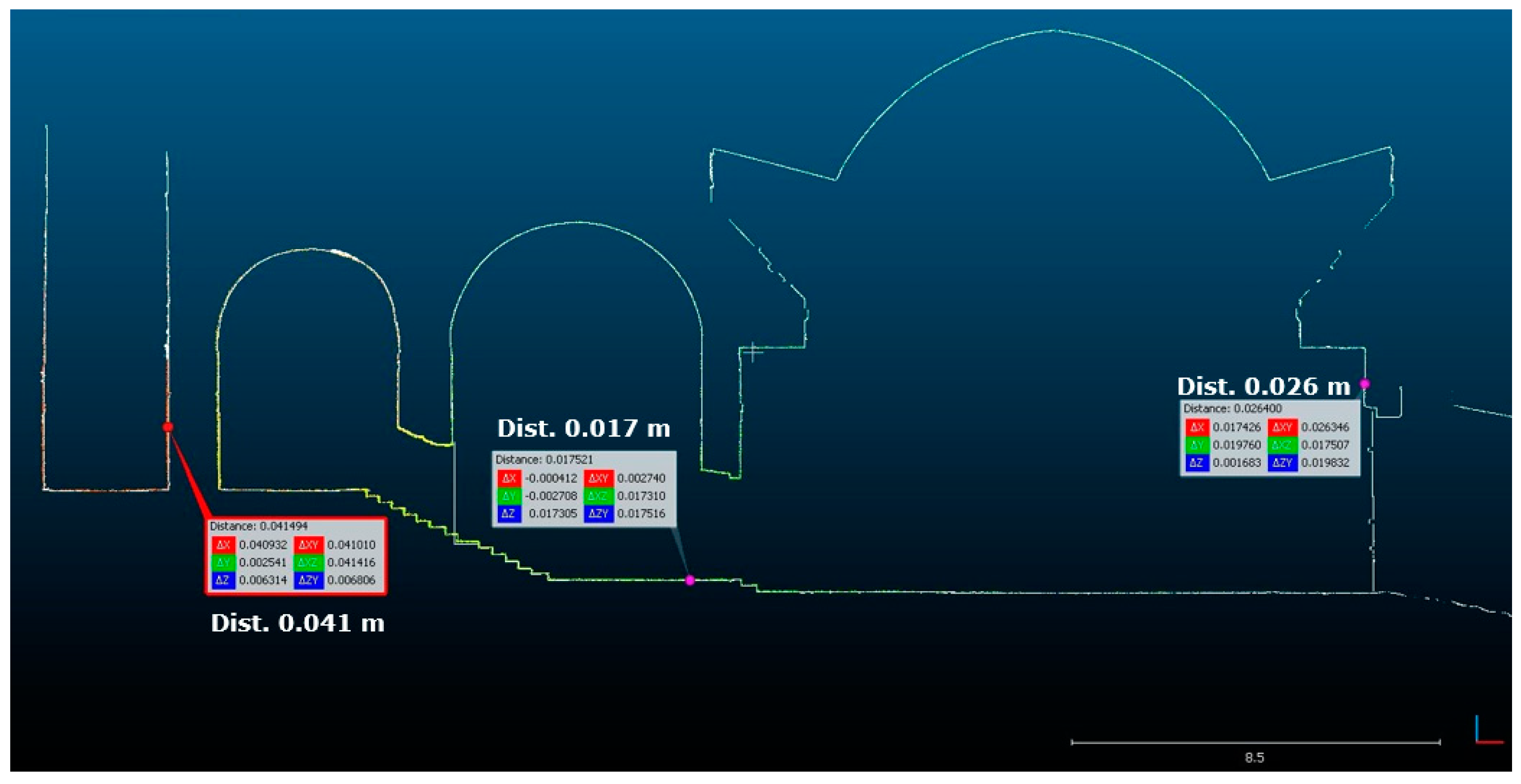
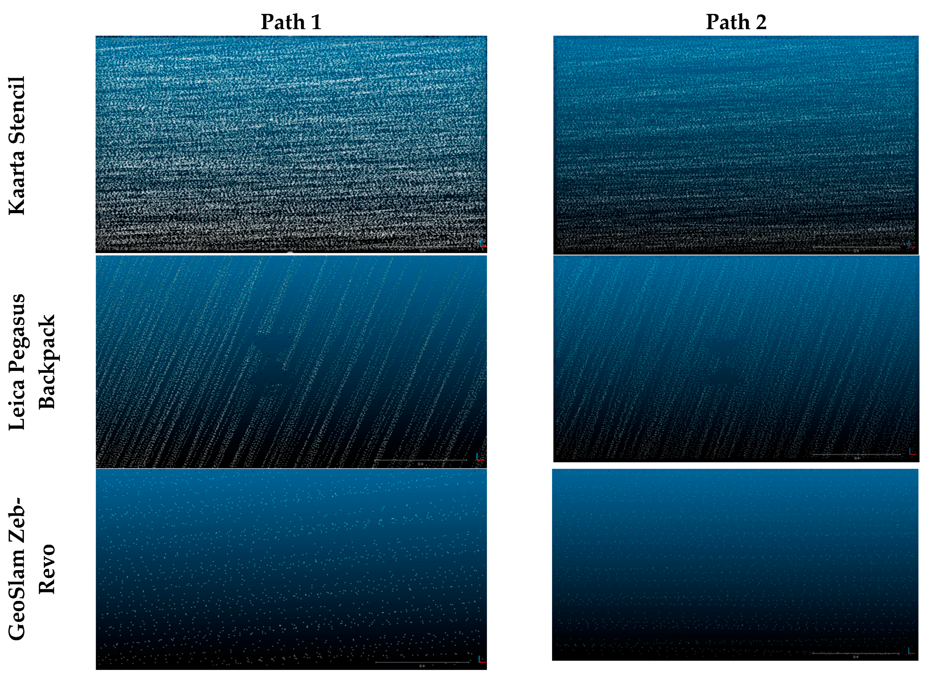
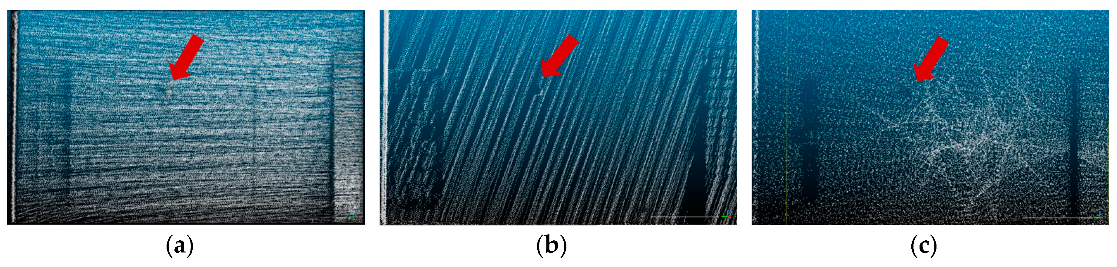
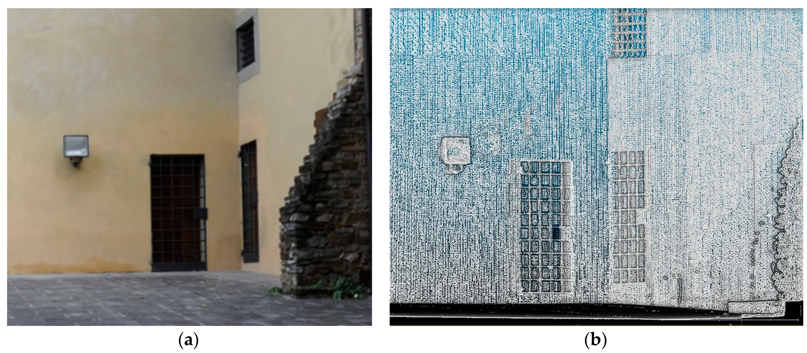
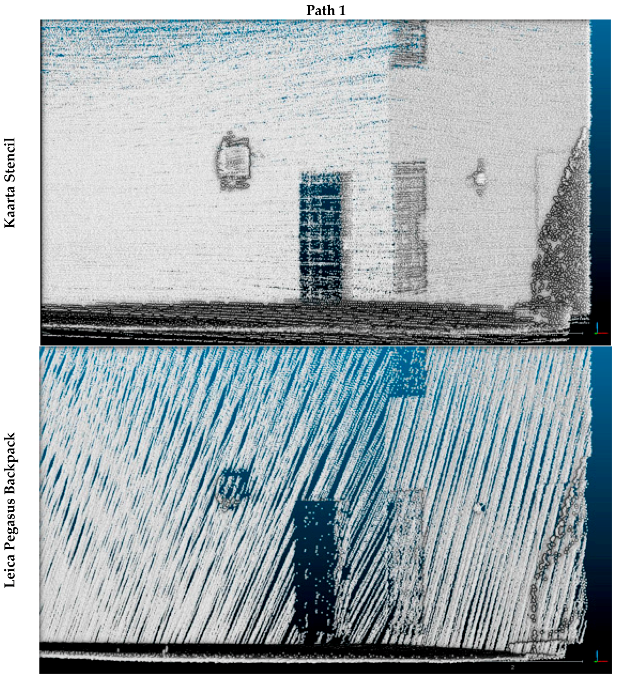
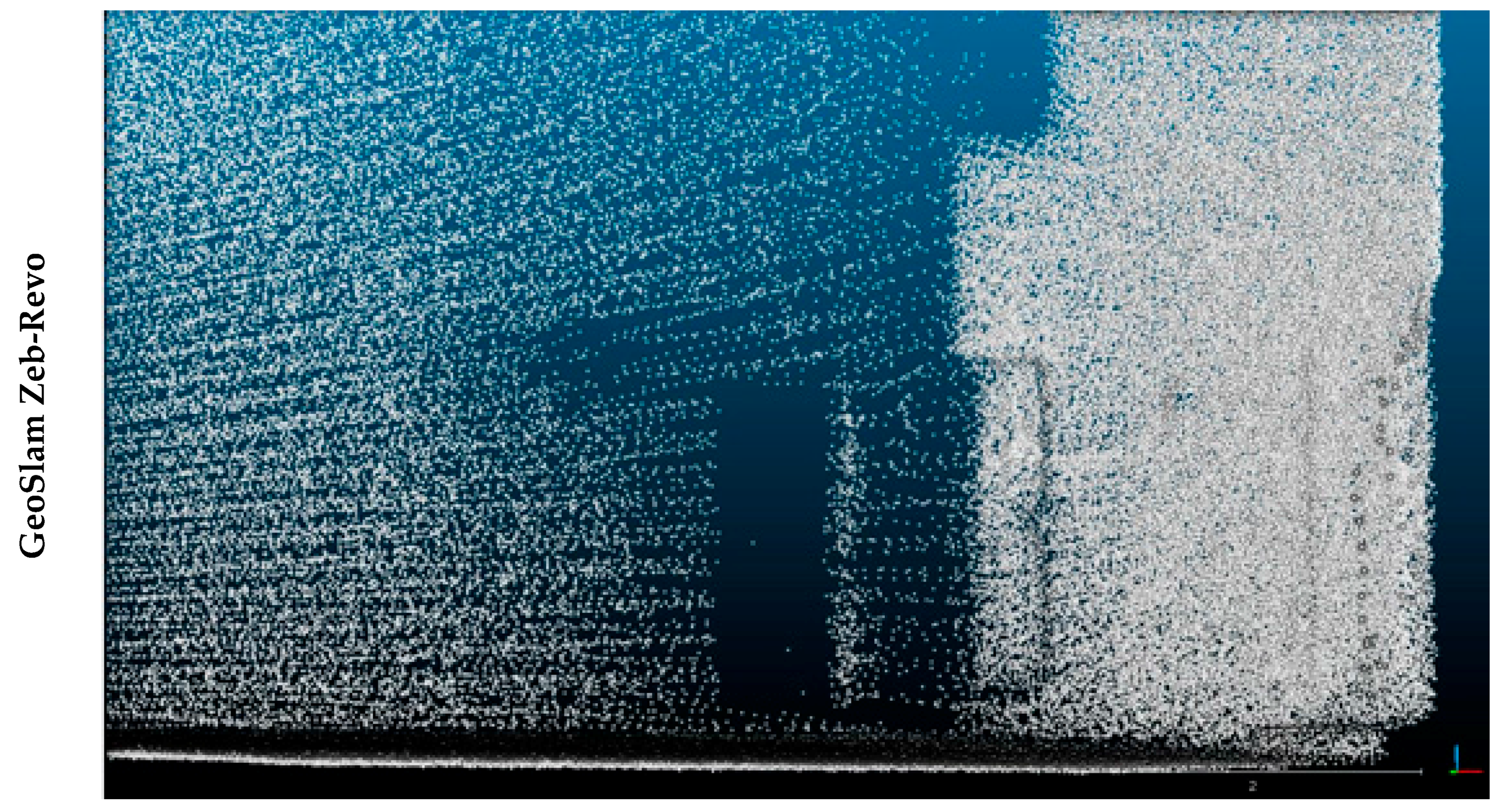
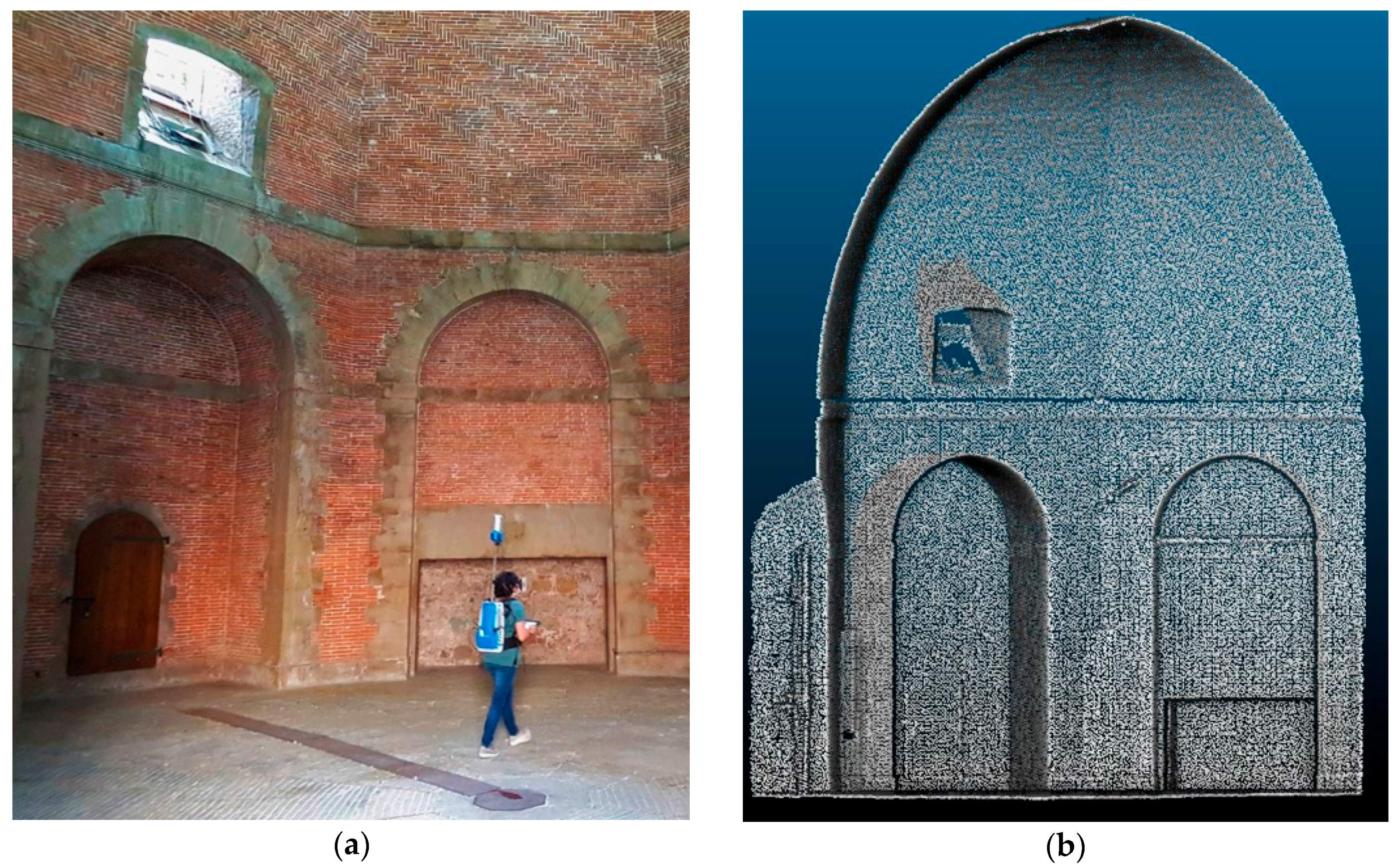
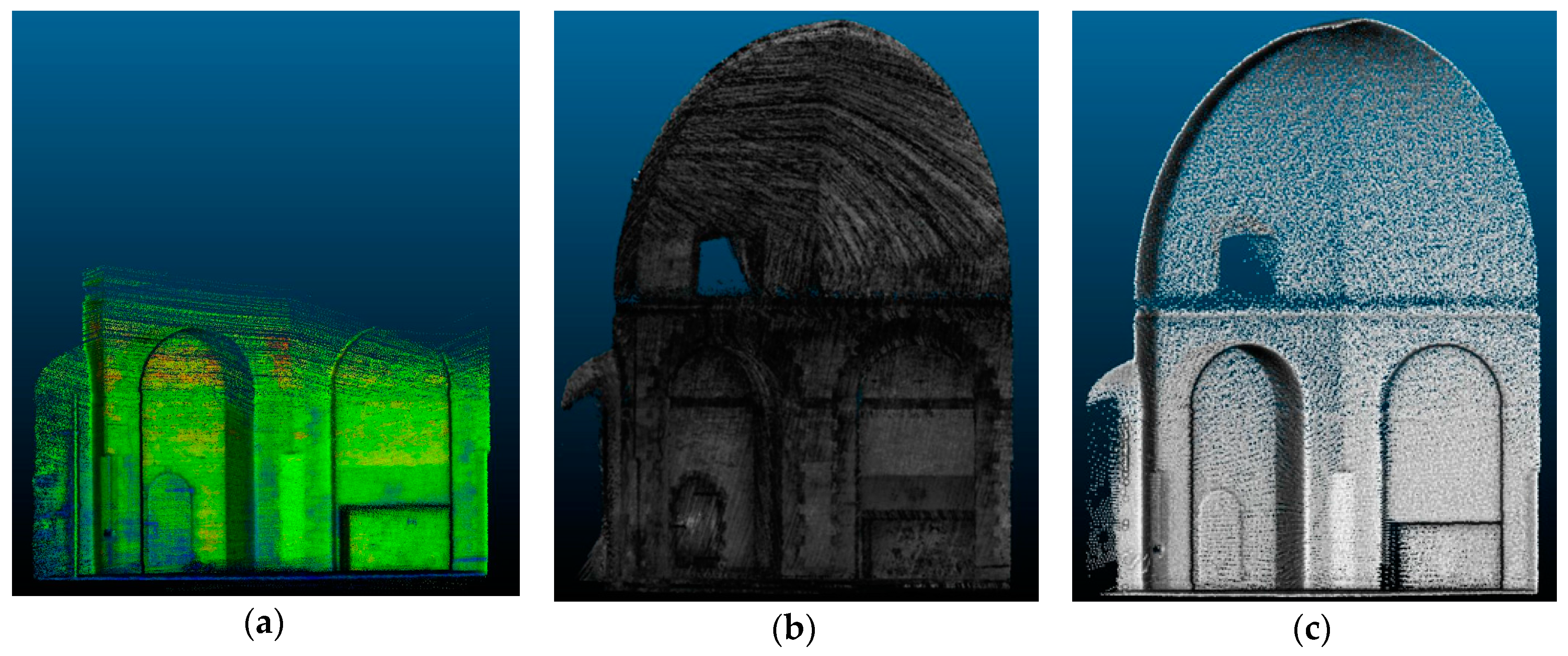

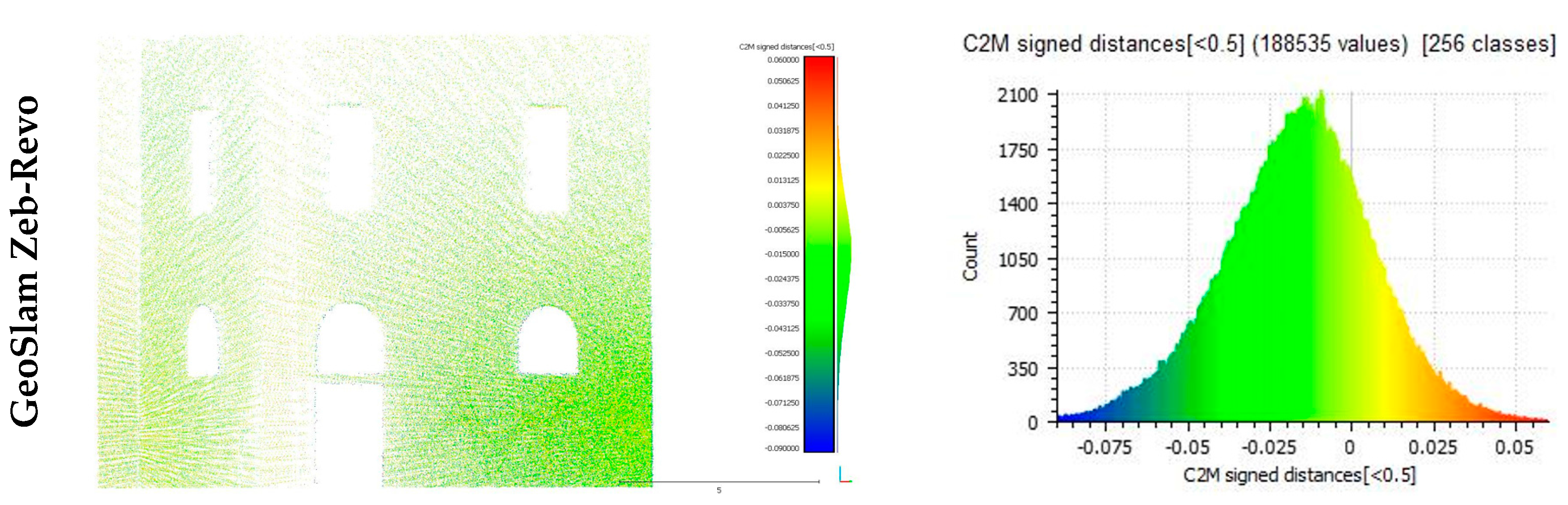
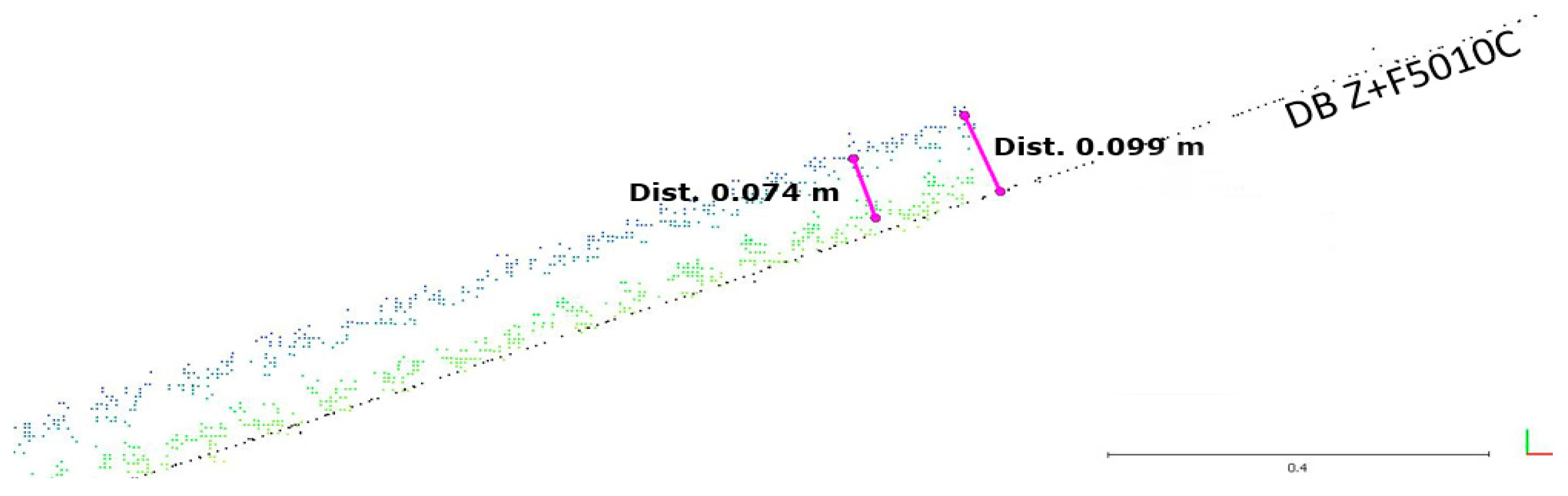
© 2018 by the authors. Licensee MDPI, Basel, Switzerland. This article is an open access article distributed under the terms and conditions of the Creative Commons Attribution (CC BY) license (http://creativecommons.org/licenses/by/4.0/).