The Effects of Drying Temperature on Nitrogen Concentration Detection in Calcium Soil Studied by NIR Spectroscopy

Abstract

Soil nitrogen is one of the crucial components for plant growth. An accurate diagnosis based on soil nitrogen information is the premise of scientific fertilization in precision agriculture. Soil nitrogen content acquisition based on near-infrared (NIR) spectroscopy shows the significant advantages of high accuracy, real-time analysis, and convenience. However, soil texture, soil moisture content, and drying temperature all affect soil nitrogen detection by NIR spectroscopy. In order to investigate the effects of drying temperature on calcium soil nitrogen detection and its characteristic bands, soil samples were detected at a 25 °C placement (ambient temperature) after 40 °C drying (medium temperature), 60 °C drying (medium-high temperature), 80 °C drying (high temperature), and 105 °C drying (extreme high temperature), respectively. Besides that, the original spectra were pretreated with five preprocessing methods, and the characteristic variables were selected by competitive adaptive reweighted squares (CARS) and backward interval partial least squares (BIPLS). The partial least squares (PLS) method was used for modeling and analysis. The predictive abilities were assessed using the coefficients of determination (R²), the root mean squared error (RMSE), and the residual predictive deviation (RPD). As a result, the characteristic bands focus on 928–960 nm and 1638–1680 nm when soil was detected after 40 °C, 60 °C, and 80 °C drying. Calcium soil obtained the best prediction accuracy $(R_p^2=0.966, RMS{E}_p=0.128\frac{\mathrm{g}}{\mathrm{kg}},RPD=5.03)$ after 40 °C drying by the method of CARS-BIPLS-PLS. Meanwhile, the prediction model also performed well when soil was detected after 60 °C drying $(R_p^2=0.946,RMS{E}_p=0.172\mathrm{g}/\mathrm{kg},RPD=4.53)$ and 80 °C drying $(R_p^2=0.961, RMS{E}_p=0.143\frac{\mathrm{g}}{\mathrm{kg}},RPD=4.98)$. However, the calcium soil obtained the worst detection result when soil was placed at 25 °C. In conclusion, a low or extremely high drying temperature had an adverse influence on the soil nitrogen detection, and the 40 °C drying temperature as well as the CARS-BIPLS-PLS method were optimal to enhance the soil nitrogen detection accuracy.

1. Introduction

Soil nitrogen is the key parameter supporting plant growth and development [1]. Thus, it is of great importance to obtain soil nitrogen information quickly and accurately for precision fertilization and agricultural production [2]. However, many conventional soil analytical techniques, such as Dumas combustion, are often complex because of the multi-component interactions [3]. The use of near-infrared (NIR) spectroscopy to estimate soil nitrogen content shows a greater advantage and prospects for wider application [4]. In recent years, many scholars have used NIR spectroscopy to detect soil nitrogen and have improved the detection accuracy with respect to soil water content removal, soil spectral data processing, characteristic bands selection, and algorithm optimization.

Firstly, NIR spectroscopy could also be used as a rapid, inexpensive, and non-destructive technique to predict some physical, chemical, and biochemical properties of soil [5]. Soil nitrogen was detected with the multiple linear regression method at spectral bands of 1702, 1870, and 2052 nm using NIR spectroscopy [6]. He et al. detected N, P, K, organic matter (OM), and pH content in a loamy mixed soil. The results showed that the correlation coefficients between the measured and the predicted values of N, OM, and pH were 0.93, 0.93, and 0.91 respectively [7]. Secondly, the effects of soil water content on soil nitrogen detection were researched. The prediction performance of carbon and nitrogen content affected by sample grinding was studied, and the results showed that the prediction accuracy was the highest with oven-dried, 0.2 mm ground soil samples [8]. Moreover, the wavelet decomposition and continuous removal methods were used to reduce the interference of soil moisture on soil total nitrogen detection by NIR spectroscopy in Zhang’s research, where both of those two methods performed well [9]. Third, the characteristic bands of soil nitrogen using NIR spectroscopy were also studied. The selected bands at 556, 1642, and 2491 nm were found to be the optimum prediction model of soil nitrogen content of black soil in Northeast China [10]. However, Shi et al. proposed that the 1450, 1850, 2250, 2330, and 2430 nm bands could be selected as the characteristic bands to estimate organic nitrogen content in soil based on visible NIR spectroscopy [11]. Besides, the 1902, 2364, 1826, and 2098 nm bands were selected as the characteristic bands to predict soil nitrogen using NIR spectroscopy in He’s research [12]. The determination coefficient of soil total nitrogen prediction reached 0.94 using the characteristic bands of 1100 and 2300 nm with the partial least squares regression(PLSR) model [13].

Moreover, temperature also affects soil nitrogen detection by NIR spectroscopy [14]. Particularly, drying temperature has an influence on water removal and the activity of urease [15]. The effects of soil water content on soil nitrogen detection by NIR spectroscopy have been studied a lot, while the effects of drying temperature on the detection of nitrogen by NIR spectroscopy have seldom been studied. In the current studies, drying is generally used to remove soil moisture but the optimum drying temperature was rarely considered. Coarse samples were dried at 20 °C for 48 h for the prediction of C and N content using visible near-infrared spectroscopy, and the comparative method was used to detect their potential mineralization in heterogeneous soil samples [16]. Flat-dry samples were dried at 35 °C for 12 h to explore the effects of soil sample pretreatments and standardized rewetting [17]. Soil was subjected to oven drying at 60 °C for 24 h, after which it was ground and sieved with a 0.002 m sieve [18]. Soil samples were dried at 80 °C for 8 h to detect soil nitrogen with different pretreatments using an NIR sensor in He’s research [19,20]. Besides this, soil samples were dried at 95 °C for 24 h and then sieved for estimating total nitrogen using NIR [21]. Soil samples were also dried naturally, rolled, broken into pieces, and then sieved with a 2 mm screen for estimating the organic matter and nitrogen [22,23]. However, the impacts of drying temperature on soil nitrogen detection have been studied little and the effect mechanism is not clear yet.

According to the current studies mentioned above, the objective of this study was to investigate the influence of drying temperature on soil nitrogen detection in calcium soil and its characteristic bands. Meanwhile, the mechanism of drying temperature for soil nitrogen detection by NIR spectroscopy from the perspective of preprocessing methods, soil properties, and characteristic bands was also researched.

2. Materials and Methods

2.1. Experimental Materials and Sample Preparation

The calcium soil whose nitrogen content is around 0.5 g/kg to 3 g/kg was selected as the experimental material, which was collected from Jining (35°23′ N, 116°33′ E, Shandong province, Jining, China). It contains a certain amount of organic matter and ash with a loose soil texture. This region belongs to a monsoon climate of medium latitudes, whose mean temperature is 13.3–14.1 °C and whose average annual rainfall is 597–820 mm. The soil samples’ preparation process was as follows. First, the soil samples were sieved with a 40 mesh sieve (0.425 mm) and grinded. Second, urea solutions with different concentrations were prepared and mixed with soil samples. The detected nitrogen concentration gradients ranged from 0.5 to 2.5 g/kg (11 nitrogen gradients were set with 16 samples for each gradient, 176 soil samples for each drying temperature). Meanwhile, the soil samples without urea added were used as references. Third, the experiments were carried out in five groups. The soil samples in four groups were dried at 40 °C for 48 h, 60 °C for 24 h, 80 °C for 18 h, and 105 °C for 12 h, respectively, to fully eliminate the water in the soil, which avoided the influence of soil water on NIR detection. The soil samples in the last group were dried and then placed at 25 °C for 10 days. Considering that the moisture in the air might be absorbed by the soil samples, the soil water content was measured before detection.

2.2. NIR Spectrum Collection

Near-infrared light is an electromagnetic wave between infrared and visible light. The spectral information originates from the vibration of the O–H, C–H, and N–H groups, which can reflect the variety of organic matter in the characteristic signal of the spectral region [24]. The portable NIR optical instrument used in this experiment is from Isuzu Optics Corp (Shanghai, China), which is an interferometer instrument that is reflective with two integrated tungsten halogen lamps. The instrument collects spectral information in the 900–1700 nm acquisition range, and its optical resolution is 10 nm. Before performing the spectroscopic measurement, the instrument should be preheated for 15 min and be prepared with a blackboard and whiteboard correction operation. The spectral acquisition parameter is set up with 400 points, and the spectra is obtained by averaging three scans. In this study, the spectra were recorded and modeled in reflectance mode.

2.3. Spectral Preprocessing Methods

In this study, in order to reduce the spectral noise, baseline drift, and the interference from other backgrounds as well as distinguish overlapping peaks, five preprocessing methods were applied to improve spectral resolution, sensitivity, and the signal-to-noise ratio of the spectra [25]. Among them, the Savitzky–Golay (S–G) smoothing algorithm uses a weighted average method to quantize the data in the moving window by polynomial least squares fitting as well as emphasizes the central role of the center point [26]. The basic idea of the multiplicative scatter correction (MSC) algorithm is to use an ideal spectrum to represent all spectra linearly regressed with the sample spectra, and the original spectra is corrected with the slope and intercept of the linear equation [27]. The principle of the standard normal variation (SNV) algorithm is that the absorbance value of each wavelength point satisfies a certain distribution in each spectrum, and the spectral correction is performed according to this assumption [28]. The idea of the detrending (DT) algorithm is that the spectral absorbance and wavelength are first fitted into a trend line d according to the polynomial, and then the trend line d is subtracted from the original spectra x to achieve the effect of the trend [29]. The 1st-Derivation (1st-Der) method can distinguish the overlapping peaks and eliminate interference from other backgrounds, which improves spectral resolution, sensitivity, and the signal-to-noise ratio of the spectra.

2.4. Characteristic Variable Selection Method

The characteristic variable selection method, also called attribute selection or variable selection, refers to the selection of input variables with the greatest predictive power for a particular output requirement.

2.4.1. Competitive Adaptive Reweighted Sampling

The competitive adaptive weighted algorithm method, which imitates the evolution of the “survival of the fittest” principle, phases out of the invariable wavelength. It uses the Monte Carlo sampling method or the random sampling method to select a part of the sample from the calibration set for partial least squares (PLS) modeling and repeats this process for hundreds of iterations. The algorithm chooses part of the samples in the total sample set to carry out PLS modeling. In the process of wavelength variable selection, only the wavelength variables with a large absolute value of the PLS regression coefficient are kept, while the wavelength variables with a small absolute value of PLS regression coefficients are removed. Thus, a part of the optimal wavelength variable subset is obtained [30].

2.4.2. Backward Interval Partial Least Squares (BIPLS)

BIPLS is a variable selection method mainly used to filter the wavelength range of a PLS model and reduce the amount of sub-intervals of the worst or collinear variables, which select the best principal component number according to the root mean square error of cross validation (RMSECV) [31,32]. The algorithm steps are mainly as follows:

a. Divide the whole spectrum into k bands of equal width. b. Leave a section from the k section spectrum. Carry out the PLS regression on the remaining (k − 1) section and establish the sub model of the quality to be measured. Set aside each paragraph in turn to get the k sub model. c. Measure the accuracy of each model by the RMSECV value. Delete the reserved segment corresponding to the highest precision sub-model, and take the sub-model as the first base model. d. Leave one more section in the remaining (k − 1) section of the spectrum and use the remaining (k − 2) segments to model the PLS. Each section is set aside in order to obtain the (k − 1) sub-model to remove the reserved segments corresponding to the sub-model of the minimum RMSECV value. Take the sub-model as the second base model. Repeat the process for the remaining wave bands. e. Investigate the (the prediction root mean square error) RMSEP value of each base model according to steps b to d. Select the best and minimum RMSECV among all the base models, and the corresponding interval combination is the best combination.

2.5. Modeling Method

Partial least squares (PLS) is a commonly used multivariate statistical method, which extracts the most comprehensive variables and identifies the noise by decomposing and filtering the data in the system [33,34]. In the PLS model, the spectral matrix is decomposed first and the main principal component variables are obtained. Then, the contribution rate of each principal component is calculated. Based on the accumulative contribution rate of principle components, the principal components are selected as input to establish a mapping relationship with chemical indicators. Generally, the flexibility of PLS makes it possible to establish a regression model in the case that the number of samples is less than the number of variables [35].

2.6. Model Evaluation Index

In this experiment, the modeling effect is evaluated by the coefficient of determination (R²), the root mean square error (RMSE), and the residual predictive deviation (RPD). The coefficient of determination R² reflects the level of intimacy between variables, the RMSE reflects the accuracy of the model, and the RPD reflects the prediction ability of the model. The higher the RPD, the lower the RMSE, and the closer the R² is to 1, the better the performance of the prediction model. In this paper, $R_c^2$ and $R_p^2$ represent the coefficient of determination of the calibration set and the prediction set, respectively, and $RMS{E}_c$ and $RMS{E}_p$ represent the root mean square error of the calibration set and prediction set, respectively. Besides this, the RPD has been suggested to be at least 3 for agriculture applications; where 2 < RPD < 3 indicates a model with a good prediction ability; 1.4 < RPD < 2 is an intermediate model needing some improvement; and RPD <1.4 indicates that the model has a poor prediction ability [36].

3. Results and Discussion

3.1. Temperature and Soil Reflectance

In this experiment, the spectra of calcium soil at five drying temperatures were collected. Figure 1 shows the raw spectra and the other five pretreated average spectra when soils were detected after 40 °C drying. The abscissa of the curve is the wavelength and the ordinate of the curve is the average spectral reflectance in Figure 1a–c.

Figure 1a shows the raw spectra and Figure 1b shows the spectra after S–G smoothing pretreatment. With the increase of nitrogen concentration in the soil, the spectral reflectance of the soil decreases gradually, that is, the spectral absorbance of the soil increases gradually, which conforms to the Lambert–Beer law [37]. The spectral reflectance of the calcium soil decreases gradually near 1400 nm, which is caused by the vibration of O–H, and similar results also occurred in Shi et al.’s research [11]. Figure 1c shows the spectra after MSC processing and Figure 1d shows the spectra with SNV pretreatment. These two methods make the different concentrations’ average spectra concentrated, but the spectral reflectance still decreases obviously around 1400 nm. It is clear that the DT-treated soil spectra near 1650–1680 nm has a more obvious decline trend in Figure 1e. Figure 1f shows the spectra after 1st-Der processing, and the spectral resolution is increased. There is a large fluctuation around 1650 nm and a similar result can be found in Dalal’s research [5].

The relationship between drying temperatures and soil reflectance is further investigated and analyzed. Figure 2 shows the raw average spectra of different drying temperatures when the soil nitrogen concentration is 2.5 g/kg.

According to Figure 2, with the increase of drying temperature, the reflectance strength of the spectra decreases gradually, indicating that the higher the drying temperature, the lower the spectral reflectance strength. Moreover, as the drying temperature increases, the soil spectral reflectance shows a decreasing trend around 1100 nm. The reason might be that medium and high temperature could stimulate the activity of soil urease as well as remove the influence of soil water [38]. Thus, the N–H bonds vibrate more obviously than the O–H bands.

3.2. Full-Waveband Data Analysis and Modeling

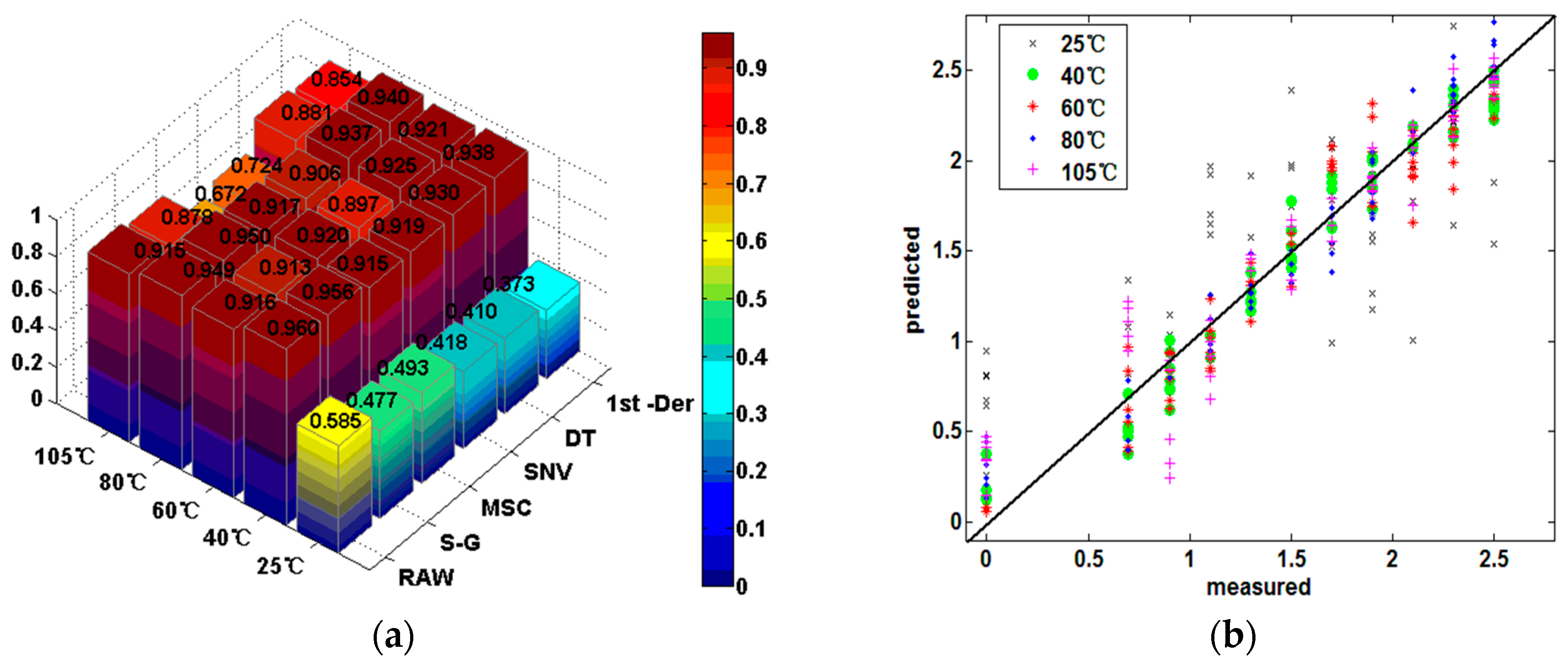
In this experiment, soil samples were divided into the calibration set and the prediction set according to the ratio of 2:1 using the (sample set partitioning based on joint x–y distance) SPXY method [39]. The raw spectra and the other five pretreated spectra were modeled and analyzed by PLS.

Table 1. The prediction effects with different spectral pretreatments and different drying temperatures by the partial least squares (PLS).

Methods	Group	Calibration Set		Prediction Set			N
		$R_c^2$	RMSECV (g/kg)	$R_p^2$	RMSEP (g/kg)	RPD
RAW	25 °C	0.639	0.315	0.585	0.483	1.46	6
	40 °C	0.959	0.102	0.960	0.148	4.88	6
	60 °C	0.956	0.112	0.916	0.197	3.29	7
	80 °C	0.955	0.105	0.949	0.170	4.67	7
	105 °C	0.936	0.122	0.915	0.231	3.42	6
S–G	25 °C	0.856	0.193	0.477	0.541	1.37	9
	40 °C	0.962	0.097	0.956	0.171	4.31	6
	60 °C	0.972	0.086	0.913	0.203	3.32	9
	80 °C	0.954	0.105	0.950	0.172	4.36	7
	105 °C	0.943	0.114	0.878	0.285	2.83	8
MSC	25 °C	0.803	0.256	0.493	0.480	1.03	8
	40 °C	0.964	0.092	0.915	0.184	3.45	6
	60 °C	0.924	0.146	0.920	0.195	3.42	5
	80 °C	0.986	0.059	0.917	0.207	3.47	10
	105 °C	0.963	0.096	0.672	0.276	1.49	10
SNV	25 °C	0.898	0.183	0.418	0.544	0.89	10
	40 °C	0.962	0.092	0.919	0.184	3.62	6
	60 °C	0.928	0.144	0.897	0.221	2.92	5
	80 °C	0.992	0.044	0.906	0.219	3.25	12
	105 °C	0.931	0.129	0.724	0.233	1.75	8
DT	25 °C	0.756	0.274	0.410	0.487	1.28	7
	40 °C	0.972	0.085	0.930	0.178	3.80	7
	60 °C	0.953	0.109	0.925	0.211	3.51	7
	80 °C	0.979	0.071	0.937	0.187	3.99	9
	105 °C	0.857	0.202	0.881	0.222	2.89	7
1-Der-	25 °C	0.773	0.250	0.373	0.575	1.24	7
	40 °C	0.982	0.066	0.938	0.202	3.79	8
	60 °C	0.922	0.146	0.921	0.205	3.25	5
	80 °C	0.986	0.060	0.940	0.181	4.03	10
	105 °C	0.848	0.212	0.854	0.246	2.50	3

RMSECV: root mean square error cross validation; RPD: residual predictive deviation.

and Figure 3a present the prediction results under different drying temperatures using different preprocessing methods.

First, when soil samples were detected after 40 °C, 60 °C, and 80 °C drying, the soil nitrogen detection accuracy ($0.879<R_p^2<0.960,0.221\mathrm{g}/\mathrm{kg}<RMS{E}_p<0.148\mathrm{g}/\mathrm{kg},2.92<RPD<4.88$) are better than that of 25 °C placement and 105 °C drying. However, soil nitrogen detection was the worst ($0.373<R_p^2<0.585,0.483\mathrm{g}/\mathrm{kg}<RMS{E}_p<0.573\mathrm{g}/\mathrm{kg},1.24<RPD<1.46$) when soils were placed at 25 °C. Meanwhile, the detection effects ($0.672<R_p^2<0.915,0.276\mathrm{g}/\mathrm{kg}<RMS{E}_p<0.231\mathrm{g}/\mathrm{kg},1.49<RPD<3.42$) are not stable when the drying temperature is 105 °C. The reason might be that medium and high temperature could largely remove the soil water, but an extremely high drying temperature would destroy the soil urease activity as well [38]. Meanwhile, little soil water content was preserved (water content: 3.6%) when soils were placed at 25 °C for a long time. Compared with the O–H bonds in water, the N–H bonds exist mostly in the form of multiple frequency or combination frequency. Thus, the N–H bonds are relatively weak for extracting soil nitrogen information in soil [40].

Second, from the aspects of the preprocessing methods with PLS, the ranking of prediction effects is RAW > S–G > DT > 1st-Der > SNV > MSC. In general, the spectra with suitable pretreatments could improve the accuracy of modeling and prediction to a certain extent. However, since the NIR spectra have no obvious characteristic peaks or fingerprint peaks, the pretreated methods might remove some useful information of the raw spectra, which causes the problem of spectral signal distortion. Among them, the spectral preprocessing methods of MSC and SNV might have the problem of spectral over-correction. Besides this, 1st-Der is very sensitive to a high-frequency signal but meanwhile it may ignore some useful spectral information [26,27].

Figure 3b displays the PLS prediction results of raw spectra dealing with different temperatures. The X-axis is the soil nitrogen content and the Y-axis is the predicted soil nitrogen content. It is suggested that the fitting effects are better when the soil is detected after 40 °C, 60 °C, and 80 °C drying than that of a 25 °C placement and 105 °C drying. Additionally, the fitting effect is the worst with the soil at a 25 °C placement, which is consistent with the predicted R² value.

3.3. Sensitive Wavebands Selection

In this paper, the competitive adaptive reweighted squares (CARS) algorithm was used to select the characteristic variables of NIR spectra. Meanwhile, the BIPLS algorithm was used for selecting the characteristic intervals. The selection process of characteristic variables and characteristic intervals after 40 °C soil drying is taken as an example in the following.

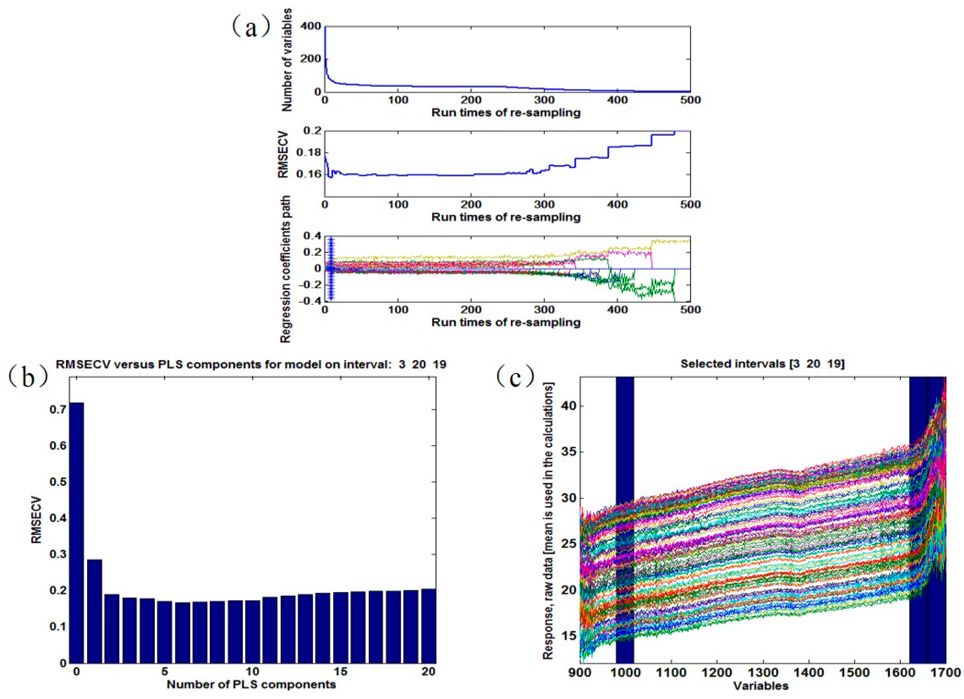
Figure 4a displays the selection process of characteristic variables carried out by CARS. In the CARS algorithm, the sampling times were set as 500. The variables were selected by attenuation functions during each iteration, but only the wavelength variables with large absolute values of PLS regression coefficients were preserved. In this experiment, the CARS algorithm was operated for 10 times for each temperature, and characteristic variables that occurred more than 6 times were selected as the final characteristic variables. The specific steps of the algorithm can be found in the reference [20].

Figure 4b shows the selection process of the characteristic intervals of soil spectra by BIPLS and Figure 4c presents the best principle numbers determined by leave-one-out cross validation.

Table 2. The variable selection results of BIPLS when the spectra with 400 points are divided into 20 segments.

Int-Number	Interval-ID	RMSECV	Number of Variables	Int-Number	Interval-ID	RMSECV	Number of Variables
20	1	0.174	400	10	4	0.168	200
19	18	0.173	380	9	8	0.167	180
18	17	0.172	360	8	11	0.167	160
17	16	0.172	340	7	5	0.167	140
16	14	0.171	320	6	6	0.167	120
15	13	0.170	300	5	2	0.167	100
14	15	0.170	280	4	7	0.166	80
13	12	0.170	260	3	3	0.167	60
12	9	0.169	240	2	20	0.169	40
11	10	0.168	220	1	19	0.226	20

lists the variable selection results of BIPLS when the spectra with 400 points are divided into 20 segments. As the spectral interval is gradually removed, the RMSECV value of the model changes continuously, and the number of remaining intervals and variables in the model decreases at the same time. As can be seen in Table 2, when the spectral interval numbered 4 is eliminated, the RMSECV of the model reaches a minimum 0.166. The remaining three intervals in the model are the range of the final participation. The selected interval numbers are 3, 20, and 19.

Table 3. The selected characteristic variables, characteristic intervals, and sensitive wavebands.

Group	CARS Algorithm		BIPLS Algorithm
	Characteristic Variables (nm)	Number	Characteristic Intervals (nm)	Serial Number of Characteristic Interval
25 °C	1614 1626 1647 1649 1651 1664 1666 1668 1669	9	1036–1078, 1633–1666	4, 19
40 °C	1638 1640 1642 1644 1669 1671 1673 1677 1678 1680	10	991–1034, 1633–1666	3, 19
60 °C	928 933 1559 1605 1656 1661 1669 1671 1673 1675	10	1080–1022, 1598–1631, 1633–1666	5, 18, 19
80 °C	940 942 1644 1669 1671	10	1450–1486, 1524–1559	14, 16
105 °C	958 1141 942 1644	5	901–944, 1633–1666	1, 19

presents the characteristic variables and characteristic intervals, respectively. On the one hand, it can be seen that the characteristic variables selected by CARS are not same at different drying temperatures. The characteristic variables are mainly concentrated in the range of 1610–1650 nm and 1660–1670 nm when the soil was detected at 25 °C, and the characteristic variables changes when the soil was dried after 40 °C (1638–1650 nm, 1670–1680 nm). Compared with the characteristic variables, however, the characteristic intervals in BIPLS are mainly distributed at 991–1034 nm, 1036–1078 nm, and 1633–1666 nm. Besides this, when the drying temperatures rose to 60 °C, 80 °C, and 105 °C, the characteristic variables are mainly distributed in 930–950 nm and 1600–1670 nm, while the interval of the characteristic variables is mainly distributed in 991–1022 nm and 1524–1666 nm.

According to the Beer–Lambert law, the NIR spectra vary a lot because of the variation of sample components and structure [37]. Therefore, the drying temperature does affect the soil nitrogen characteristic variables based on the soil properties, and the greater the temperature differs, the greater the differences among characteristic variables. Moreover, although the selected characteristic variables are different to some extent due to the different algorithm principles of CARS and BIPLS [30,31,32], the overlap characteristic variables are mainly distributed at 1630–1680 nm and around 930 nm.

When the characteristic variables and characteristic intervals were selected, the linear correlation analysis was performed for each characteristic variable and each characteristic interval. The characteristic variables are sorted by correlation coefficients from the highest to the lowest. Finally, the characteristic variables with high correlation were selected according to the principle of the best prediction effect with the least number of variables. The final characteristic variables and the prediction performance are shown in

Table 4. The characteristic variables and prediction effects of CARS-BIPLS-PLS.

Group	Number	Characteristic Bands	${\mathit{R}}_{\mathit{c}}^2$	RMSEC (mg/kg)	${\mathit{R}}_{\mathit{p}}^2$	RMSEP (mg/kg)	RPD
25 °C	9	1614 1626 1647 1649 1651 1664 1666 1668 1669	0.738	0.428	0.728	0.408	2.01
40 °C	10	1638 1640 1642 1644 1669 1671 1673 1677 1678 1680	0.974	0.132	0.966	0.128	5.03
60 °C	10	928 933 1559 1605 1656 1661 1669 1671 1673 1675	0.951	0.181	0.946	0.172	4.53
80 °C	10	940 942 1644 1669 1671	0.966	0.152	0.961	0.143	4.98
105 °C	5	958 1141 942 1644	0.917	0.242	0.903	0.227	3.37

.

According to Table 4, the prediction effects of soil nitrogen by the method of CARS-BIPLS-PLS achieved good results when soils were detected (4.53 < RPD < 5.03, $0.946<R_p^2<0.966,0.172 \mathrm{g}/\mathrm{kg}<RMS{E}_p<0.128\mathrm{g}/\mathrm{kg}$) after 40 °C, 60 °C, and 80 °C drying. Additionally, the corresponding characteristic bands focus on 928–960 nm and 1638–1680 nm. Compared with the full spectrum model by PLS, the prediction of the characteristic bands by CARS-BIPLS-PLS is obviously better than that in the condition when the soil was detected at a 25 °C placement. The reason might be that the vibration of N–H was covered by little soil water content in the full spectrum [40]. However, the most optimal characteristic variables were selected with combined CARS and BIPLS and the noise information was also removed [30,31,32].

3.4. Comparison of Results

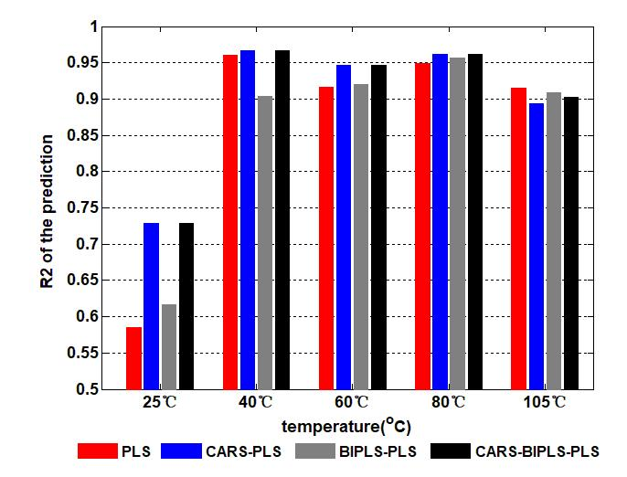
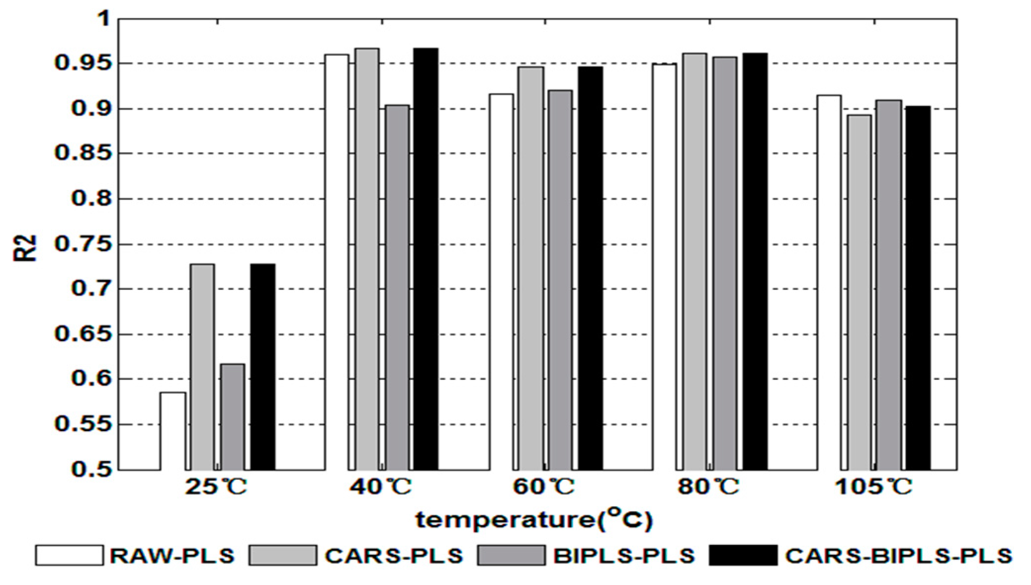
The prediction results with different model methods are shown in Figure 5. From the aspect of detection accuracy, no matter which method was used, the detection accuracy of soil nitrogen was the worst when soil was detected after a 25 °C placement ($0.585<R_p^2<0.728$). Besides this, the detection accuracy achieved was much better ($0.916<R_p^2<0.966$) when the drying temperature ranged from 40 °C to 80 °C. Meanwhile, when the drying temperature rose to 105 °C, the $R_p^2$ of soil nitrogen detection dropped to about 0.9. It was indicated that drying temperature did affect the calcium soil nitrogen detection, and that a low or extremely high drying temperature was adverse to soil nitrogen detection. From the aspects of algorithms effects, CARS-BIPLS-PLS achieved the best detection effects compared to other methods. The reason might be that the most useful characteristic variables were selected and combined by CARS and BIPLS. Moreover, the soil nitrogen detection effects of BIPLS-PLS were not stable and worse than those of CARS-BIPLS-PLS and CARS-BPLS when soil was dried at 40 °C and at a 25 °C placement. The reason was that it was difficult to find the best characteristic intervals of the soil spectrum for all drying temperatures, and some effective spectral information might be removed [31]. Also, some noise information was preserved in the original spectra in RAW-PLS, especially when soil was detected after a 25 °C placement, which was caused by the preserved water content in the soil.

4. Conclusions

In order to investigate the effects of drying temperature on calcium soil nitrogen detection and its characteristic bands by NIR spectroscopy, calcium soil was detected using NIR spectroscopy after five different temperatures. The spectra were pretreated by five preprocessing methods, the characteristic bands and intervals were selected by CARS and BIPLS, and PLS was used to model and analyze the spectral data.

The main conclusions are as follows: (1) The drying temperature did have an obvious influence on soil nitrogen detection using NIR spectroscopy, and it was necessary to find the suitable drying temperature and spectral pretreatments to enhance the detection accuracy; (2) the drying temperatures ranging from 40 °C to 80 °C of calcium soil nitrogen detection accuracy were the best. The calcium soil nitrogen detection had the worst results when soil was placed at 25 °C. The O–H bond in soil might be the main factor that influenced the prediction accuracy; (3) the prediction effect of soil nitrogen was at its optimum using the method of CARS-BIPLS-PLS. In general, the drying temperature had an obvious influence on the detection of soil nitrogen by NIR, and the suitable drying temperature was of great significance to enhance the detection accuracy.

References

- Todorova, M.; Atanassova, S.; Lange, H.; Pavlov, D. Estimation of total N, total P, pH and electrical conductivity in soil by near-infrared reflectance spectroscopy. Agric. Sci. Technol. 2011, 3, 50–54. [Google Scholar]
- Muñozhuerta, R.F.; Guevaragonzalez, R.G.; Contrerasmedina, L.M.; Torrespacheco, I.; Pradoolivarez, J.; Ocampovelazquez, R.V. A Review of Methods for Sensing the Nitrogen Status in Plants: Advantages, Disadvantages and Recent Advances. Sensors 2013, 13, 10823–10843. [Google Scholar] [CrossRef] [PubMed]
- Suehara, K.I.; Nakano, Y.; Yano, T. Simultaneous measurement of carbon and nitrogen content of compost using NIR spectroscopy. J. Near Infrared Spectrosc. 2001, 9, 35–41. [Google Scholar] [CrossRef]
- Ben-dor, E.; Banin, A. Near-infrared analysis as a rapid method to simultaneously evaluate several soil properties. Soil Sci. Soc. Am. J. 1995, 59, 364–372. [Google Scholar] [CrossRef]
- Zornoza, R.; Guerrero, C.; Mataix-Solera, J.; Scow, K.M.; Arcenegui, V.; Mataix-Beneyto, J. Near infrared spectroscopy for determination of various physical, chemical and biochemical properties in Mediterranean soils. Soil Biol. Biochem. 2008, 40, 1923–1930. [Google Scholar] [CrossRef] [PubMed]
- Dalal, R.C. Simultaneous determination of moisture, organic carbon, and total nitrogen by near infrared reflectance spectrophotometry. Soil Sci. Soc. Am. J. 1986, 50, 120–123. [Google Scholar] [CrossRef]
- He, Y.; Huang, M.; García, A.; Hernández, A.; Song, H. Prediction of soil macronutrients content using near-infrared sensors. Comput. Electron. Agric. 2007, 58, 144–153. [Google Scholar] [CrossRef]
- Barthès, B.; Brunet, D.; Ferrer, H.; Chotte, J.L.; Feller, C. Determination of total carbon and nitrogen content in a range of tropical soils using near infrared spectroscopy: Influence of replication and sample grinding and drying. J. Near Infrared Spectrosc. 2006, 14, 341–348. [Google Scholar] [CrossRef]
- Zhang, Y.; Li, M.Z.; Zheng, L.H.; Zhao, Y.; Pei, X. Soil nitrogen content forecasting based on real-time NIR spectroscopy. Comput. Electron. Agric. 2016, 124, 29–36. [Google Scholar] [CrossRef]
- Lu, Y.; Bai, Y.; Lei, W.; He, W.; Yang, L. Determination for total nitrogen content in black soil using hyperspectral data. Trans. Chin. Soc. Agric. Eng. 2010, 26, 256–261. [Google Scholar]
- Shi, T.; Cui, L.; Wang, J.; Fei, T.; Chen, Y.; Wu, G. Comparison of multivariate methods for estimating soil total nitrogen with visible/near-infrared spectroscopy. Plant Soil 2013, 366, 363–375. [Google Scholar] [CrossRef]
- He, Y.; Hu, K.L.; Li, B.; Chen, D.; Suter, H.; Huang, Y. Comparison of sequential indicator simulation and transition probability indicator simulation used to model clay content in microscale surface soil. Soil Sci. 2009, 174, 395–402. [Google Scholar] [CrossRef]
- Reeves, J.B.; McCarty, G.W.; Reeves, V.B. Mid-infrared Diffuse Reflectance Spectroscopy for the Quantitative Analysis of Agricultural Soils. J. Agric. Food Chem. 2001, 49, 766–772. [Google Scholar] [CrossRef] [PubMed]
- Chen, S.; Edwards, C.A.; Subler, S. The influence of two agricultural biostimulants on nitrogen transformations, microbial activity, and plant growth in soil microcosms. Soil Biol. Biochem. 2003, 35, 9–19. [Google Scholar] [CrossRef]
- Cartes, P.; Jara, A.A.; Demanet, R.; Mora, M.D.L.L. Urease activity and nitrogen mineralization kinetics as affected by temperature and urea input rate in southern chilean andisols. J. Soil Sci. Plant Nutr. 2009, 9, 69–82. [Google Scholar] [CrossRef]
- Fystro, G. The prediction of C and N content and their potential mineralisation in heterogeneous soil samples using Vis-NIR spectroscopy and comparative methods. Plant Soil 2002, 246, 139–149. [Google Scholar] [CrossRef]
- Bo, S. Effects of soil sample pretreatments and standardised rewetting as interacted with sand classes on Vis-NIR predictions of clay and soil organic carbon. Geoderma 2010, 158, 15–22. [Google Scholar]
- Mouazen, A.M.; Baerdemaeker, J.D.; Ramon, H. Towards development of on-line soil moisture content sensor using a fibre-type nir spectrophotometer. Soil Tillage Res. 2005, 80, 171–183. [Google Scholar] [CrossRef]
- Nie, P.C.; Dong, T.; He, Y.; Qu, F.F. Detection of soil nitrogen using near infrared sensors based on soil pretreatment and algorithms. Sensors 2017, 17, 1102. [Google Scholar] [CrossRef] [PubMed]
- He, Y.; Xiao, S.; Nie, P.; Dong, T.; Qu, F.; Lin, L. Research on the optimum water content of detecting soil nitrogen using near infrared sensor. Sensors 2017, 17, 2045. [Google Scholar] [CrossRef] [PubMed]
- Kuang, B.; Mouazen, A.M. Non-biased prediction of soil organic carbon and inorganic nitrogen with vis–NIR spectroscopy, as affected by soil moisture content and texture. Biosyst. Eng. 2013, 114, 249–258. [Google Scholar] [CrossRef] [Green Version]
- Nduwamungu, C.; Ziadi, N.; Tremblay, G.F.; Parent, L.É. Near-infrared reflectance spectroscopy prediction of soil properties: Effects of sample cups and preparation. Soil Sci. Soc. Am. J. 2009, 73, 1896–1903. [Google Scholar] [CrossRef]
- Tian, Y.; Zhang, J.; Yao, X.; Cao, W.; Zhu, Y. Laboratory assessment of three quantitative methods for estimating the organic matter content of soils in china based on visible/near-infrared reflectance spectra. Geoderma 2013, 202, 161–170. [Google Scholar] [CrossRef]
- Brunet, D.; Barthès, B.G.; Chotte, J.L.; Feller, C. Determination of carbon and nitrogen contents in alfisols, oxisols and ultisols from africa and brazil using nirs analysis: Effects of sample grinding and set heterogeneity. Geoderma 2007, 139, 106–117. [Google Scholar] [CrossRef]
- Gorry, P.A. General least-squares smoothing and differentiation by the convolution (Savitzky-Golay) method. Anal. Chem. 1990, 62, 570–573. [Google Scholar] [CrossRef]
- Chen, J.; Jönsson, P.; Tamura, M.; Gu, Z.; Matsushita, B.; Eklundh, L. A simple method for reconstructing a high-quality NDVI time-series data set based on the Savitzky–Golay filter. Remote Sens. Environ. 2004, 91, 332–344. [Google Scholar] [CrossRef]
- Isaksson, T.; Næs, T. The Effect of Multiplicative Scatter Correction (MSC) and Linearity Improvement in NIR Spectroscopy. Appl. Spectrosc. 1988, 42, 1273–1284. [Google Scholar] [CrossRef]
- Hsu, H.; Binder, K.; Paul, W. How to define variation of physical properties normal to an undulating one-dimensional object. Phys. Rev. Lett. 2009, 103, 198301. [Google Scholar] [CrossRef] [PubMed]
- Wen, L.; Bai, Z.; Bai, J.; Guo, Z. Decomposition kinetics of hydrogen bonds in coal by a new method of in-situ diffuse reflectance ft-ir. J. Fuel Chem. Technol. 2011, 39, 321–327. [Google Scholar]
- Parvinnia, E.; Sabeti, M.; Jahromi, M.Z.; Boostani, R. Classification of eeg signals using adaptive weighted distance nearest neighbor algorithm. J. King Saud Univ. Comput. Inf. Sci. 2014, 26, 1–6. [Google Scholar] [CrossRef]
- Li, X.; He, Y.; Wu, C.; Sun, D. Nondestructive measurement and fingerprint analysis of soluble solid content of tea soft drink based on vis/nir spectroscopy. J. Food Eng. 2007, 82, 316–323. [Google Scholar] [CrossRef]
- Yang, M.H.; Zhao, X.M. Study on soil total n estimation by vis-nir spectra with variable selection. Sci. Agric. Sinica 2014, 47, 2374–2383. [Google Scholar]
- Cramer, J.A.; Kramer, K.E.; Johnson, K.J.; Morris, R.E.; Rose-Pehrsson, S.L. Automated wavelength selection for spectroscopic fuel models by symmetrically contracting repeated unmoving window partial least squares. Chemom. Intell. Lab. Syst. 2008, 92, 13–21. [Google Scholar] [CrossRef]
- Lindberg, W.; Persson, J.A.; Wold, S. Partial least-squares method for spectrofluorimetric analysis of mixtures of humic acid and lignin sulfonate. Anal. Chem. 1983, 55, 643–648. [Google Scholar] [CrossRef]
- Trygg, J.; Wold, S. Pls regression on wavelet compressed nir spectra. Chemom. Intell. Lab. Syst. 1998, 42, 209–220. [Google Scholar] [CrossRef]
- Kawamura, K.; Tsujimoto, Y.; Rabenarivo, M.; Asai, H.; Andriamananjara, A.; Rakotoson, T. Vis-NIR Spectroscopy and PLS Regression with Waveband Selection for Estimating the Total C and N of Paddy Soils in Madagascar. Remote Sens. 2017, 9, 1081. [Google Scholar] [CrossRef]
- Fuwa, K.; Valle, B.L. The physical basis of analytical atomic absorption spectrometry. The pertinence of the beer-lambert law. Anal. Chem. 1963, 35, 942–946. [Google Scholar] [CrossRef]
- Libowitzky, E. Correlation of O-H stretching frequencies and O-H…O hydrogen bond lengths in minerals Korrelation von O-H-Streckfrequenzen und O-R…O-Wasserstoffbrückenlängen in Mineralen. Monatshefte Für Chem. 1999, 130, 1047–1059. [Google Scholar]
- Zhan, X.; Zhao, N.; Lin, Z.; Wu, Z.; Yuan, R.; Qiao, Y. Effect of algorithms for calibration set selection on quantitatively determining asiaticoside content in centella total glucosides by NIR spectroscopy. Spectrosc. Spectr. Anal. 2014, 34, 3267–3272. [Google Scholar]
- Alahmadi, Y.J.; Gholami, A.; Fridgen, T.D. The protonated and sodiated dimers of proline studied by IRMPD spectroscopy in the N-H and O-H stretching region and computational methods. Phys. Chem. Chem. Phys. 2014, 16, 26855–26863. [Google Scholar] [CrossRef] [PubMed]
Figure 1.
Soil average spectra with different spectra pretreated after drying at 40 °C. (a) The raw spectra; (b) the spectra after Savitzky–Golay (S–G) smoothing pretreatment; (c) the spectra after multiplicative scatter correction (MSC) processing; (d) the spectra with standard normal variation (SNV) pretreatment; (e) the detrending (DT)-treated spectra; (f) the spectra after 1st-Derivation (1st-Der).
Figure 2.
The average spectral of different drying temperatures when the soil nitrogen concentration is 2.5 g/kg.
Figure 3.
(a) The determination coefficients of the partial least squares (PLS) method after different spectral pretreatments; (b) the prediction results of the RAW-PLS model at different temperatures.
Figure 4.
The sensitive waveband selection process: (a) The characteristic variables selected by competitive adaptive reweighted squares (CARS); (b) the number of PLS components and the corresponding the root mean square error of cross validation (RMSECV) values while running Backward Interval Partial Least Squares (BIPLS); (c) the characteristic intervals determined by BIPLS.
Figure 5.
The comparison of different algorithms.