Prioritization Assessment for Capability Gaps in Weapon System of Systems Based on the Conditional Evidential Network


1
Aerospace Command Academy, Space Engineering University, Beijing 101416, China
2
Science and Technology on Complex Electronic System Simulation Laboratory, Space Engineering University, Beijing 101416, China
3
Complex System Simulation Lab, Beijing Institute of System Engineering, Beijing 100101, China
*
Author to whom correspondence should be addressed.
Appl. Sci. 2018, 8(2), 265; https://doi.org/10.3390/app8020265
Submission received: 18 January 2018
/
Revised: 18 January 2018
/
Accepted: 6 February 2018
/
Published: 11 February 2018
Abstract
:The prioritization of capability gaps for weapon system of systems is the basis for design and capability planning in the system of systems development process. In order to address input information uncertainties, the prioritization of capability gaps is computed in two steps using the conditional evidential network method. First, we evaluated the belief distribution of degree of required satisfaction for capabilities, and then calculated the reverse conditional belief function between capability hierarchies. We also provided verification for the feasibility and effectiveness of the proposed method through a prioritization of capability gaps calculation using an example of a spatial-navigation-and-positioning system of systems.
1. Introduction
A capability gap is defined by the degree to which a designated action plan of the system of systems cannot be implemented. Such a gap may result from a lack of capability, proficiency in existing capability solutions, and/or the need to replace existing capability solutions to prevent future gaps.
Operational requirements often require more capabilities than equipment developments are able to provide. A capability gap describes the difference between the status of the system of systems’ capabilities and the operational requirements. It is a direct base for maximum capability realization of the system of systems. The purpose of a gap assessment is to identify its size and determine the weaknesses of supported equipment demonstration.
Capability-gap analysis mainly includes two aspects. The first, in response to the functional needs of the capability, is to carry out an assessment of the capabilities in the weapon system of systems. The second aspect consists in comparing the status of the capability needs and the capabilities one by one, according to criteria, such as “be able to support well”, “be able to support under certain conditions”, and “cannot support”, as well as analyzing whether these capabilities support the completion of the task.
1.1. Evidential Network
Knowledge representation and uncertainty reasoning based on the network-based method began with research on early constrained networks, qualitative Markov trees [1], and qualitative Markov networks [2]. In the late 1980s and early 1990s, the Bayesian Network (BN) [3] and the value-based system (VBS) [4] greatly promoted the use of a network model for knowledge representation and uncertainty inference. However, BN and VBS cannot handle knowledge that is described as a belief function. Cano put forward an axiomatic reasoning system in 1993 [5] that extracts an abstract mathematical model so as to represent information by expressing concepts and algorithms that are related to the value, and that provide a general framework for studying knowledge representation and reasoning in causal networks, including probability and belief functions. General information can then be decomposed from a generalized conditional-probability perspective. That same year, Smets, the author of the transitive belief model (TBM), proposed a generalized Bayesian theory (GBT) [6] under the framework of the TBM. By means of the Disjunctive Rule of Combination (DRC), where only one of the two independent evidences is known, the belief of both evidences can be calculated, which is to say that the belief function also has the same conditional belief function as the Bayesian formula. Based on these two basic theoretical achievements, some scholars began to explore the modeling and reasoning of evidence networks. In 1994, Xu and Smets first proposed the concept of evidential networks (EN) [7] and for the first time used the conditional belief function to represent the relationship between network nodes. This paper proposes the concept of using the evidential network with a conditional belief function (ENC) and offers the corresponding reasoning algorithm. By analyzing the characteristics of ENC, this paper also explores reasoning that may simplify the problem.
Attoh-Okine and Bovee et al. proposed an understanding of the evidential network based on the qualitative Markov tree [8,9]. Cobb and Yaghlane et al. by comparing and analyzing the similarities and differences between the evidence network and the VBS, pointed out that the main problem of evidential-network research is how to represent the independence of the belief function through the graph model. Based on the general belief function and the transitive belief function, a model of the directed belief network with the conditional belief function (DEVN) was proposed. The relationship between knowledge and conditions in the network was represented by a directed acyclic graph plus the belief function, and the EN reasoning was realized through DRC and GBT [10,11,12]. Srivastava et al. obtained the causal graph through an explicit causal matching algorithm and then constructed the evidential network by using the basic concepts of the belief function. Expansion and marginalization were used in the reasoning process to solve the problem of job-satisfaction evaluation [13]. Simon and Weber published five consecutive articles from 2007–2009, combining Bayesian networks and evidence theory in order to solve the reliability problems in complex systems, which mainly involve incomplete and inaccurate information. Their reasoning mode is still used in Bayesian theory [14,15,16,17,18]. Trained as a Yaghlane student, Trabelsi developed a BeliefNet tool in 2008 that combines the synthesis, marginalization, expansion, and projection algorithms of the evidential network with inference algorithms such as binary syndication and hash tables [19].
In 2012, Wafa and Yaghlane used a dynamically-directed evidential network with conditional belief functions for a study on system reliability, indicating that the directed evidential network is moving toward a dynamic direction [20]. Later, in 2013, they proposed a new propagation algorithm for a dynamic directed evidence network with conditional belief functions, based on a new computational structure called Mixed Binary Tree [21]. This algorithm is suitable for accurate reasoning. In 2014, Wafa published two consecutive articles, in which Monte Carlo algorithms were used to discuss both the reasoning of single-connected directed evidential networks with conditional belief functions and the approximate reasoning of directed evidential networks with conditional belief functions [22,23]. In terms of evidential-network learning, Hariz and Yaghlane published two articles in 2014 on the parametric learning of conditional-belief evidential networks [24,25], and in an article published in 2015 used an evidence database to discuss the structural learning of evidential networks [26]. In 2015, Wafa and Yaghlane explored the propagation of belief functions in single-connected hybrid directed evidential networks [27]. A hybrid directed evidential network is a promotion of a standard directed evidential network, bringing the development of evidential network one step further.
1.2. Prioritization Assessment of Capability Gaps
There is little research in China that focuses on the priority assessment of capability gaps. Some research in this field exists abroad, but most of it is qualitative. The Technical Cooperation Program (TTCP) joint system and analysis team presents a qualitative analysis method that uses colors to identify the importance of capability gaps [36]. This is a completely subjective and sketchy approach. The US military “Capabilities-Based Assessment Handbook 3.0” introduced the sequencing of biometric information recognition-related capability gaps [37]. This method is based on a comparison of capability gaps among experts, regardless of uncertainty. Linkov, from the research and development center at the US Army Corps of Engineers, examined the issue of capability gaps in the small-arms program for multi-service, using a multi-criteria decision analysis method [38]. The core of this method is an analytic hierarchy process, but its disadvantage is that there is no verification of the consistency of the judgment matrix. Hristov proposed a prioritization method for capability gaps, which was used to solve the problem of how to rank gaps in the combat capability of the Bulgarian armed forces [39]. This method takes into account three factors: the weight of the capability, the expected utility after filling the capability gap, and its urgency. It does not, however, consider the uncertainty. Welch proposed a gap-ranking method based on the utility theory, which is used to solve the capability-gap ranking problem of brigade combat units [40]. This method is part of the United States-based Sandia National Laboratory Modernization assessment process. Most of the work needs to be completed by experts in relevant fields, and the method is subjective.
Langford rethinks the theoretical basis and systematic study of gap analysis, and expands on it while delineating its practicality and limitation. He came up with new ideas on these theoretical foundations by adopting the perspective of systems and value engineering [41]. By qualitatively analyzing the gap in the medium-lift capability of the United States Marine Corps, Harris suggested that a medium-lift platform be added to fill the capability gap between light- and heavy-duty lift planes [42]. By analyzing the capabilities gap, John of the United States Army argued that the quest for high-end capabilities left the Australian Defense Force vulnerable to mission failures, following which he finally obtained the prioritization of defense major capabilities [43]. By combining the soldier’s expertise with a quantifiable analysis, Rubemeyer proposed a gap-assessment method [44]. In this method, combatants on the mission determine the impact of measurable attributes from each capability gap; a mathematical approach is used to incorporate all of the combatants’ responses into a single mission impact for each capability gap. In order to identify Air Force characteristics, the Office of Aerospace Studies of the United States Air Force conducts research on the methods and processes of capability-gap analysis through capability requirement statements, capability gap identification, capability gap statements, gap characterization, risk assessment, and gap prioritization [45]. In order for the Department of Homeland Security’s capability to deal with biochemical threats, the U.S. Government Accountability Office submitted a report to the National Congress that elaborated the need for an analysis of the relevant capability gaps and put forward ways to identify and resolve related capability gaps [46]. These methods are qualitative and do not account for uncertainty.
In this paper, in which we focused on the multiple uncertainties in the priority assessment of capability gaps, we adopted a method based on the conditional evidential network. Using the space-navigation-and-positioning system of systems as an example, we studied the priority assessment of capability gaps in weapon system of systems.
2. Basics of the Conditional Evidential Network
In belief function theory, is a set of mutually exclusive and complete finite elements, called the recognition framework. is its power set.
The belief distribution that supports proposition A is called the basic belief assignment (BBA) and is a function that maps from to [0, 1], as shown in the following equation:
If any subset basic belief assignment , then A is called a focal element of Θ.
Each basic belief assignment m is associated with a belief function Bel mapped from to [0, 1] and a likelihood function Pl mapped from to [0, 1]. These two functions represent the smallest and largest possible support for A, respectively. These functions are defined as follows:
A belief function is a Bayesian function if and only if there is a unique function such that for , holds, and holds.
Compared with the Bayesian function, the belief function is a set functions, and the Bayesian function is a point function. The Bayesian function is a special case of the belief function, and the belief function is a generalized Bayesian function.
Conditional basic belief , conditional belief function , and conditional likelihood function are defined on the identification framework [47].
Generalized Bayesian Theorem (GBT): Let and be the identification frameworks of X and Y, respectively. Assuming that the identification framework is normalized, that is:
For , the following holds:
When y is one dimension, the following holds:
The conditional belief function and conditional likelihood function still hold the following relations:
Therefore:
The following holds:
Forward reasoning: If we know the belief information on each state or subset of Y, denoted as , , then for , the following holds:
The above formula is based on the conditional basic belief. By the same token, the above equation, expressed with the conditional belief function and conditional likelihood function, reads:
Marginalization: Let the conditional belief function be the marginal conditional belief function of on X and be the marginal conditional likelihood function of on X. The following holds:
3. Capability Gaps Computing Based on the Conditional Evidential Network
This paper specifically sorts the capability-gap priorities of weapon system of systems based on the power product of the inverse conditional belief functions and . means that the upper-level capability’s requirement satisfaction is low, while means that the lower-level capability’s requirement-satisfaction is low. represents the belief distribution of the degree of requirement satisfaction of the lower-level capability. represents the belief distribution of the degree of requirement satisfaction of the lower-level capability when that of the upper-level capability is low. reflects the gap in capability in an intuitive manner, while reflects the degree of influence of the given gap on the upper-level capability gap. The power product of the two can help with a more comprehensive assessment of capability-gap priorities.
3.1. Calculation of the Belief Distribution of the Requirement-Satisfaction Degree for Capabilities
To calculate the belief distribution of the requirement-satisfaction degree for capabilities, first we need to establish the conditional-evidential-network identification framework and the conditional-belief-parameter table.
We use a causality diagram along with other methods in order to construct the evidential network of weapon system of systems’ capabilities. In order to model it, we use the conditional belief function, based on relevant knowledge and experts’ experience. Following this, we obtain the evidential-network structure-chart and conditional-belief-function table. The conditional belief function in this paper is defined by each node and expressed in , where C represents the state of the capability sub-node and represents the combined state of all of the node’s parent nodes.
Next, we calculate the belief distribution of the requirement-satisfaction degree of the bottom capability.
Let and respectively denote the ideal value and the lowest capability-requirement value. c represents the actual value of the capability, represents the credibility of this actual value, and represents the degree to which the actual and ideal values match.
According to the characteristics of the bottom capabilities, the matching degree between the actual and the ideal capabilities can each be calculated according to the indicators of benefit and cost.
- (1)
- The matching degree of the benefit index and the requirement’s ideal value is:
- (2)
- The matching degree of the cost index and the requirement’s ideal value is:
According to the matching degree of the bottom index and the ideal value of the demand, the belief distribution of the requirement satisfaction can be calculated as follows:
where represents the belief that the degree of requirement satisfaction of the bottom indicators is high, represents the belief that it is low, and represents the belief assigned to cognitive uncertainty.
Then we calculate the belief distribution of the requirement-satisfaction degree for the upper layer capability.
According to the conditional-belief-parameter table established using the method in Section 3.1 and the belief distribution of the bottom capability’s requirement satisfaction, the belief distribution of the capability requirement satisfaction for each capability is calculated by the forward reasoning formula:
3.2. Calculation of the Inverse Conditional Belief
The inverse conditional likelihood belief is calculated via the GBT theorem using Equations (9) and (10). The obtained reverse conditional likelihood belief has the joint form for the lower multiple capabilities and must be marginalized. Marginalization is performed according to Equation (14).
The marginalized inverse likelihood function for the lower-level single capabilities can be used directly in Equation (13) to calculate the basic belief function for each capability.
3.3. Prioritization of System of Systems’ Capability Gaps
Based on the product of the belief distribution of the requirement-satisfaction degree for each capability and the reversal basic belief function of each capability obtained through the above steps, the system of systems’ capabilities are prioritized:
where denotes the priority of the lower-level capability gaps, denotes the belief that the requirement-satisfaction degree of the lower-level capability is low, and represents the belief that the degree of requirement satisfaction of the lower-level capability is low under the condition that that of the upper-level capability is low. and .
4. Case Study
This paper applies the above method to assess the prioritization of capability gaps in the space-navigation-and-positioning system of systems, and to verify the above method’s feasibility and effectiveness.
4.1. Construction of the Evidential-Network-Structure Model
Space-navigation-and-positioning system of systems capabilities include navigation and positioning capability, system survivability, system anti-jamming capability, and security and confidentiality. The corresponding evidence network structure was established using the causality-diagram method, as shown in Figure 1.
4.2. The Construction of the Evidential-Network-Parameter Model
The establishment of the recognition framework, corresponding to the evidence network for the capabilities of the space-navigation-and-positioning system of systems in Figure 1, is shown in Table 1. Among the recognition frames, “high” means that the current capability’s situation is “able to support” the capability requirement or that the capability’s degree of requirement satisfaction is high; “medium” means that the capability’s current situation “can support under certain conditions” the capability requirement or that the capability’s degree of requirement satisfaction is normal; and “low” means that the capability status “cannot support” the capability requirement or that the capability’s degree of requirement satisfaction is low. For convenience’s sake, this article divides the top level into three levels and the remaining levels into two.
We took into consideration the fact that satellite navigation signals are likely to be more compressed in actual combat operations and that satellite survivability is more important than ground-station survivability due to the high launch cost of satellites. Encryption capability is more important than anti-virus capability, and navigation-positioning capability is the core competence in spatial-information-support system of systems. The conditional belief functions are calculated by using the weight coefficient of capabilities [48]. Then, we established the belief-parameter table, shown in Figure 2.
In this figure, “m(AJ=H|AC=H, AS=L) = 0.7” indicates that, with the conditional belief of 0.7, the anti-jamming capability of the space-navigation-and-positioning system is “high” when the anti-suppress interference capability is “high” and the anti-spoofing interference capability is “low”. The notation “m(ΘAJ|AC=H, AS=L) = 0.2” indicates that there is a cognitive uncertainty, that is, a partial ignorance of the subject. At this point, we assigned a portion of the belief to the complete set of recognition frames Θ for node states.
4.3. Capability-Requirement-Satisfaction Assessment
Table 2 shows the capability structure parameters of a satellite-navigation-and-positioning system of systems, including sub-capability names, bottom indicators, weights, capability requirements, actual levels, and the credibility of the actual levels.
For example, a positioning accuracy with a confidence level of 0.95 means that the horizontal positioning accuracy is less than or equal to 10 m at a confidence level of 0.95.
Table 3 shows the prior belief distribution of the requirement-satisfaction degree for each index.
We calculated the belief distribution of the requirement-satisfaction degrees of second-layer capabilities using the method described in Section 3.3.
Table 4 and Figure 3 show the belief distributions of the requirement-satisfaction degrees for second-layer capabilities.
Figure 3 shows that the system anti-jamming capability has the highest requirement-satisfaction degree, followed by both system survivability and the navigation-and-positioning capability; the security and confidentiality capability has the lowest requirement-satisfaction degree. In addition, the cognitive uncertainty of the anti-jamming capability is the lowest, and the cognitive uncertainty of the other three capabilities is similar.
4.4. Comparison with the Bayesian Network Method
In order to make a comparison, we created a model using the Bayesian network-based method: we used the same structural model and identification framework employed for the evidential network to establish the conditional-probability-parameter table for capabilities in the space-navigation-and-positioning system of systems.
Figure 4 shows the conditional-probability table for capability indicators defined in the capability-requirement-satisfaction model of the Bayesian network-based space-navigation-and-positioning system of systems.
The difference between Figure 2 and Figure 4 is that, in the event of cognitive uncertainty, the Bayesian network divides cognitive uncertainty into definite states. This is because Bayesian networks cannot handle cognitive uncertainties, so accurate probabilistic judgments are required before reasoning. This will inevitably lead to the loss of uncertain information.
Similarly, the determination of the prior probability of the underlying ability index also requires an accurate probability judgment. Cognitive uncertainty, should it occur, must be assigned to the definite states, as shown in Table 5.
We used the Matlab BNT 1.0.7 toolbox in order to establish, via Figure 1, the structure of the Bayesian network. We then entered the conditional probability distribution (CPD) parameters and the prior probability of the underlying capability index, and obtained the marginal probability of each capability, as shown in Table 6.
We compared Table 4 and Table 6 to the data shown in Figure 5. We obtained AJ, SS, SC, NP through the evidence-based method and AJ’, SS’, SC’, NP’ through the Bayesian-based method. The requirement-satisfaction degree with the highest value corresponds to the anti-jamming capability in the results obtained via the evidential network, while it corresponds to system survivability for results obtained through the Bayesian network.
The methods—Bayesian and evidential—used to assess the degree of capability requirement satisfaction differed in mainly two aspects: parameter modeling and reasoning methods.
The difference between parameter modeling in Bayesian networks and evidential networks is that the former requires an accurate probability judgment, while the latter does not. Moreover, the latter can both model cognitive uncertainty and handle the aspects that involve the researcher’s ignorance on the subject.
The difference between reasoning methods in Bayesian and evidential networks is that the former must make a fuzzy estimation of prior knowledge before initiating the reasoning process. However, fuzzy estimations often yield invalid results that can be used for reasoning when the individual state probabilities of the variables are similar. Even if the results are valid, some uncertain information will be lost. The reasoning method based on evidential networks does not need a fuzzy estimation of the evidence of uncertainty, thus avoiding the loss of uncertain information to an optimal degree. It is able to obtain more accurate results while avoiding misjudgment.
In addition, evidential network-based reasoning methods can combine multiple uncertain evidences that are passed to a node directly through Dempster’s combination rules. A combined evidence of information is then formed and transferred to the adjacent node. This avoids double-counting multiple pieces of evidence in the same path; it can be said that this model is an efficient parallel-computing model. In the Bayesian network, the reasoning method’s mechanism-of-combination rule is unable to fuse uncertain evidences due to the fact that the use of probability is the basis of the uncertainty reasoning: every piece of evidence information is required to travel through the entire network. After updating all of the nodes’ probability values as one new prior probability, the same operations can be performed on other nodes’ evidences in order to update the multi-evidence information. For the complex network, the computational complexity of the Bayesian network makes it difficult to complete the reasoning task. Conversely, the evidential network-based reasoning method greatly improves and accelerates the efficiency of the reasoning.
4.5. Calculation of the Inverse Conditional Belief Functions
Following the method described in Section 3.2, GBT was used to calculate the inverse conditional belief. We first calculated the inverse conditional likelihood function. After marginalization, we obtained the inverse conditional basic belief function. The reverse conditional likelihood function calculation process is as follows:
Similarly, we can obtain other reverse conditional likelihood functions, as shown in Table 7.
For which:
The calculation of the inverse conditional basic belief function after marginalization is as follows:
Similarly, we can obtain other reverse conditional basic belief functions as follows:
4.6. Prioritization of Capability Gaps
Finally, we calculated the priority of capability gaps in layer 2, as described in Section 3.3., where and are both 0.5.
The priority of system of systems’ capability gaps was calculated as follows:
The priority ranking result of capability gaps is as follows:
AJ >> SC >> SS >>NP
4.7. Results and Analysis
Figure 6 shows that the system’s anti-jamming capability gap has the highest priority, followed by both the security-and-confidentiality capability and the system survivability, with the navigation-and-positioning capability gap having the lowest priority. In order to improve the degree of requirement satisfaction in the entire space-navigation-and-positioning system of systems, measures must focus on improving the system’s anti-jamming capability.
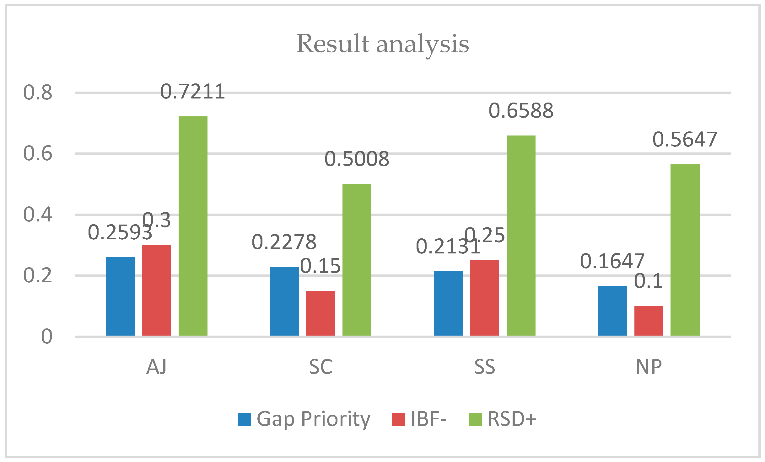
In Figure 7, “Gap Priority” indicates the capability-gap priority, “IBF−” indicates the inverse belief function value, and “RSD+” indicates the belief with a high degree of requirement satisfaction, calculated using the method in Section 3.1.
While, as shown in Figure 6, the degree of requirement satisfaction of the anti-jamming capability has the highest value, it also remains the top final gap priority as it has the largest inverse-belief-function value.
We used a conditional evidential network in order to assess the prioritization of capability gaps in space-navigation-and-positioning system of systems. This network is able to efficiently handle the experience of relevant experts while making full use of the input of uncertain knowledge. This all helps to improve the credibility of capability assessment in space-navigation-and-positioning system of systems.
5. Conclusions
The assessment of capability-gap priority in weapon system of systems is the basis for equipment and non-equipment solutions for solving capability gaps. Based on the conditional evidential network, this paper evaluates the priority of capability gaps for weapon system of systems from a purely quantitative perspective. Compared with qualitative methods, this method enhances the credibility of the assessment work. In addition, this method integrates many different forms of input data and various uncertain information into a unified belief expression framework, thus facilitating the assessment of a large-scale weapon system of systems. Unlike the Bayesian network-based approach, the evidential network-based approach does not require accurate probabilistic judgments and fuzzy estimates, minimizing the loss of uncertain information. In addition, it can handle cognitive uncertainty. It is therefore able to obtain results in evidence reasoning that are more accurate, while avoiding misjudgment. Having conducted a case analysis, we consider this method to be both feasible and effective.
Acknowledgments
The authors are grateful to the National 863 Fund Project (No. 2014AA7013034) and the National Defense Pre-Research Fund Project (No. 414050201) for their financial support.
Author Contributions
Dong Pei and Daguo Qin conceived and designed the evidential network model; Dong Pei studied the case, Yang Sun, Guangzhi Bu, and Zhonghua Yao helped in the case study; Dong Pei analyzed the data; Dong Pei wrote the paper.
Conflicts of Interest
The authors declare no conflict of interest.
References
- Shafer, G.; Shenoy, P.P.; Mellouli, K. Propagating belief functions in qualitative Markov trees. Int. J. Approx. Reason. 1987, 1, 349–400. [Google Scholar] [CrossRef]
- Mellouli, K.; Shafer, G.; Shenoy, P.P. Qualitative Markov Networks. In Proceedings of the 1986 International Conference on Information Processing and Management of Uncertainty in Knowledge-Based Systems (IPMU 1986), Paris, France, 30 June–4 July 1986. [Google Scholar]
- Pearl, J. Probabilistic Reasoning in Intelligent Systems: Network of Plausible Inference; Morgan Kaufmann, Inc.: San Mateo, CA, USA, 1988. [Google Scholar]
- Shenoy, P.P. Valuation-Based Systems: A framework for managing uncertainty in expert systems. In Fuzzy Logic for the Management of Uncertainty; Zadeh, L.A., Kacprzyk, J., Eds.; John Wiley & Sons: New York, NY, USA, 1992; pp. 83–104. [Google Scholar]
- Cano, J.; Delgado, M.; Moral, S. An axiomatic framework for propagation uncertainty in directed acyclic networks. Int. J. Approx. Reason. 1993, 8, 253–280. [Google Scholar] [CrossRef]
- Smets, P. Belief fucntions: The disjunctive rule of combination and the generalized bayesian theorem. Int. J. Approx. Reason. 1993, 9, 1–35. [Google Scholar] [CrossRef]
- Xu, H.; Smets, P. Reasoning in evidential networks with conditional belief functions. Int. J. Approx. Reason. 1996, 14, 155–185. [Google Scholar] [CrossRef]
- Attoh-Okine, N.O. Aggregating evidence in pavement management decision-making using belief functions and qualitative Markov tree. IEEE Trans. Syst. Man Cybern. 2002, 32, 243–251. [Google Scholar] [CrossRef]
- Bovee, M.; Srivastava, R.P.; Mak, B. A conceptual framework and belief-function approach to assessing overall information quality. Int. J. Intell. Syst. 2003, 18, 51–74. [Google Scholar] [CrossRef]
- Cobb, B.R.; Shenoy, P.P. A comparison of bayesian and belief function reasoning. Inf. Syst. Front. 2003, 5, 345–358. [Google Scholar] [CrossRef]
- Yaghlane, B.B.; Smets, P.; Mellouli, K. Directed Evidential Networks with Conditional Belief Functions. In Proceedings of the 7th European Conference Symbolic and Quantitative Approaches to Reasoning with Uncertainty (ECSQARU 2003), Aalborg, Denmark, 2–5 July 2003. [Google Scholar]
- Yaghlane, B.B.; Mellouli, K. Inference in directed evidential networks based on the transferable belief model. Int. J. Approx. Reason. 2008, 48, 399–418. [Google Scholar] [CrossRef]
- Srivastava, R.P.; Buche, M.W.; Roberts, T.L. Belief function approach to evidential reasoning in causal maps. In Causal Mapping for Research in Information Technology; Narayanan, V.K., Armstrong, D.J., Eds.; IGI Global: Hershey, PA, USA, 2005; pp. 109–141. [Google Scholar]
- Simon, C.; Weber, P.; Levrat, E. Bayesian networks and evidence theory to model complex systems belief. J. Comput. 2007, 2, 33–43. [Google Scholar] [CrossRef]
- Weber, P.; Simon, C. Dynamic Evidential Networks in System Belief Analysis: A Dempster Shafer Approach. In Proceedings of the 16th Mediterranean Conference on Control and Automation (MED 2008), Ajaccio, France, 25–27 June 2008. [Google Scholar]
- Simon, C.; Weber, P.; Evsukoff, A. Bayesian networks inference algorithm to implement Dempster Shafer theory in belief analysis. Belief Eng. Syst. Saf. 2008, 93, 950–963. [Google Scholar] [CrossRef]
- Simon, C.; Weber, P. Imprecise belief by evidential networks. J. Risk Belief 2009, 223, 119–131. [Google Scholar]
- Simon, C.; Weber, P. Evidential networks for belief analysis and performance evaluation of systems with imprecise knowledge. IEEE Trans. Belief 2009, 58, 69–87. [Google Scholar]
- Trabelsi, W.; Yaghlane, B.B. BeliefNet Tool: An Evidential Network Toolbox for Matlab. In Proceedings of the 2008 International Conference on Information Processing and Management of Uncertainty in Knowledge-Based Systems (IPMU 2008), Malaga, Spain, 22–27 June 2008. [Google Scholar]
- Laamari, W.; Yaghlane, B.B.; Simon, C. Dynamic Directed Evidential Networks with Conditional Belief Functions: Application to System Belief. In Proceedings of the 2012 International Conference on Information Processing and Management of Uncertainty in Knowledge-Based Systems (IPMU 2012), Catania, Italy, 9–13 July 2012. [Google Scholar]
- Laamari, W.; Yaghlane, B.B.; Simon, C. New Propagation Algorithm in Dynamic Directed Evidential Networks with Conditional Belief Functions. In Proceedings of the 2013 International Symposium on Integrated Uncertainty in Knowledge Modelling and Decision Making (IUKM 2013), Beijing, China, 12–14 July 2013. [Google Scholar]
- Laamari, W.; Yaghlane, B.B. Reasoning in Singly-Connected Directed Evidential Networks with Conditional Beliefs. In Proceedings of the 8th Hellenic Conference on AI, SETN 2014, Ioannina, Greece, 15–17 May 2014. [Google Scholar]
- Laamari, W.; Hariz, N.B.; Yaghlane, B.B. Approximate Inference in Directed Evidential Networks with Conditional Belief Functions Using the Monte Carlo Algorithm. In Proceedings of the 15th International Conference on Information Processing and Management of Uncertainty in Knowledge-Based Systems (IPMU 2014), Montpellier, France, 15–19 July 2014. [Google Scholar]
- Hariz, N.B.; Yaghlane, B.B. Learning Parameters in Directed Evidential Networks with Conditional Belief Functions. In Proceedings of the Third International Conference on Belief Functions (BELIEF 2014), Oxford, UK, 26–28 September 2014. [Google Scholar]
- Hariz, N.B.; Yaghlane, B.B. Incremental Method for Learning Parameters in Evidential Networks. In Proceedings of the 30th International Conference on Industrial, Engineering, Other Applications of Applied Intelligent Systems, Arras, France, 27–30 June 2017. [Google Scholar]
- Hariz, N.B.; Yaghlane, B.B. Learning Structure in Evidential Networks from Evidential DataBases. In Proceedings of the 13th European Conference on Symbolic and Quantitative Approaches to Reasoning with Uncertainty (ECSQARU 2015), Compiègne, France, 15–17 July 2015. [Google Scholar]
- Laamari, W.; Yaghlane, B.B. Propagation of Belief Functions in Singly-Connected Hybrid Directed Evidential Networks. In Proceedings of the STANFORD-USTC-MIT 2015 Geoscience Summer Camp, Hefei, China, 6–15 September 2015. [Google Scholar]
- Benavoli, A.; Ristic, B.; Farina, A.; Oxenham, M.; Chisci, L. An application of evidential networks to threat assessment. IEEE Trans. Aerosp. Electron. Syst. 2009, 45, 620–639. [Google Scholar] [CrossRef]
- Hong, X.; Nugent, C.; Mulvenna, M.; Mcclean, S.; Scotney, B.; Devlin, S. Evidential fusion of sensor data for activity recognition in smart homes. Pervasive Mob. Comput. 2009, 5, 236–252. [Google Scholar] [CrossRef]
- Lee, H.; Choi, J.S.; Elmasri, R. A static evidential network for context reasoning in home-based care. IEEE Trans. Syst. Man Cybern. 2010, 40, 1232–1243. [Google Scholar] [CrossRef]
- Pollard, E.; Rombaut, M.; Pannetier, B. Bayesian Networks vs. Evidential Networks—An Application to Convoy Detection. In Proceedings of the 3rd International Conference on Information Processing and Management of Uncertainty (IPMU 2010), Dortmund, Germany, 28 June–2 July 2010. [Google Scholar]
- Armando, P.; Aguilar, C.; Boudy, J.; Istrate, D. Heterogeneous Multi-sensor Fusion Based on an Evidential Network for Fall Detection. In Proceedings of the 16th International Conference on Smart Homes and Health Telematics, Singapore, 10–12 July 2018. [Google Scholar]
- Fricoteaux, L.; Thouvenin, I.; Olive, J.; George, P. Evidential Network with Conditional Belief Functions for an Adaptive Training in Informed Virtual Environment. In Proceedings of the 2nd International Conference on Belief Functions (BELIEF 2012), Compiègne, France, 9–11 May 2012. [Google Scholar]
- Zhang, X.; Mahadevan, S.; Deng, X. Reliability analysis with linguistic data: An evidential network approach. Reliab. Eng. Syst. Saf. 2017, 162, 111–121. [Google Scholar] [CrossRef]
- Simon, C.; Bicking, F. Hybrid computation of uncertainty in reliability analysis with p-box and evidential networks. Reliab. Eng. Syst. Saf. 2017, 167, 629–638. [Google Scholar] [CrossRef]
- Joint Systems and Analysis Group of the Technical Cooperation Program. Guide to Capablity-Based Planning; Military Operations Research Society: Alexandria, Egypt, 2005; pp. 19–22. [Google Scholar]
- Joint Chiefs of Staff. Capabilities-Based Assessment User’s Guide Version 3; Joint Staff: Washington, DC, USA, 2009; pp. 83–92. [Google Scholar]
- Linkov, I.; Satterstrom, F.K.; Fenton, G. Prioritization of capability gaps for joint small arms program using multi-criteria decison analysis. J. Multi-Criteria Decis. Anal. 2009, 16, 179–185. [Google Scholar] [CrossRef]
- Hristov, N.; Radulov, I.; Iliev, P.; Andreeva, P. Prioritization methodology for development of required operational capabilities. In Analytical Support to Defence Transformation; NATO/RTO: Sofia, Bulgaria, 2010; pp. 1–18. [Google Scholar]
- Welch, K.M.; Lawton, C.R. Applying System of Systems and Systems Engineering to the Military Modernization Challenge. In Proceedings of the 6th International Conference on System of Systems Engineering (SoSE 2011), Albuquerque, NM, USA, 27–30 June 2011. [Google Scholar]
- Langford, G.; Franck, R.E.; Huynh, T.; Lewis, I.A. Gap Analysis: Rethinking the Conceptual Foundations. In Proceedings of the 5th Annual Acquisition Research Symposium of the Naval Postgraduate School, Monterey, CA, USA, 14–15 May 2008. [Google Scholar]
- Harris, C.S. Capability Gaps in USMC Medium Lift; Marine Corps University: Quantico, VA, USA, 2009; pp. 1–12. [Google Scholar]
- John, C.; Angevine, E. Mind the Capabilities Gap: How the Quest for High-End Capabilities Leaves the Australian Defence Force Vulnerable to Mission Failure; Federal Executive Fellow; Brookings Institution: Washington, DC, USA, 2011; pp. 1–72. [Google Scholar]
- Rubemeyer, A.; Noble, C.; Hiltz, J.; McKeague, J.; Wolfe, M. Capability Gap Assessment—Blending Warfighter Experience with Science; U.S. Army Training and Doctrine Command (TRADOC) Analysis Center: Fort Leavenworth, KS, USA, 2013; pp. 1–46.
- Office of Aerospace Studies. Gap Analysis. In Capabilities-Based Assessment Handbook; Air Force Materiel Command: Kirtland, NM, USA, 2014; pp. 37–46. [Google Scholar]
- United States Government Accountability Office. DHS Needs to Conduct a Formal Capability Gap Analysis to Better Identify and Address Gaps; GAO: Washington, DC, USA, 2017; pp. 1–64.
- Jiang, J. Modeling, Reasoning and Learning Approach to Evidential Network. Ph.D. Thesis, National University of Defense Technology, Changsha, China, April 2011. [Google Scholar]
- Pei, D.; Qin, D.; Bu, G. An Analysis of the Relationship between Weapon Equipment System of Systems Capability Based on Conditional Belief Function. In Proceedings of the 2nd International Conference on Information Technology and Management Engineering (ITME 2017), Beijing, China, 15–16 January 2017. [Google Scholar]
Figure 1.
Evidential network structure for the capabilities of the space-navigation-and-positioning system of systems.
Figure 1.
Evidential network structure for the capabilities of the space-navigation-and-positioning system of systems.
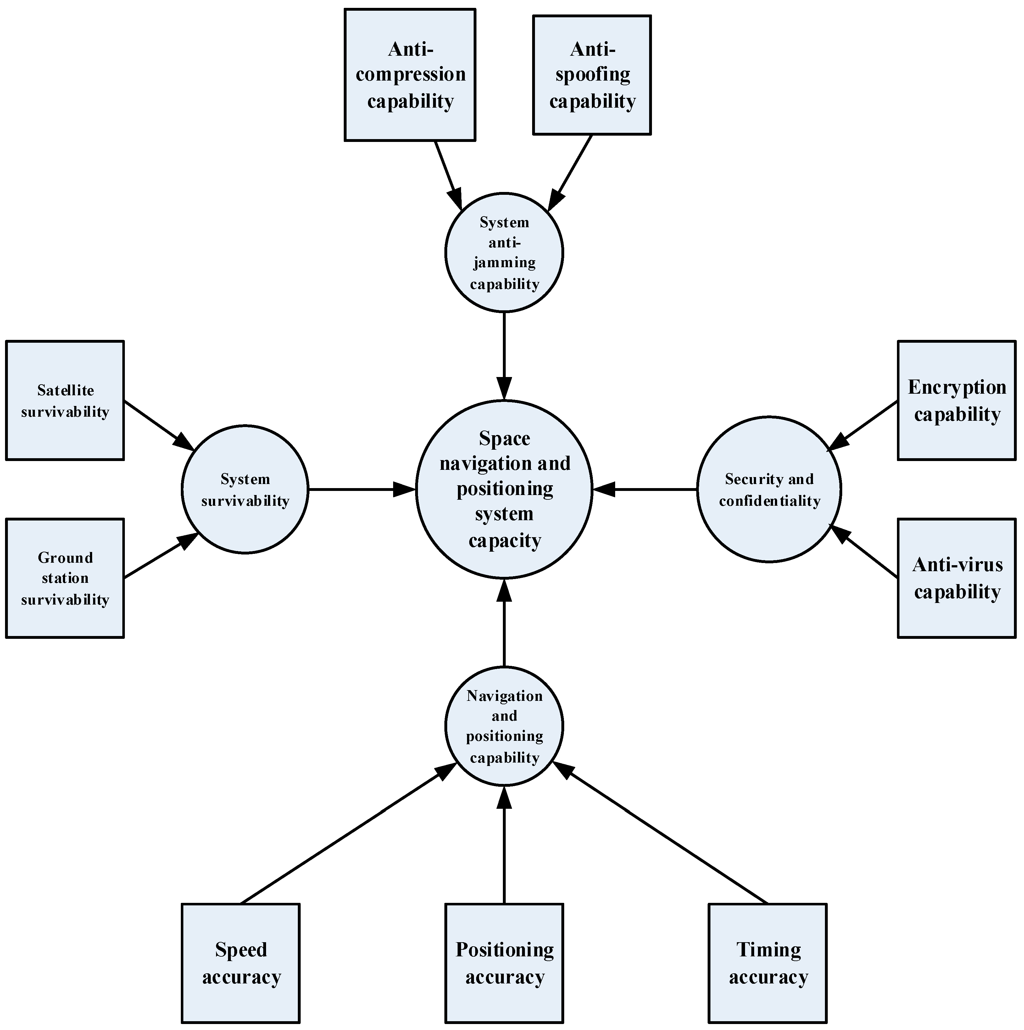
Figure 2.
Conditional-belief-parameter table for spatial navigation and positioning capabilities.
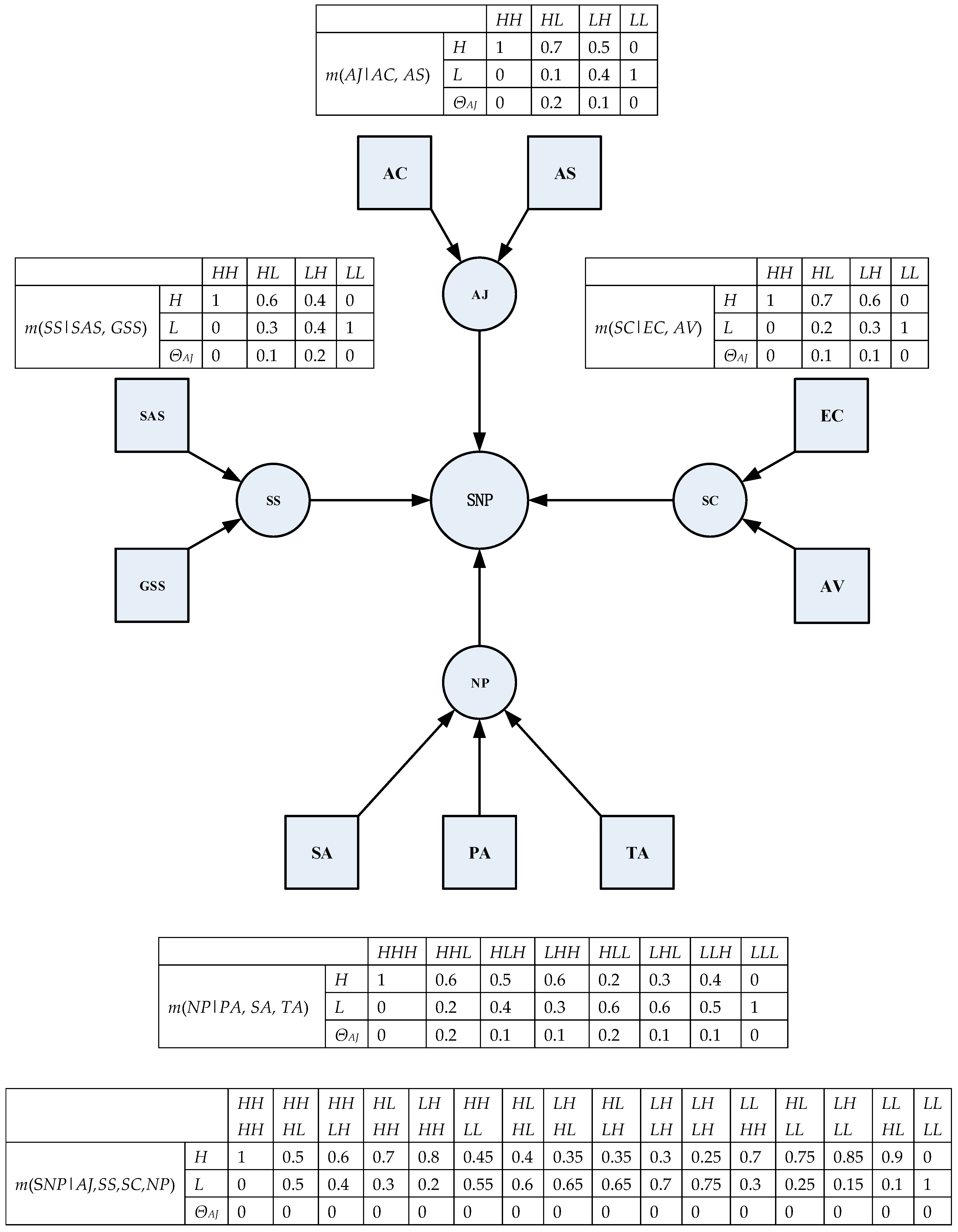
Figure 3.
The belief distribution of the requirement-satisfaction degree of each upper-layer capability.
Figure 3.
The belief distribution of the requirement-satisfaction degree of each upper-layer capability.
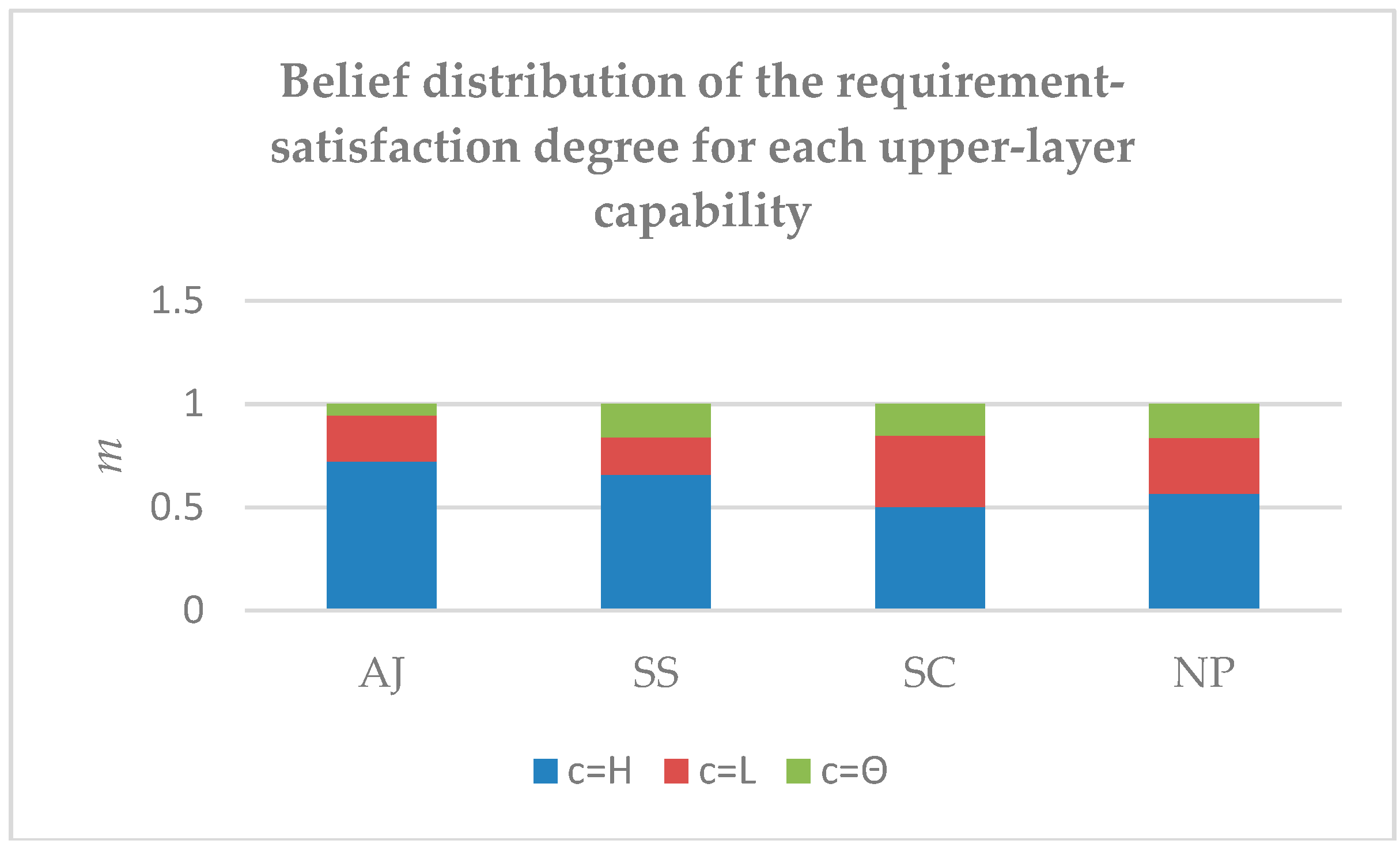
Figure 4.
Conditional probability distribution (CPD) of spatial navigation and positioning capabilities.
Figure 4.
Conditional probability distribution (CPD) of spatial navigation and positioning capabilities.

Figure 5.
A comparison of the results obtained through the two methods (Bayesian and evidential).
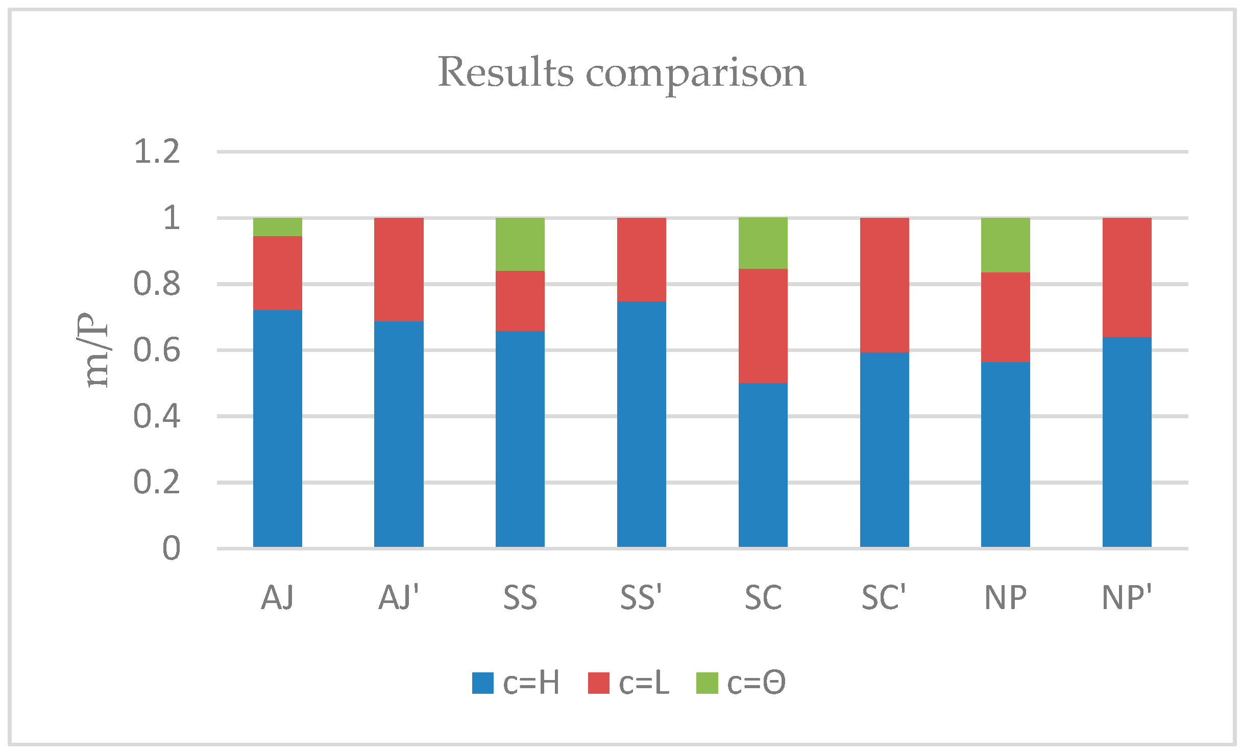
Figure 6.
Prioritization of capability gaps.
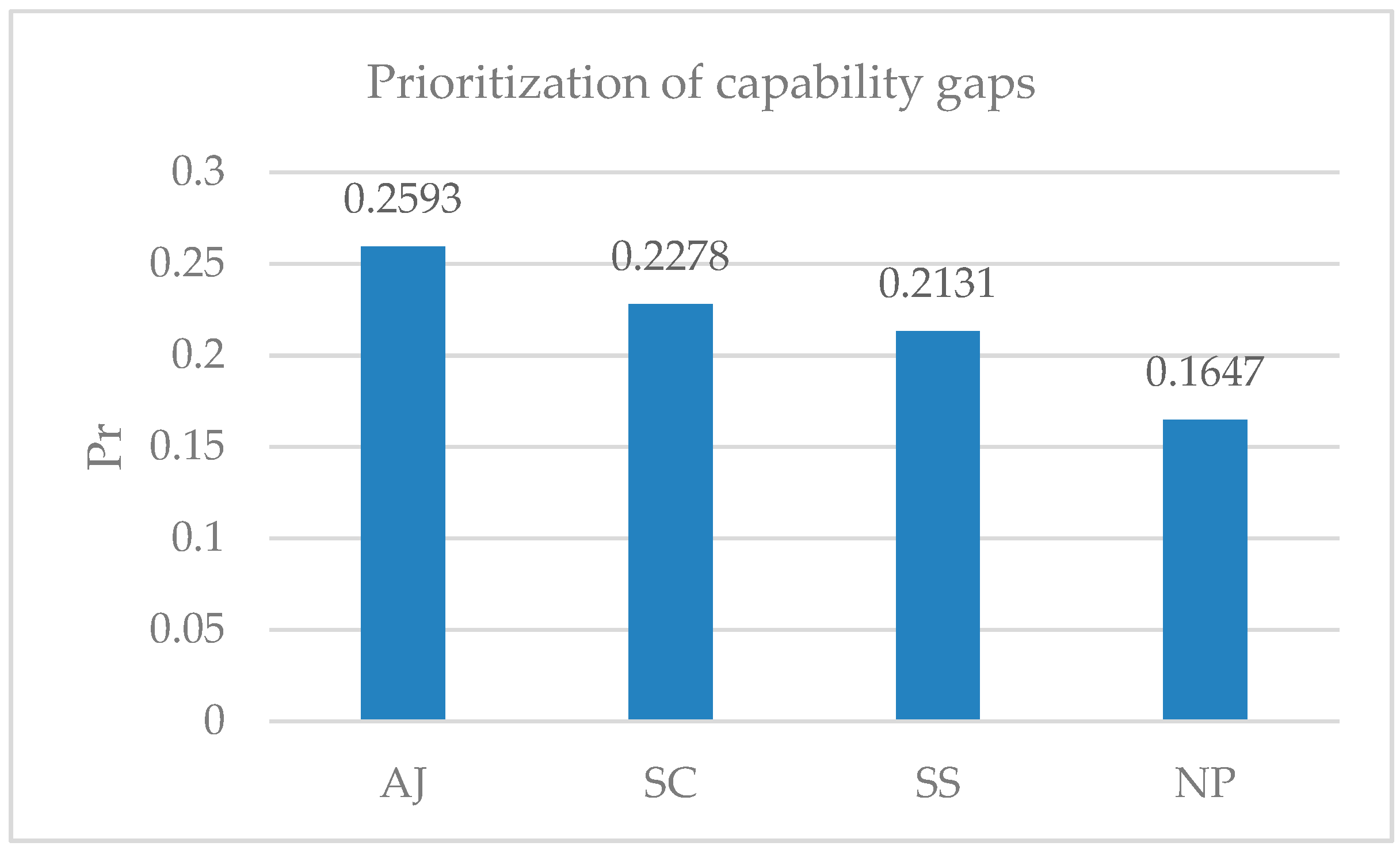
Figure 7.
Result analysis.

Table 1.
Identification framework for space navigation and positioning capabilities.
| Node | Recognition Frame Θ |
|---|---|
| Space-navigation-and-positioning system capability (SNP) | {high (H), medium (M), low (L)} |
| Anti-jamming capability (AJ) | {high, low} |
| Anti-compression capability (AC) | {high, low} |
| Anti-spoofing capability (AS) | {high, low} |
| System survivability (SS) | {high, low} |
| Satellite survivability (SAS) | {high, low} |
| Ground station survivability (GSS) | {high, low} |
| Security and confidentiality (SC) | {high, low} |
| Encryption capability (EC) | {high, low} |
| Anti-virus capability (AV) | {high, low} |
| Navigation and positioning capability (NP) | {high, low} |
| Positioning accuracy (PA) | {high, low} |
| Speed accuracy (SA) | {high, low} |
| Timing accuracy (TA) | {high, low} |
Table 2.
Capability parameters.
| Capability | Sub-Capabilities and Indicators | Weight | Ideal Value | Minimum Value | Actual Value | Credibility |
|---|---|---|---|---|---|---|
| Anti-jamming capability (0.15) | Anti-compression capability (dBc) | 0.6 | 120 | 50 | 90 | 1 |
| Anti-spoofing capability (dBc) | 0.4 | 100 | 40 | 90 | 1 | |
| System survivability (0.1) | Satellite survivability | 0.7 | 100 | 60 | 90 | 0.9 |
| Ground-station survivability | 0.3 | 100 | 60 | 80 | 0.9 | |
| Security and confidentiality (0.1) | Encryption capability | 0.5 | 100 | 50 | 70 | 0.9 |
| Anti-virus capability | 0.5 | 100 | 50 | 80 | 0.9 | |
| Navigation and positioning capability (0.65) | Positioning accuracy (m) | 0.4 | 5 | 20 | 10 | 0.95 |
| Speed accuracy (m/s) | 0.3 | 0.1 | 0.5 | 0.2 | 0.95 | |
| Timing accuracy (ns) | 0.3 | 10 | 100 | 50 | 0.95 |
Table 3.
The belief distribution of the degree of demand-satisfaction for bottom-capability indicators.
Table 3.
The belief distribution of the degree of demand-satisfaction for bottom-capability indicators.
| Bottom-Capability Indicators | m0 (c=H) | m0 (c=L) | m0 (Θ) |
|---|---|---|---|
| Anti-compression capability | 0.571 | 0.429 | 0 |
| Anti-spoofing capability | 0.833 | 0.167 | 0 |
| Satellite survivability | 0.675 | 0.225 | 0.1 |
| Ground station survivability | 0.45 | 0.45 | 0.1 |
| Encryption capability | 0.36 | 0.54 | 0.1 |
| Anti-virus capability | 0.54 | 0.36 | 0.1 |
| Speed accuracy | 0.7125 | 0.2375 | 0.05 |
| Timing accuracy | 0.528 | 0.422 | 0.05 |
Table 4.
The belief distribution of the requirement-satisfaction degree for each upper-layer capability.
Table 4.
The belief distribution of the requirement-satisfaction degree for each upper-layer capability.
| Capability | m (c=H) | m (c=M) | m (c=L) | m(Θ) |
|---|---|---|---|---|
| Anti-jamming capability | 0.7211 | - | 0.2241 | 0.0548 |
| System survivability | 0.6588 | - | 0.1816 | 0.1596 |
| Security and confidentiality | 0.5008 | - | 0.3460 | 0.1533 |
| Navigation and positioning capability | 0.5647 | - | 0.2714 | 0.1639 |
| Space-navigation-and-positioning system capability | 0.3567 | 0.1656 | 0.1699 | 0.3077 |
Table 5.
The prior probability of bottom capability indicators.
| Bottom Capability Indicators | P0 (c=H) | P0 (c=L) |
|---|---|---|
| Satellite survivability | 0.725 | 0.275 |
| Ground station survivability | 0.5 | 0.5 |
| Anti-compression capability | 0.571 | 0.429 |
| Anti-spoofing capability | 0.833 | 0.167 |
| Positioning accuracy | 0.658 | 0.342 |
| Speed accuracy | 0.7375 | 0.2625 |
| Timing accuracy | 0.543 | 0.447 |
| Encryption capability | 0.41 | 0.59 |
| Anti-virus capability | 0.59 | 0.41 |
Table 6.
The probability distribution of the requirement-satisfaction degree for each upper-layer capability.
Table 6.
The probability distribution of the requirement-satisfaction degree for each upper-layer capability.
| Capability | P (c=H) | P (c=M) | P (c=L) |
|---|---|---|---|
| Anti-jamming capability | 0.6875 | - | 0.3125 |
| System survivability | 0.7485 | - | 0.2515 |
| Security and confidentiality | 0.5942 | - | 0.4053 |
| Navigation and positioning capability | 0.6404 | - | 0.3596 |
| Space-navigation-and-positioning system capability | 0.4482 | 0.2745 | 0.2773 |
Table 7.
The reverse conditional likelihood functions.
| (AJ, SS, SC, NP) | HHHH | HHHL | HHLH | HLHH | LHHH | HHLL | HLHL | LHHL |
|---|---|---|---|---|---|---|---|---|
| Pl((AJ,SS,SC,NP)|SNP=L) | 0 | 0 | 0 | 0 | 0 | 0.55K | 0.6K | 0.65K |
| (AJ, SS, SC, NP) | HLLH | LHLH | LLHH | HLLL | LHLL | LLHL | LLLH | LLLL |
| Pl((AJ,SS,SC,NP)|SNP=L) | 0.65K | 0.7K | 0.75K | 0.7K | 0.75K | 0.85K | 0.9K | K |
© 2018 by the authors. Licensee MDPI, Basel, Switzerland. This article is an open access article distributed under the terms and conditions of the Creative Commons Attribution (CC BY) license (http://creativecommons.org/licenses/by/4.0/).
Share and Cite
MDPI and ACS Style
Pei, D.; Qin, D.; Sun, Y.; Bu, G.; Yao, Z. Prioritization Assessment for Capability Gaps in Weapon System of Systems Based on the Conditional Evidential Network. Appl. Sci. 2018, 8, 265. https://doi.org/10.3390/app8020265
AMA Style
Pei D, Qin D, Sun Y, Bu G, Yao Z. Prioritization Assessment for Capability Gaps in Weapon System of Systems Based on the Conditional Evidential Network. Applied Sciences. 2018; 8(2):265. https://doi.org/10.3390/app8020265
Chicago/Turabian StylePei, Dong, Daguo Qin, Yang Sun, Guangzhi Bu, and Zhonghua Yao. 2018. "Prioritization Assessment for Capability Gaps in Weapon System of Systems Based on the Conditional Evidential Network" Applied Sciences 8, no. 2: 265. https://doi.org/10.3390/app8020265
Note that from the first issue of 2016, this journal uses article numbers instead of page numbers. See further details here.