Identification of Operating Parameters Most Strongly Influencing the Jetting Performance in a Piezoelectric Actuator-Driven Dispenser


Abstract
:1. Introduction
- (1)
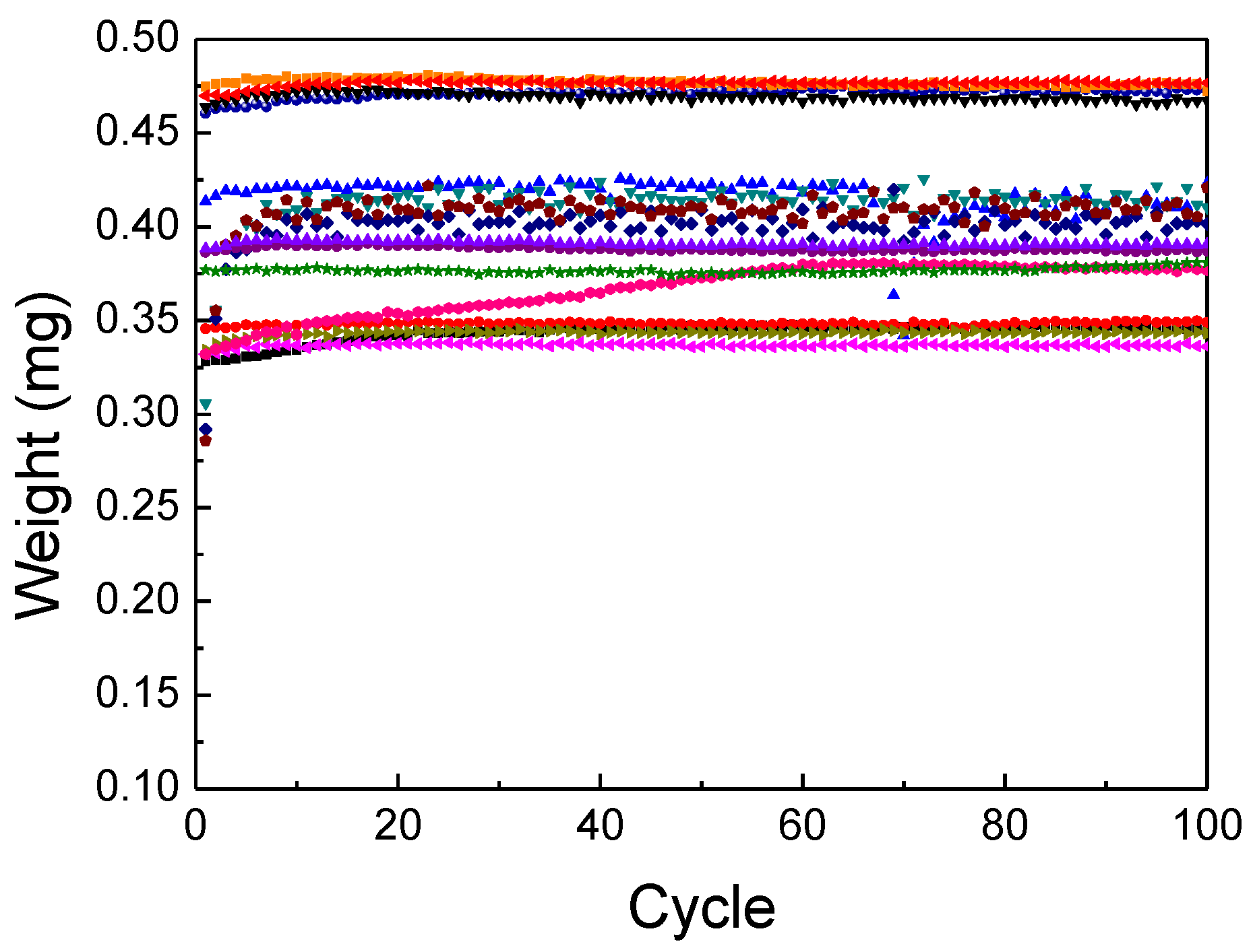
- The effects of practical operating parameters, such as the needle stroke, on the jetting performances are experimentally evaluated. In the test, special attention is required to avoid testing errors since the weight of a single dispensed dot should be repeatedly measured 100 times for each test.
- (2)
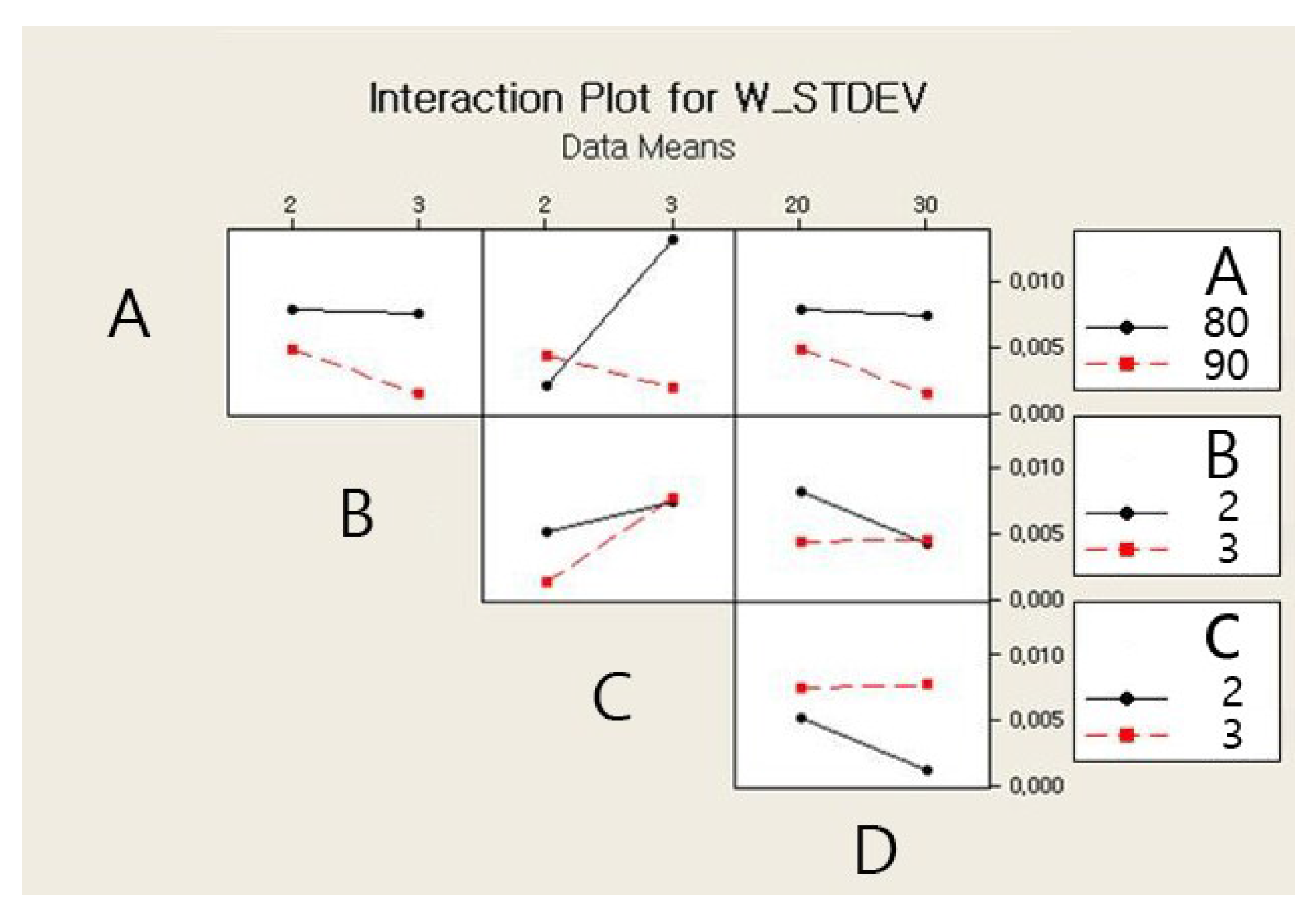
- The evaluated results are statistically analyzed to determine the optimal operating parameters that can be directly used in LED-packaging industrial fields. The statistical analysis identifies the effect of each operating parameter on the average and variance of the dispensing amount, and the effect of the interactions with other parameters is also investigated.
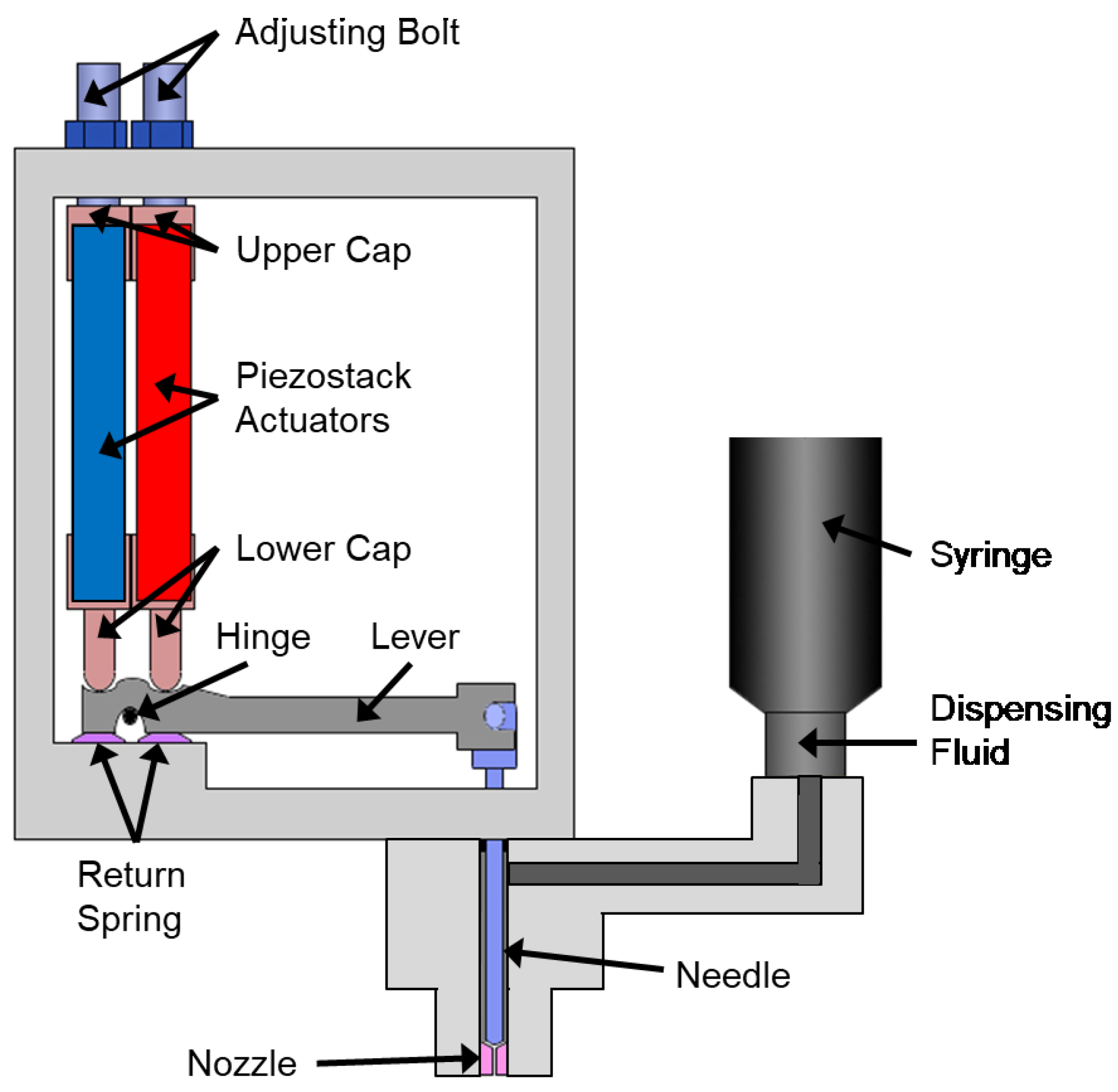
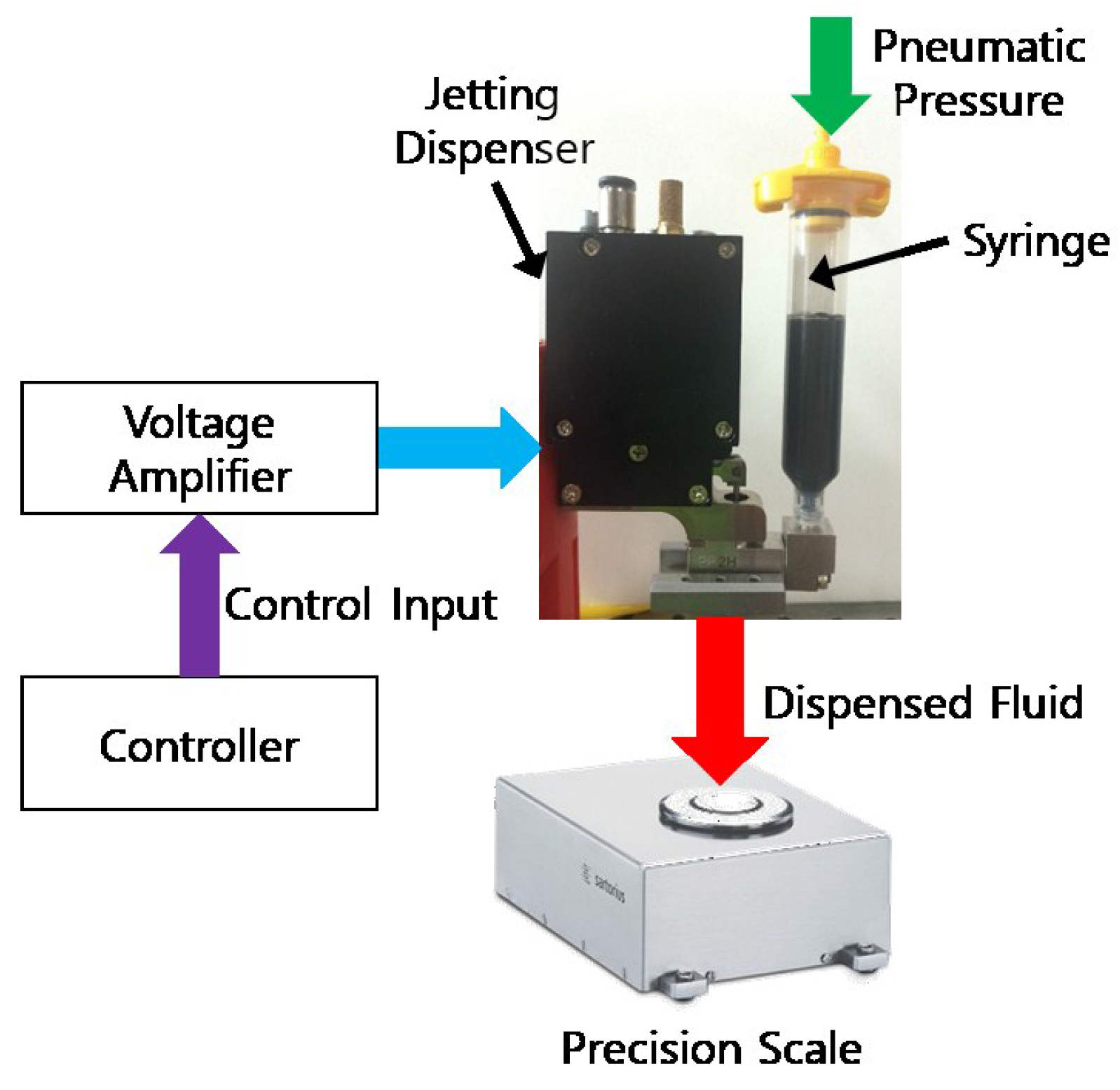
2. Dual Piezostack-Driven Jetting Dispenser
- (1)
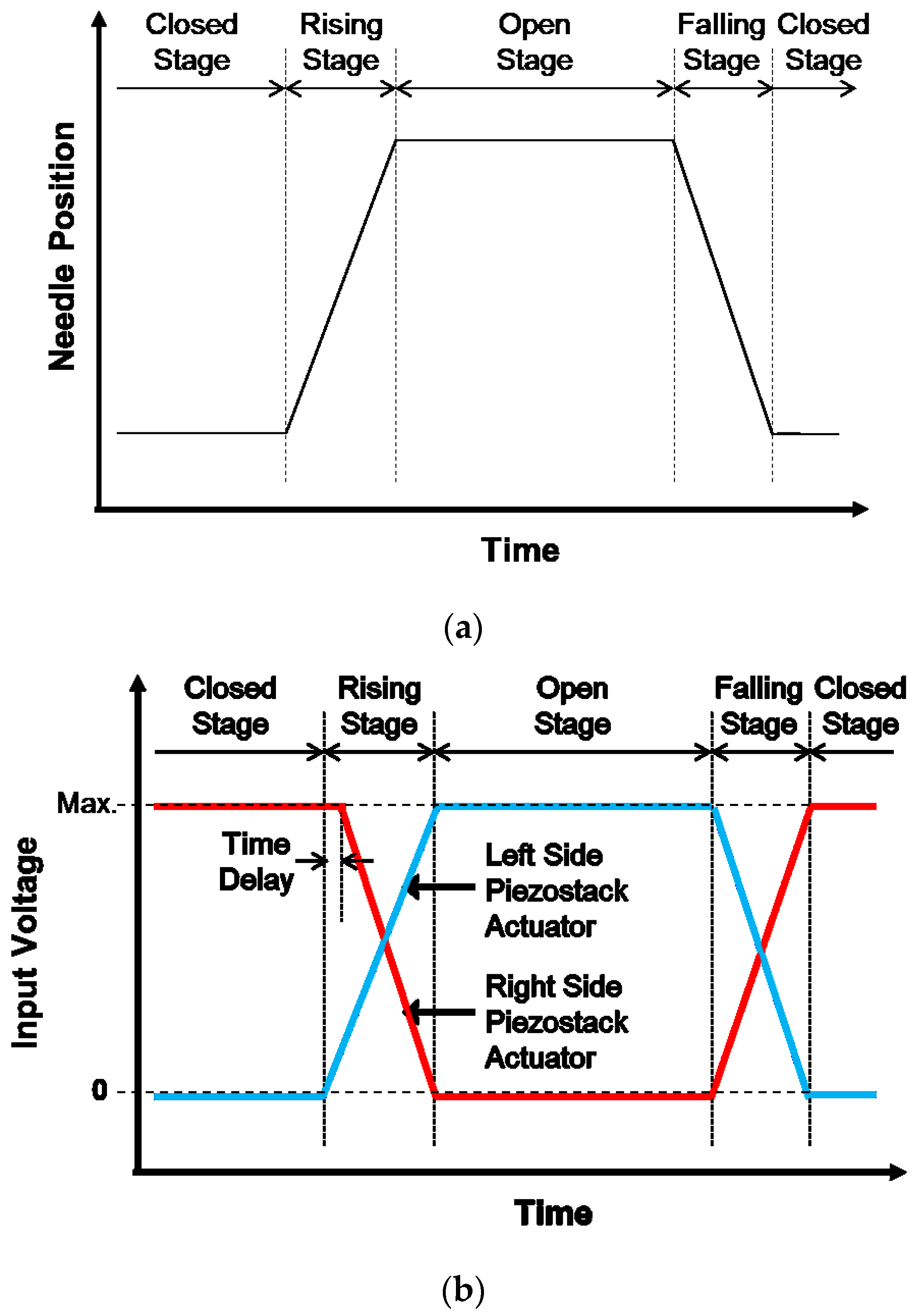
- Rising Stage: The lever rotates in a counterclockwise direction and the needle moves upward when the left- and right-side piezostack actuators are elongated and contracted, respectively. Subsequently, the fluid in the syringe begins to fill the empty space in the dispenser head.
- (2)
- Open Stage: The position of the needle is maintained by applying the proper control input voltage to obtain perfect filling of the dispensing fluid.
- (3)
- Falling Stage: The lever rotates in a clockwise direction and the needle moves downward when the left- and right-side piezostack actuators are contracted and elongated, respectively. The needle penetrates the fluid and dispenses it through the nozzle of the head by using the impact energy.
- (4)
- Closed Stage (delay): The position of the needle remains lowered until the next jetting operation.
3. Design of the Experimental Test
4. Results and Analysis
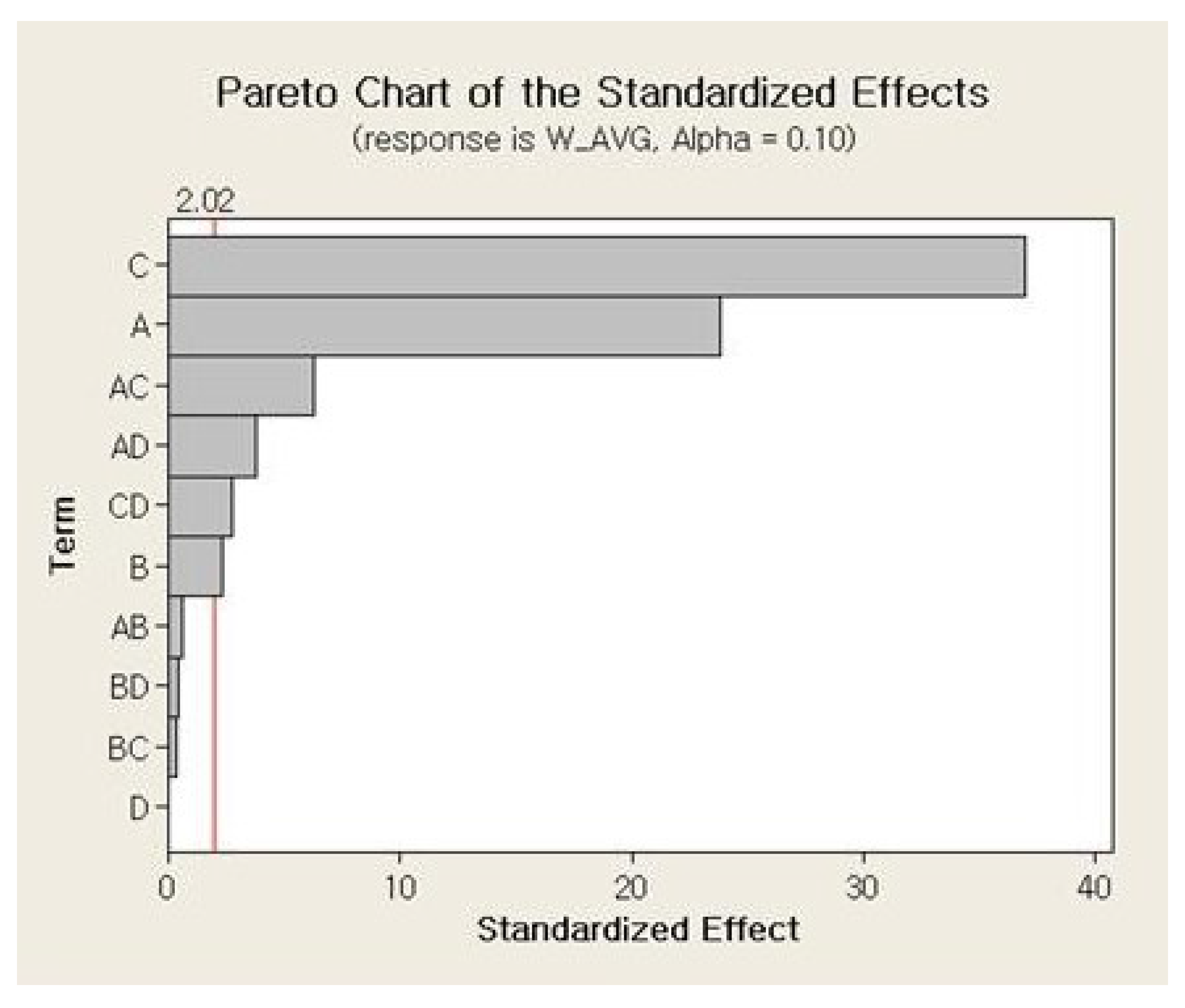
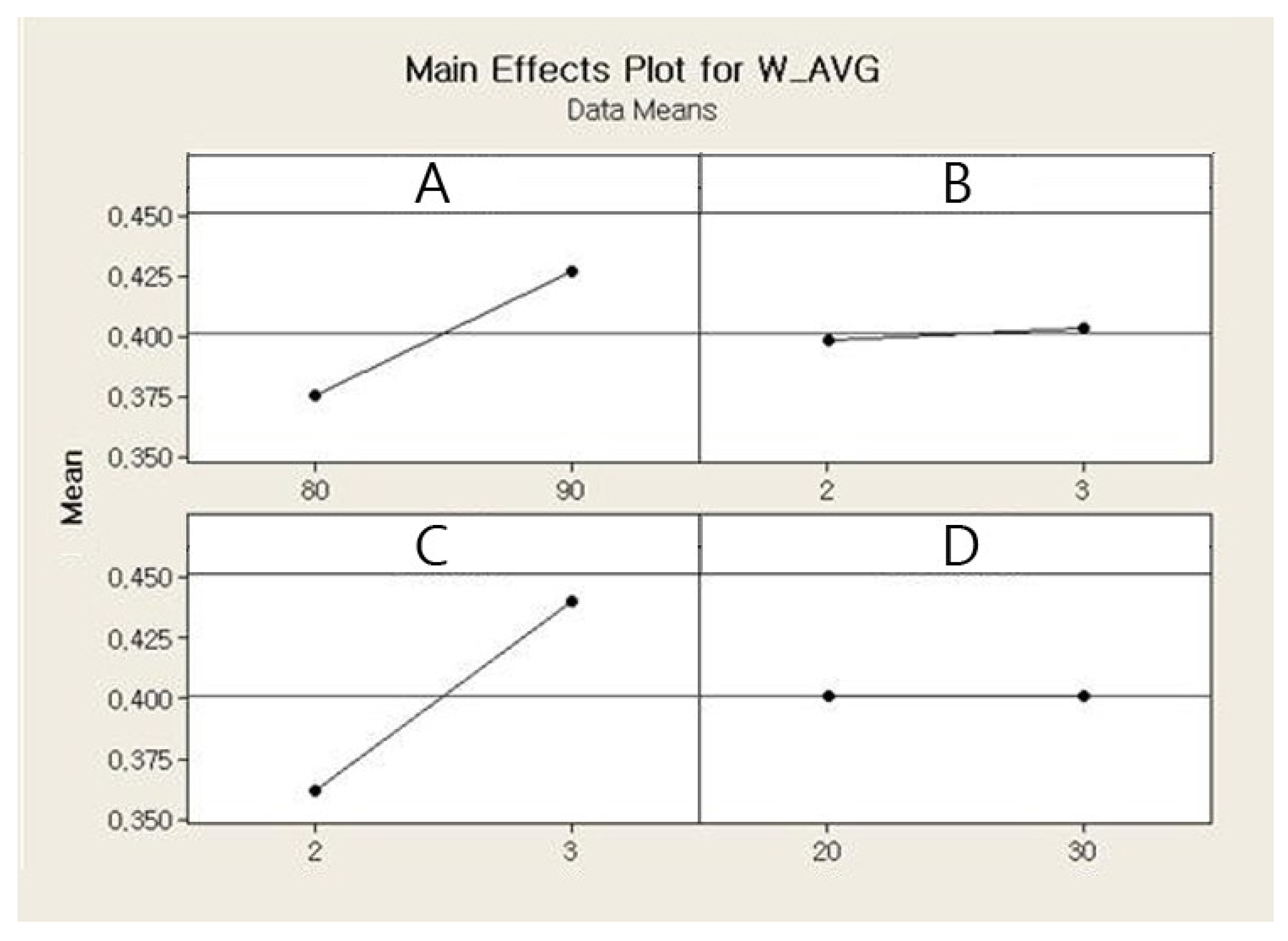
4.1. Average Weight
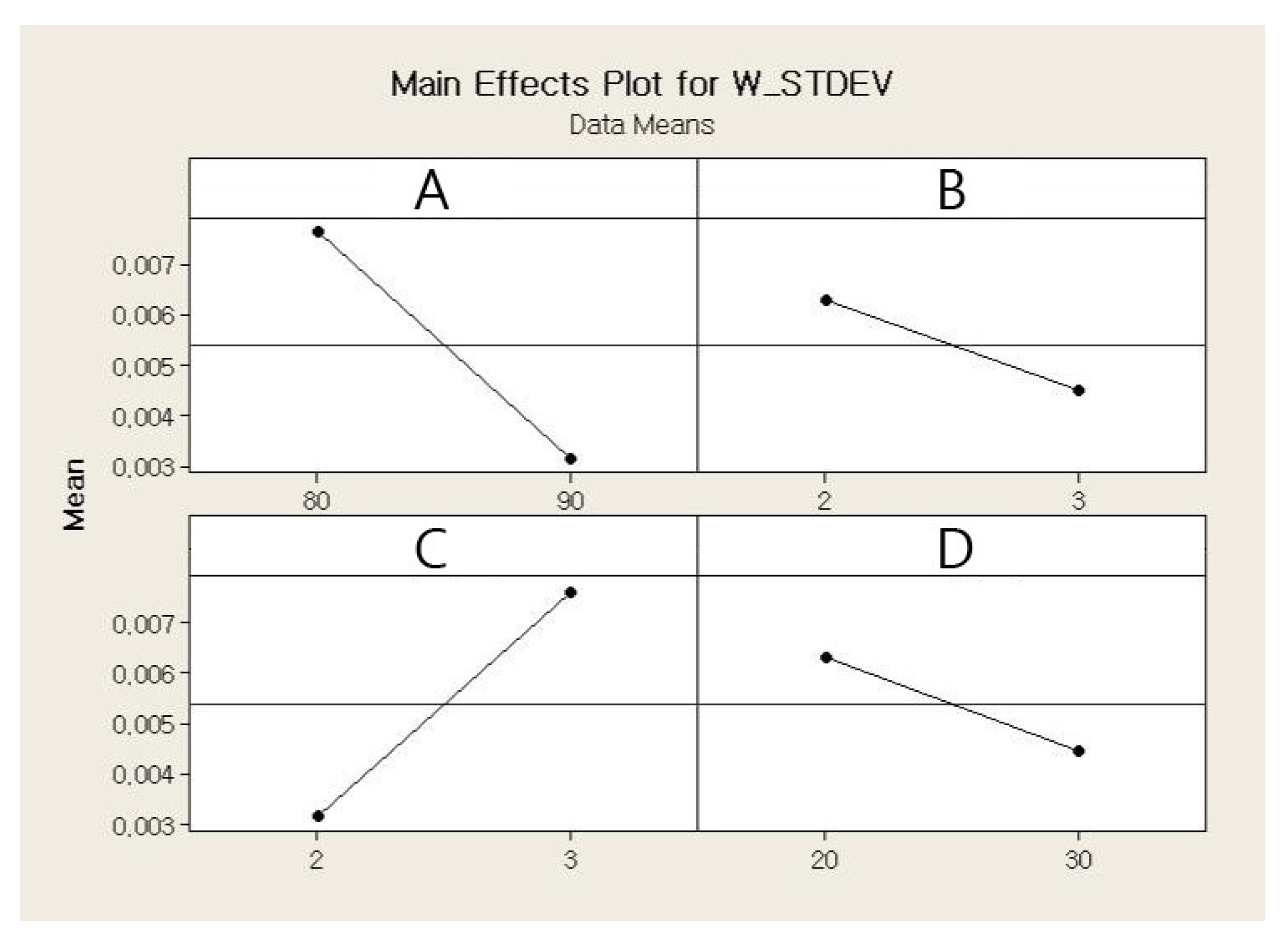
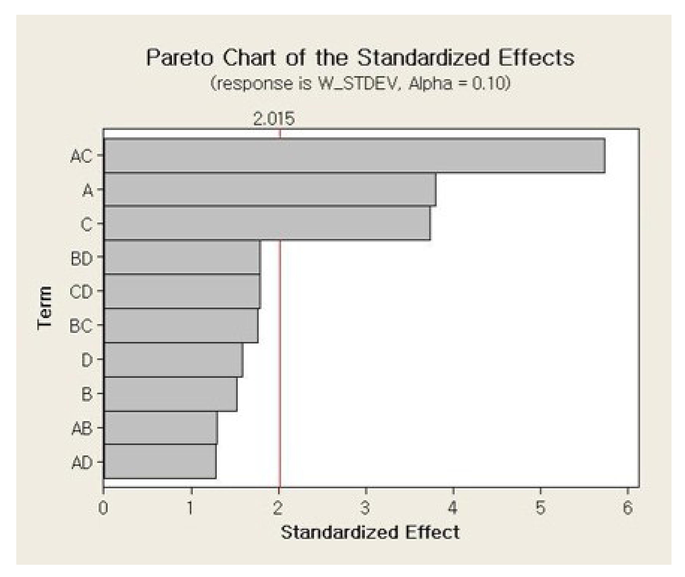
4.2. Weight Variation
5. Conclusions
Author Contributions
Conflicts of Interest
References
- Li, J.; Deng, G. Technology Development and Basic Theory Study of Fluid Dispensing—A Review. In Proceedings of the Sixth IEEE CPMT Conference on High Density Microsystem Design and Packaging and Component Failure Analysis, Shanghai, China, 30 June–3 July 2004; pp. 198–205. [Google Scholar]
- Nguon, B.; Jouaneh, M. Design and Characterization of a Precision Fluid Dispensing Valve. Int. J. Adv. Manuf. Technol. 2004, 24, 251–260. [Google Scholar] [CrossRef]
- Chen, X.B.; Kai, J. Modeling of Positive-Displacement Fluid Dispensing Process. IEEE Trans. Electron. Packag. Manuf. 2004, 27, 157–163. [Google Scholar] [CrossRef]
- Chen, X.B. Modeling of Rotary Screw Fluid Dispensing Processes. J. Electron. Packag. 2007, 129, 172–178. [Google Scholar] [CrossRef]
- Chen, C.P.; Li, H.X.; Ding, H. Modeling and Control of Time-pressure Dispensing for Semiconductor Manufacturing. Int. J. Autom. Comput. 2007, 4, 422–427. [Google Scholar] [CrossRef]
- Jia, H.; Hua, Z.; Li, M.; Zhang, J.; Zhang, J. A Jetting System or Chip on Glass Package. In Proceedings of the International Conference on Electronic Packaging Technology & High Density Packaging, Beijing, China, 10–13 August 2009; pp. 954–960. [Google Scholar]
- Ge, Z.; Deng, G. Design and Modeling of Jet Dispenser Based on Giant Magnetostrictive Material. In Proceedings of the International Conference on Electronic Packaging Technology & High Density Packaging, Beijing, China, 10–13 August 2009; pp. 974–979. [Google Scholar]
- Wang, L.; Du, J.; Luo, Z.; Du, X.; Li, Y.; Liu, J.; Sun, D. Design and Experiment of a Jetting Dispenser Driven by Piezostack Actuator. IEEE Trans. Electron. Packag. Manuf. 2013, 3, 147–156. [Google Scholar] [CrossRef]
- Luo, W.; Deng, G. Simulation Analysis of Jetting Dispenser Based on Two Piezoelectric Stacks. In Proceedings of the 14th International Conference on Electronic Packaging Technology (ICEPT), Dalian, China, 11–14 August 2013; pp. 738–741. [Google Scholar]
- Lu, S.; Liu, Y.; Yao, Y.; Huang, B.; Sun, L. Design and Analysis of a Piezostack Driven Jetting Dispenser for High Viscosity Adhesives. In Proceedings of the IEEE/ASME International Conference on Advanced Intelligent Mechatronics (AIM), Besacon, France, 8–11 July 2014; pp. 227–232. [Google Scholar]
- Lu, S.; Liu, Y.; Yao, Y.; Sun, L.; Zhong, M. Bond-graph Model of a Piezostack Driven Jetting Dispenser. Simul. Model. Pract. Theory 2014, 49, 193–202. [Google Scholar] [CrossRef]
- Nguyen, Q.H.; Choi, M.K.; Choi, S.B. A New Type of Piezostack-driven Jetting Dispenser for Semiconductor Electronic Packaging: Modeling and Control. Smart Mater. Struct. 2008, 17, 015033. [Google Scholar] [CrossRef]
- Nguyen, Q.H.; Choi, M.K.; Yun, B.Y.; Choi, S.B. Design of a Novel Jetting Dispenser Featuring Piezostack and Linear Pump. J. Intell. Mater. Syst. Struct. 2008, 19, 333–341. [Google Scholar] [CrossRef]
- Nguyen, Q.H.; Choi, S.B.; Kim, J.D. The Design and Control of a Jetting Dispenser for Semiconductor Electronic Packaging Driven by a Piezostack and a Flexible Beam. Smart Mater. Struct. 2008, 17, 065028. [Google Scholar] [CrossRef]
- Jeon, J.; Hong, S.M.; Choi, M.K.; Choi, S.B. Design and Performance Evaluation of a New Jetting Dispenser System Using Two Piezostack Actuators. Smart Mater. Struct. 2015, 24, 015020. [Google Scholar] [CrossRef]
- Hong, S.M. Fabrication and Characteristics of Jetting Dispenser with Dual Piezostack Actuators. Ph.D. Thesis, Department of Mechanical Engineering, Inha University, Busan, Korea, 2014. [Google Scholar]
- Uchino, K. Materials Issues in Design and Performance of Piezoelectric Actuators: An Overview. Acta Mater. 1998, 46, 3745–3753. [Google Scholar] [CrossRef]
- Luo, Q.; Tong, L. Design and Testing for Shape Control of Piezoelectric Structures using Topology Optimization. Eng. Struct. 2015, 97, 90–104. [Google Scholar] [CrossRef]
- Randall, C.A.; Kelnberger, A.; Yang, G.Y.; Eitel, R.E.; Shrout, T.R. High Strain Piezoelectric Multilayer Sctuators—A Material Science and Engineering Challenge. J. Electroceram. 2005, 14, 177–191. [Google Scholar] [CrossRef]
- Webber, K.G.; Vögler, M.; Khansur, N.H.; Kaeswurm, B.; Daniels, J.E.; Schader, F.H. Review of the mechanical and fracture behavior of perovskite lead-free ferroelectrics for actuator applications. Smart Mater. Struct. 2017, 26, 063001. [Google Scholar] [CrossRef]
- Minitab 17 Support. Available online: https://support.minitab.com/en-us/minitab/17 (accessed on 5 February 2018).


| Components | Parameter | Value |
|---|---|---|
| Lever | Distance from hinge to needle | 51.5 mm |
| Thickness | 4 mm | |
| Width | 10 mm | |
| Return Spring | Height | 0.6 mm |
| Outer Diameter | 8 mm | |
| Inner Diameter | 4.2 mm | |
| Hinge | Diameter | 2 mm |
| Parameter | Value |
|---|---|
| Dimensions | 5 × 5 × 40 mm |
| Blocking Force | 750 N |
| Maximum Displacement | 42 μm @ 150 V |
| Stiffness | 20.2 N/μm |
| Resonant Frequency | 34 kHz |
| Rising Time | 20.32 μs |
| Falling Time | 26.68 μs |
| Material | Property | Value | |
|---|---|---|---|
| Silicone (OE-6630) | Viscosity | 2300 cp | |
| Surface Tension | 2.2 × 10⁻⁶ N/cm | ||
| Density | Part A | 1.10 g/cm3 | |
| Part B | 1.15 g/cm3 | ||
| Phosphor (YAG) | Density | 4.40 g/cm3 | |
| Mixture (Part A:Part B = 1:1 and Phosphor 15%) | Density | 1.20 g/cm3 | |
| Notation | Parameter | Unit | Level 1 | Level 2 |
|---|---|---|---|---|
| A | Needle Stroke | % | 80 | 90 |
| B | Rising Time | ms | 2 | 3 |
| C | Open Time | ms | 2 | 3 |
| D | Cooling Pressure | kPa | 138 | 207 |
| Run | Needle Stroke (%) | Rising Time (ms) | Open Time (ms) | Cooling Pressure (kPa) |
|---|---|---|---|---|
| 1 | 80 | 2 | 2 | 138 |
| 2 | 80 | 3 | 2 | 138 |
| 3 | 80 | 2 | 3 | 138 |
| 4 | 80 | 3 | 3 | 138 |
| 5 | 80 | 2 | 2 | 207 |
| 6 | 80 | 3 | 2 | 207 |
| 7 | 80 | 2 | 3 | 207 |
| 8 | 80 | 3 | 3 | 207 |
| 9 | 90 | 2 | 2 | 138 |
| 10 | 90 | 3 | 2 | 138 |
| 11 | 90 | 2 | 3 | 138 |
| 12 | 90 | 3 | 3 | 138 |
| 13 | 90 | 2 | 2 | 207 |
| 14 | 90 | 3 | 2 | 207 |
| 15 | 90 | 2 | 3 | 207 |
| 16 | 90 | 3 | 3 | 207 |
| Run | Average (mg) | Standard Deviation |
|---|---|---|
| 1 | 0.344 | 0.005 |
| 2 | 0.348 | 0.001 |
| 3 | 0.416 | 0.012 |
| 4 | 0.412 | 0.013 |
| 5 | 0.337 | 0.001 |
| 6 | 0.343 | 0.001 |
| 7 | 0.400 | 0.013 |
| 8 | 0.407 | 0.014 |
| 9 | 0.367 | 0.014 |
| 10 | 0.377 | 0.001 |
| 11 | 0.471 | 0.003 |
| 12 | 0.477 | 0.002 |
| 13 | 0.388 | 0.001 |
| 14 | 0.391 | 0.001 |
| 15 | 0.469 | 0.002 |
| 16 | 0.476 | 0.002 |
| Parameter | Effect | Coeff. | SE Coeff. | t | p |
|---|---|---|---|---|---|
| Const. | - | 4.01406 | 0.01075 | 373.52 | 0.000 |
| A | 0.51148 | 0.25574 | 0.01075 | 23.80 | 0.000 |
| B | 0.05073 | 0.02536 | 0.01075 | 2.36 | 0.065 |
| C | 0.79355 | 0.39677 | 0.01075 | 36.91 | 0.000 |
| D | 0.00076 | 0.00038 | 0.01075 | 0.04 | 0.973 |
| AB | 0.01231 | 0.00615 | 0.01075 | 0.57 | 0.592 |
| AC | 0.13426 | 0.06713 | 0.01075 | 6.25 | 0.002 |
| AD | 0.08204 | 0.04102 | 0.01075 | 3.82 | 0.012 |
| BC | −0.00793 | −0.00396 | 0.01075 | −0.37 | 0.727 |
| BD | 0.00876 | 0.00438 | 0.01075 | 0.41 | 0.701 |
| CD | −0.05845 | −0.02922 | 0.01075 | −2.72 | 0.042 |
| Parameter | Effect | Coeff. | SE Coeff. | t | p |
|---|---|---|---|---|---|
| Const. | - | 4.01406 | 0.009015 | 445.26 | 0.000 |
| A | 0.51148 | 0.25574 | 0.009015 | 28.37 | 0.000 |
| B | 0.05073 | 0.02536 | 0.009015 | 2.81 | 0.023 |
| C | 0.79355 | 0.39677 | 0.009015 | 44.01 | 0.000 |
| AC | 0.13426 | 0.06713 | 0.009015 | 7.45 | 0.000 |
| AD | 0.08204 | 0.04102 | 0.009015 | 4.55 | 0.002 |
| CD | −0.05845 | −0.02922 | 0.009015 | −3.24 | 0.012 |
| Parameter | Effect | Coeff. | SE Coeff. | t | p |
|---|---|---|---|---|---|
| Const. | - | 0.05403 | 0.005927 | 9.12 | 0.000 |
| A | −0.04508 | −0.02254 | 0.005927 | −3.80 | 0.013 |
| B | −0.01808 | −0.00904 | 0.005927 | −1.53 | 0.188 |
| C | 0.04427 | 0.02213 | 0.005927 | 3.73 | 0.014 |
| D | −0.01883 | −0.00941 | 0.005927 | −1.59 | 0.173 |
| AB | −0.01528 | −0.00764 | 0.005927 | −1.29 | 0.254 |
| AC | −0.06796 | −0.03398 | 0.005927 | −5.73 | 0.002 |
| AD | −0.01509 | −0.00755 | 0.005927 | −1.27 | 0.259 |
| BC | 0.02088 | 0.01044 | 0.005927 | 1.76 | 0.138 |
| BD | 0.02119 | 0.01059 | 0.005927 | 1.79 | 0.134 |
| CD | 0.02110 | 0.01055 | 0.005927 | 1.48 | 0.135 |
| Parameter | Effect | Coeff. | SE Coeff. | t | p |
|---|---|---|---|---|---|
| Const. | - | 0.05403 | 0.008133 | 6.64 | 0.000 |
| A | −0.04508 | −0.02254 | 0.008133 | −2.77 | 0.013 |
| C | 0.04427 | 0.02213 | 0.008133 | 2.72 | 0.019 |
| AC | −0.06796 | −0.03398 | 0.008133 | −4.18 | 0.001 |
© 2018 by the authors. Licensee MDPI, Basel, Switzerland. This article is an open access article distributed under the terms and conditions of the Creative Commons Attribution (CC BY) license (http://creativecommons.org/licenses/by/4.0/).
Share and Cite
Sohn, J.W.; Choi, S.-B. Identification of Operating Parameters Most Strongly Influencing the Jetting Performance in a Piezoelectric Actuator-Driven Dispenser. Appl. Sci. 2018, 8, 243. https://doi.org/10.3390/app8020243
Sohn JW, Choi S-B. Identification of Operating Parameters Most Strongly Influencing the Jetting Performance in a Piezoelectric Actuator-Driven Dispenser. Applied Sciences. 2018; 8(2):243. https://doi.org/10.3390/app8020243
Chicago/Turabian StyleSohn, Jung Woo, and Seung-Bok Choi. 2018. "Identification of Operating Parameters Most Strongly Influencing the Jetting Performance in a Piezoelectric Actuator-Driven Dispenser" Applied Sciences 8, no. 2: 243. https://doi.org/10.3390/app8020243
APA StyleSohn, J. W., & Choi, S.-B. (2018). Identification of Operating Parameters Most Strongly Influencing the Jetting Performance in a Piezoelectric Actuator-Driven Dispenser. Applied Sciences, 8(2), 243. https://doi.org/10.3390/app8020243