Article

Optimal Selection of Clustering Algorithm via Multi-Criteria Decision Analysis (MCDA) for Load Profiling Applications

by
Ioannis P. Panapakidis
1,* and
Georgios C. Christoforidis
2
1
Department of Electrical Engineering, Technological Educational Institute of Thessaly, 41110 Larisa, Greece
2
Department of Electrical Engineering, Western Macedonia University of Applied Sciences, 50100 Kozani, Greece
*
Author to whom correspondence should be addressed.
Appl. Sci. 2018, 8(2), 237; https://doi.org/10.3390/app8020237
Submission received: 3 January 2018 / Revised: 28 January 2018 / Accepted: 31 January 2018 / Published: 4 February 2018
(This article belongs to the Section Energy Science and Technology)

Abstract

:
Due to high implementation rates of smart meter systems, considerable amount of research is placed in machine learning tools for data handling and information retrieval. A key tool in load data processing is clustering. In recent years, a number of researches have proposed different clustering algorithms in the load profiling field. The present paper provides a methodology for addressing the aforementioned problem through Multi-Criteria Decision Analysis (MCDA) and namely, using the Technique for Order of Preference by Similarity to Ideal Solution (TOPSIS). A comparison of the algorithms is employed. Next, a single test case on the selection of an algorithm is examined. User specific weights are applied and based on these weight values, the optimal algorithm is drawn.

1. Introduction

1.1. Motivation

Among the key targets of Smart Grid’s operation is to bring forth new opportunities for the end consumers [1,2]. In traditional power systems, the consumers have zero or limited information about the actions that take place in electricity markets [3]. In order to upgrade the role of the consumer in the new landscape of power systems, it is essential to measure the load consumption and implement tools for information retrieval [4,5]. Smart metering infrastructure provides discrete time interval metering and, generally, more detailed data in terms of time resolution is available [6,7]. The processing of the collected load data can lead to the determination of consumers’ load profiles [8]. The term “load profiling” refers to the formulation of representative load curves over a given time period of a single consumer or groups of consumers [9,10,11]. The representative load curves or load profiles are actually the averaged load curves that have been grouped together in the same cluster. It should be noted that criteria such as voltage level, demographic parameters, type of economic activity, location and others are not sufficient enough to support a solid consumer classification [12]. This fact is recognized by current research leading to the examination of alternative methods to form consumer classes and derive the load profiles of each class [13].
Clustering is an unsupervised machine learning tool with proven performance in a wide variety of problems [14,15,16]. In recent years, many researchers have proposed clustering algorithms in the field of load profiling. A clustering algorithm is a tool for data processing and information retrieval. The data processing may refer to non-typical data detection and discarding. The load data are grouped together based on their similarity. The load profiles of the load data clusters are actually a descriptive model of the recorded load data. The amount of data can be represented by a reduced set of typical load curves or load profiles. Therefore, clustering-based load profiling can serve as the basic tool for processing of smart meter data. This fact is recognized in power systems community leading to an intense research effort to test algorithms for load data clustering [17]. However, while the load profiling literature is rich with implementations of clustering algorithms, there is no study that provides a general framework that reaches safe conclusions for algorithm selection. The aim of the present paper is not only to provide a detailed comparative analysis of the most commonly used algorithms in the literature and based on this analysis and to identify and discuss the benefits and drawbacks of each algorithm category but to rank the algorithms of the literature from the most to less efficient.

1.2. Solution Approach

The performance of a clustering algorithm is checked either with qualitative or quantitative criteria [17,18]. In the qualitative assessment, different algorithms are compared based on the shapes of the generated load profiles and the clustering compositions, i.e., the number of patterns that belong to each cluster. This assessment does not rely on mathematical objective criteria and is a minority in the literature. The quantitative assessment is based on the scores of the algorithm in a set of adequacy measures or clustering validity indicators. These indicators are built upon the Euclidean distance metric and evaluate the capacity of an algorithm to formulate well-separated and compact clusters. This assessment approach is the most common in the literature. However, while a clustering validity indicator provides a strong mathematical basis to build upon the conclusions derived from load profiling, the process of the evaluation of an algorithm is actually validity indicator specific. This means that the selection of an indicator influences the conclusions. For instance, a comparison of the algorithms with 2 different indicators can lead to different algorithms ranking. In order to deal with this issue, the present paper presents a set of 5 overarching criteria that can assess the complexity of an algorithm, its capacity per application and availability. These criteria are the following:
  • Criterion#1: Minimum number of parameters that need to be specified.
  • Criterion#2: Minimum requirement for parameter updating.
  • Criterion#3: Superior performance as measured by the most validity indicators.
  • Criterion#4: High execution speed/minimum time requirement.
  • Criterion#5: Generation of exploitable information about load data clusters.
  • Criterion#6: Software availability.
This paper implements the algorithms’ comparison as a multi-criteria decision-making problem, using the above criteria. We employ the Technique for Order of Preference by Similarity to Ideal Solution (TOPSIS) method to indicate which algorithm performs better at all the aforementioned criteria [19]. TOPSIS is a well-tested method in decision making; it is characterized by simplicity and flexibility, i.e., different distance metrics can be regarded to calculate the similarities between the alternative solutions and the ideal ones.

1.3. Literature Survey and Contributions

Two general models of load profiling are considered by utilities, namely the area based model and the category based model [20]. The area based model is adopted when there is not sufficient number of smart meter installations. Within a territory, at every time interval the consumption of consumers with smart meters (i.e., usually industrial consumers) is subtracted by the total (i.e., distribution transformer readings) and the remaining curve is deemed to the rest consumers with conventional meters. The area based model is appropriate in cases with low availability of data and high meter installation cost. The requirements of IT infrastructure (i.e., hardware, communication protocols, etc.) are lower compared to the category based model. However, it shortfalls in terms of accuracy, since it provides a simplified approach to load profile extraction. The category based model requires a considerable number of smart meters and a long period of systematic measurements. After the data collection, a data mining process takes place to formulate the load profiles. The process may refer to statistical analysis or to the implementation of clustering algorithms. For instance, static profiles are derived from existing historic data. The data classes are a priori known. If the data sample is sufficient then an average profile is extracted that represents the pre-defined class. Usually, the criterion for the classes’ formation is the type of electricity tariff. Static profiles formation does not require continuous measurements and averaging. Dynamic profiles refer to periodically updating the static profiles and adjusting them by taking into account temperature variations and other factors that affect the demand in daily or seasonal basis [21,22].
Load data profile generation is accomplished by load survey studies and clustering algorithms. Apart from consumption data, load surveys seek to gather weather data, consumer preferences, occupancy behaviour and others [23,24]. The accuracy of load surveys depends on the characteristics of the eligible sample of consumers [25,26]. Following a bottom-up-approach, the findings of load surveys on the eligible set are scaled up to include the rest consumers. This fact makes the clustering approach more flexible; different algorithms can be tested and no information on number of clusters is necessary. Also, the clustering approach requires only load data. While other variables such as temperature, tariff type and others may be incorporated in clusters, they are not mandatory.
Clustering-based load profiling is a multi-stage process [27,28]. The first stage refers to data cleansing, i.e., erroneous values detection and removal, missing data filling and others. Next, the 1st stage clustering takes place. For each consumer separately, the set with the daily load curves is clustered. The average daily load of each cluster is actually the normalized load profile. A specific load profile is chosen for each consumer and a second clustering occurs on the selected load profiles to produce the consumer classes. Therefore, the 1st stage clustering is held using the available daily load curves of each consumer and the 2nd stage clustering uses the load profiles derived from the previous stage. The final consumer clusters and the consumer clusters load profiles is the product of the 2nd stage. Note that the 1st stage clustering can be avoided [29]. In this case, the load profile that will represent the consumer refers to the average daily load curve of the consumer’s daily load curve set. These two stages can utilize one or more clustering algorithms. The algorithms that have been proposed in the related literature can be divided to the following categories: (a) Partitional algorithms such as the K-means, K-medoids and others; (b) hierarchical agglomerative algorithms such as the Ward’s algorithm and others; (c) fuzzy algorithms, such as the Fuzzy C-Means (FCM) and others (d) neural network based algorithms such as the Self-Organizing Map (SOM), Hopfield neural network and others and (e) algorithms that do not belong to the above classes, such as the Support Vector Clustering (SVC), the modified “follow-the-leader” (FDL), Renyi Entropy Clustering and others [11,17,18,19,20,21,22,23,24,25,26,27,28,29,30,31,32,33,34,35,36,37,38,39,40,41,42,43,44,45,46,47,48,49,50,51,52,53,54,55,56,57,58,59,60,61,62,63,64,65,66,67,68,69,70,71,72,73,74,75,76,77,78]. The algorithms differ in terms of efficiency, computational complexity, speed and others. The performance of an algorithm is evaluated by a set of clustering validity indicators [17]. In the majority of load profiling problems, the number of clusters is not known, i.e., external expertise information is absent. Therefore, a load profiling problem can be viewed as purely unsupervised machine learning task. This means that an algorithm should be executed for different number of clusters. For each number, the score on the validity indicator is checked. The clustering process is data driven and thus, external norms have to be considered to obtain the optimal number of clusters. A validity indicator is used for this purpose. It should be noted that increasing the number of clusters leads to better clustering. Yet, a high number of clusters is not preferable since it corresponds to increased complexity on the exploitation of clustering results. For example, a large number of consumer clusters may lead to difficulties in tariff design. On the other hand, a small number is also not desirable since it refers to poor clustering, i.e., high clustering errors. The data may refer to public buildings, a mix of residential, commercial and industrial consumers, single consumers, distribution feeders and others.
The existing works in the literature can be distinguished into 2 general types: The 1st type refers to the sole application of a clustering algorithm, while the 2nd type refers to a comparative analysis of algorithms of different type.
The sole application of the K-means algorithm is tested in [30]. The scope is to formulate the seasonal load profiles of 103 residential consumers with data measured per minute and covering a period of a full year. The results of the K-means are combined with homeowner’s survey data in order to track correlations between the consumption and other parameters like income, education level and others. In [31], the authors propose via the K-means the concept of dynamic clustering in Spanish residential consumers. This refers to clustering the full load time series (i.e., the total load sequence) instead of using daily curves. In [32], the data under examination are obtained from metering systems of a large utility in South Korea. The K-means is applied separately to the data corresponding to different consumer types such as residential, general high-voltage, industrial high-voltage and others. The optimal number of clusters per category varies. The study also includes a statistical analysis to obtain some key information of the consumption per cluster. In [33], the data set includes a set of households that is charged with time-of-use rates and another set with real-time pricing tariffs. The authors apply the principal component analysis to derive the principal components of household variables like solar heating, number of persons, building age and others. The K-means is applied in the set of principal components to cluster the variables and track households with similar variables.
Hierarchical agglomerative clustering is used in [34,35]. In [34], the single distance hierarchical algorithm is applied to the daily load curves of a Brazilian hospital. The purpose is to classify the load curves in clusters and afterwards employ a statistical analysis per clusters in order to gather information about the demand patterns and consumption levels per cluster. The scope is to exploit the load profiling outcome to build an energy management system for the hospital. In [35], the authors propose a new load data representation technique different from the time-domain one, using symbolic representation of the demand (i.e., letter characters). While the proposed representation technique seems promising in terms of expressing the daily load curves with a reduced set of features, it does not provide the optimal results in terms of low clustering compared with Sammon mapping, principal component analysis and others.
Fuzzy clustering is a generalization of crisp or hard clustering; the patterns (i.e., load curves) are distributed in all clusters with membership degrees that express partial membership. This fact provides flexibility in cluster structure and definition. The FCM algorithm is considered in [36] to cluster a set of load curves of distribution feeders in Malaysia that cover the needs of various domestic, commercial and small size industries consumers. The FCM performance is checked by 2 validity indicators. The same data set and algorithm are examined in [37]. The data refer to aggregated feeder loads and thus, no large differences in the shapes of the load profiles of the different clusters are observed. After the initial execution of the FCM, the algorithm is executed again separately in the daily load curves of each cluster. This leads to the formation of an additional load profile per cluster, a fact that increases the final number of load profiles. In [38], the FCM is checked with 7 clustering validity indicators. The algorithm is applied to the daily load curves that cover a period of a full year and correspond to the consumption of a city located in China. According to the paper’s findings, the value of the fuzziness parameter holds an important role in the FCM operation. This parameter is data specific, a fact that raise the need for several trial-and-error executions for its calibration. In [39], the authors investigate the influence of the fuzziness parameter in the FCM clustering outcome via a trial and error approach.
According to the results, the increment of the parameter results in lower clustering errors. In [40], the experiments include different execution of the FCM in order to calibrate the fuzziness parameters. The results indicate that while the value increases, the clustering error, as measured by 3 validity indicators, decreases. In [41], the set contains 124 daily load curves of an educational building in Spain. The FCM is used to cluster the data. The emphasis of the paper is placed on similarity metrics on the clustering validation. The authors experiment with different similarity metrics such as Mahalanobis distance, Dynamic Time Wrapping distance and others and conclude that the type of the metric considerably influence the results. Another trend in the related literature is to combine the FCM with supervised machine learning algorithm and namely, artificial neural networks. The general approach is to assign the load profiles generated by the FCM to pre-defined types of consumers or activities. More specifically, in [42] a number of pre-defined consumer types is present. The FCM clusters the data and later a Probabilistic Neural Network (PNN) is used to classify the load profiles drawn by the FCM to the consumer types. In [43], the FCM is again combined with the PNN. The load profiles obtained by the FCM are used to train the PNN. The latter is used to categorize the load profiles in pre-defined activity types. The authors of [44] examine the application of FCM in a set of low voltage consumers. After the extraction of load profiles, a feed-forward neural network is used to assign the consumers to the clusters. The output layer of the neural network includes the fuzzy membership degrees of the consumers to the clusters.
The SOM provides a visual interpretation of the formulated clusters. The input patterns are organized in a 1 or 2-Dimensional (D) map. The patterns that are topologically close, i.e., in the same neighbourhood of coordinates, are characterized by high similarity. Ref. [45] describes the findings after the application of a 2D SOM to Spanish consumers. The time-domain representation is compared with a representation approach that refers to load shape factors, such as the ratios of average to maximum daily load, average to maximum load of daylight hours and others and with frequency-domain representation, i.e., indices that have been obtained after the application of Discrete Fourier Transform. The 3 representation approaches are compared in terms of their influence on clustering composition. In Reference [46] the data includes the load curves of 2 consumers, namely a medium sized industry and a university. Prior to clustering, the SOM is used for data filtering, i.e., removal of abnormal data such as missing data and outliers. In Reference [47], the authors deal with a large number of residential consumers in Ireland. After the clustering, an analysis takes place in order to examine the distribution of home characteristics such as number of rooms, etc. and occupants features such as age, etc. in the clusters. In Reference [48], the authors argue that a macro-categorization should take place to distinguish the consumers to residential, commercial and others. Afterwards, for the macro-category under study, clustering should be applied. In this study, the 2D SOM is utilized and the clustering performance is checked by 4 adequacy measures or clustering validity indicators. In Reference [49], prior to SOM application a macro-categorization to consumer types is held. This information is passed in the SOM as an identification index. For instance, the values “1” and “2” are assigned to medium industries, “3” to warehouses and others. A SOM of different dimensions is used to cluster the electricity market prices. The purpose is to correlate the consumer and the price clusters in order to design real-time pricing schemes for the consumers in the different clusters.
In Reference [50], the data include 183 substations. The input vector for SOM is composed by 5 elements. Each element refers to the portion of a specific type of load among the five that the substation serves. The authors test various maps but no validity indicator is used. Contrary to the 1D map, a 2D map results in a large number of centroids. This fact is addressed in the literature by combing a 2D map with another clustering algorithm. A combination of the K-means and the SOM is presented in Reference [51] on a set of low voltage consumers of a Portuguese utility. The K-means is used to perform the clustering of the SOM output units and obtain final clusters. Reference [52] proposes an electricity consumer characterization framework based on knowledge discovery in databases procedure. The concept of the framework is a combination of unsupervised and supervised techniques. The unsupervised learning stage consists of a SOM that reduces the dimensionality of the initial data set and the K-means algorithm which is used to group the weight vectors of SOM and obtain the final clusters centres. Then, the classification process takes place where the generated clusters are assigned to the predefined classes of a Portuguese distribution company. These classes are defined by various indices like the activity type, contracted power, supply voltage level, etc. The framework is tested on a set of low voltage consumers and the recorded data refer to a six-month period. In [53], the combination of SOM and K-means is used to cluster the daily load curves of 2 years of the national system of Algeria. In [54], the authors deal with the extraction of the load profiles of a load data sample of a utility in Finland. The utility has pre-defined consumer classes and the authors apply two clustering methods, the combination of a SOM with the hierarchical algorithm run with the complete linkage criterion and a SOM with the K-means, in order to compare the existing load profiles and the estimated by the clustering process. The SOM/K-means combination leads to more robust clustering. The Hopfield recurrent neural network for clustering load curves is introduced in Reference [55]. The set is composed by medium voltage consumers and the performance is checked by 3 validity indicators. The combination of SOM and K-means is also used in References [56,57]. In Reference [56], the scope is to derive representative base load profiles for a set of buildings in Korea for application in demand response measures. In [57], the data set refers to the total consumption of an industrial park in Spain. The data cover a period of 3 years. The authors employ different SOM per month.
In Reference [58], the data set consists of 471 non-residential consumers. The FDL is applied to create several clusters. Next, the authors provide a discussion on tariff design per cluster. The same algorithm is used in References [59,60]. The authors propose a data representation method using harmonic components in the frequency-domain and compare variants of the frequency-domain representation with the conventional time-domain one. In Reference [61] the Competitive Leaky Algorithm (CLA) is introduced in the load profiling literature. The algorithm bases its operation on competitive learning. The authors apply it to the daily load curves of active and reactive load of a high-voltage consumer. The ISODATA algorithm is employed in Reference [62] for clustering the load curves of 660 hourly metered consumers. The results are compared with the existing load profiles classes of a Finnish utility.
The 2nd type of papers includes a comparison among algorithms in order to define the most suitable algorithm for a specific data set. Early analyses are found in References [63,64,65]. In Reference [63], the comparison includes two versions of hierarchical agglomerative clustering, namely, Ward and average linkage, FCM, K-means FDL and SOM. The comparison is held via 4 adequacy measures, namely the Mean Index Adequacy (MIA), Similarity Matrix Indicator (SMI), Clustering Dispersion Indicator (CDI) and Davies-Bouldin Index (DBI). The algorithms are executed for 10 to 20 clusters. According to MIA and CDI, the FDL wins the competition but SMI and DBI indicate that the superior algorithm is the K-means. In [64], the hierarchical clustering and FCM are compared only in terms of the shapes of the load profiles that lead to. It should be noted, that an algorithm is more efficient than the others only for specific number of clusters. This is evident in [65]. Utilizing the CDI, the FDL leads to lower errors for large number of clusters (i.e., above 22) while average linkage hierarchical clustering is more efficient for small number. The analysis of [63] is enriched in [66] by adding 2 measures, namely the Scatter Index (SI) and the Variance Ratio Criterion (VRC). Again, the extraction of the optimal algorithm is a matter of the selection of the validity indicator. In order to address the problem of the strong dependence of the K-means in the selection of initial centroids, 2 modified versions of the algorithm have been proposed in [27,28,67]. The modified versions seek to extract the optimal combination of 2 calibrated parameters that define the initial cluster centroids. With this approach, the initial centroids of the K-means are chosen based on the best results of each one of 6 adequacy measures. The proposed versions of the K-means present better performance when compared with the FCM, the family of hierarchical algorithms, 1D and 2D SOM and the adaptive learning quantization algorithm.
References [68,69,70,71] propose two initialization methods in order to enhance the performance of the K-means. The first approach is the Weighted Fuzzy Average (WFA) K-means. First, there is a random initialization of the starting centroids. Each input feature is assigned to cluster based on the distance from the cluster’s centroid. Afterwards, the WFA of each cluster is calculated and there is a new distribution of the features based this time on the distance from the WFA. The authors also propose an advanced version of the previous algorithm, namely the Improved Weight Fuzzy Average (IWFA) K-means. The centroids are not chosen randomly but with the initialization method of [27,28,67], where the calibrated parameters are chosen based on the optimal values of the adequacy measures. Next, the features are classified and there is a new calculation of the centroids, where they are actually the WFAs of the clusters. The authors demonstrated that the IWFA K-means surpass the performance of other algorithms. The authors of [73] propose a combination of the Hopfield neural network and the K-means. A comparison with other algorithms in taken place and the analysis is applied on a set of medium voltage consumers. Ref. [74] introduces 3 variants of Renyi entropy-based clustering procedures which show comparative performance with the common clustering algorithms in the most adequacy measures. The authors conclude that Renyi entropy-based clustering is suitable especially for large number of clusters. The authors of [75] introduce the Support Vector Clustering (SVC) and present a comparison with algorithms like the K-means, FCM, the modified FDL, the SOM and the hierarchical algorithms. They consider the classical K-means and they demonstrate the better performance of SVC over the other algorithms. In [76] the K-means is a part of a comparative analysis between several algorithms. The K-means shows comparable results with the other algorithms but its speed superiority is concluded. In [77] the K-medoids algorithm is introduced. The comparison includes the K-means and 7 hierarchical agglomerative algorithms. The K-medoids leads to lower errors in all validity indicators. The FCM is similar to K-means in regard to the initialization phase. The initial centroids are selected in a random manner. To overcome this limitation, an improved version of the FCM is proposed in [78] as a part of a demand side management methodology to manage the consumption of high voltage industrial consumers. The algorithms are compared with 4 validity indicators and in all cases, the improved version results in lower errors. The data set refers to the daily load curves of 2 high-voltage industrial consumers. The minCEntropy algorithm is introduced in [79]. This leads to lower errors compared to K-means, FCM, SOM and hierarchical clustering. In [80] the Iterative Refinement Clustering (IRC) is introduced. The authors discuss some limitations of FDL and hierarchical clustering. The authors compare IRC with 2 hierarchical algorithms, FCM, FDL and K-means. According to the results, IRC is ranked in the 3rd place after average linkage hierarchical algorithm and FDL. In [81], the authors employ K-means, K-medoids and SOM to a set of households. After the extraction of the load profiles, the households’ characteristics such as dwelling type, occupant behaviour and others are correlated with the load profiles. SOM results in better clustering compared to the K-means and K-medoids, according to the validity indicator used, namely the DBI. In [82], the K-means and hierarchical clustering are compared using a newly defined distance, namely the k-Sliding distance.
Based on the above survey, the main conclusions can be summarized in the following:
(1)
A considerable number of different algorithms have been employed in different sets ranging from residential consumers to distribution feeders and aggregate system loads. This fact highlights the importance of efficient clustering. The comparison between algorithms is favoured over the sole application since it leads to more reliable results.
(2)
In the majority of cases, the conclusions drawn from the comparison are influenced by the type of the validity indicator. Each indicator measures either the compactness, the separation or both of the formulated clusters.
(3)
Apart from validity indicators, no study provides further criteria to strengthen the conclusions on algorithm selection.
The contributions of the present paper to the load profiling literature are described in the following:
(1)
In the present study, a comparison of the most common algorithms of the literature takes place. More specifically, 30 clustering algorithms are compared using 12 validity indicators. To the best of the authors’ knowledge, this is the first study that considers this number of algorithms and validity indicators. The scope is to gather the majority of the algorithms under a common analysis in order to discuss their advantages and disadvantages and provide the interested parties a guide on algorithm validation and selection.
(2)
All the studies of the literature that include a comparison use only strictly mathematical criteria. In this study, additional 5 criteria are introduced. This is justified by the increase of smart meter installations across the globe. This fact will lead to the collection of vast amount of Big Data; an efficient algorithm should not only lead to robust clusterings, as measured by the validity indicators but should correspond to low complexity in terms of input parameters requirements and execution speed.
(3)
The TOPSIS method is implemented in order to reach safe conclusions regarding the selection of an algorithm that satisfies a number of contradicting criteria.
It should be noted that apart from extracting information about demand patterns, load profiling is an important tool that has been employed in various applications such as load forecasting, retailer profit maximization, scenarios generation for optimization problems, demand side management implementation, load dispatching and others [78,83,84,85,86,87,88]. The combination of clustering and forecasting system is a promising approach [84]. This paper considers a feedforward back propagation neural network. While back propagation models have been widely used in forecasting problems, the forecasting results can be different when the number of epochs of back propagation training is changed, a fact that is discussed in [89]. To address this problem a novel time series forecasting approach is introduced in [89] where a series of deep belief networks generate different forecasts and they are combined through the application of support vector regression model. Thus, the potential of implementing the clustering tool within the methodology presented in the aforementioned study is high. Another promising approach in load forecasting is introduced in [90]. A least square classifier is utilized with a random forest method. The proposed method outperforms other models such as random forest, feedforward neural network, support vector regression considering load forecasting tasks for five states in Australia. Due to the diversity load profiling potential applications, an imperative need to define the optimal algorithm rises. In the following sections a short description of the algorithms is provided together with the validation framework. Also, a detailed discussion of the results is included.

2. Load Profiling Mathematical Background

2.1. Demand Representation

Demand representation refers to the method followed to express the load curves. The most common representation is to express the load curve in time domain as D-dimensional vectors. Each element of the vector corresponds to the mean active load curve in a specific time interval. In the present work, a commercial consumer is regarded. The data set of a consumer is denoted as X = { x n ,   n = 1 , , N } , where N indicates the number of patterns of the consumer. The term “pattern” refers to the vector that expresses the load curve, x n = [ x 1 , , x D ] ., Clustering tracks similarities among patterns. The magnitude of the data may influence this tracking. Thus, a scaling of the data in [0,1] range of values is needed using the following equation:
y m n = x m n x min x max x min
where xmin and xmax are the minimum and maximum values of set X, respectively. The newly obtained set of normalized patterns is denoted as Y = { y n ,   n = 1 , , N } . The set Y will feed the clustering algorithms. The outputs of clustering are the clusters’ centroids and the clustering composition. The centroid refers to the average of all patterns of the same cluster:
c k = 1 N k n = 1 x n m C k N x n m
where Nk denotes the number of patterns of X that belongs to cluster Ck. The set of clusters is denoted as Ck = {ck, k = 1, , K}, where K is the number of clusters.

2.2. Clustering Algorithms

2.2.1. Partitional Clustering Algorithms

Partitional clustering aims to find the optimal segmentation of data for a pre-defined number of clusters. Partitional algorithms base their operation on the minimization of a cost function that is a measurement of the distances between the patterns and the centroids of the clusters that they belong to. The minimization is accomplished through a series of observations. According to the load profiling related literature, K-means is the most commonly utilized algorithm. Also, the algorithm has been proposed to address clustering problems in a wide variety of fields such as colour image segmentation, speech recognition, bioinformatics, etc. [91]. The algorithm tends to minimize the within-cluster sum-of-squares function O K :
O K = n = 1 N k = 1 K I ( y n C k ) ( y n c k ) ( y n c k ) T
where the binary variable I ( y n C k ) equals to 1 if the pattern y n C k and equals 0 otherwise. The following restrictions apply:
k = 1 K I ( y n C k ) = 1 , 1 n N I ( y n C k ) { 0 , 1 } , 1 n N , 1 k K
The operation of the algorithm includes the following steps:
Step#1.
Initialization. A random selection of k patterns from set Y is held to serve as the initial centroids.
Step#2.
Clustering. For each iteration t = 1, …, T, where T is the number of total iterations of the algorithm and n = 1 , ... , N , the pattern y n is distributed to cluster c k , where k is selected so that x n ( t ) c k ( t ) = min 1 l K x m ( t ) c k ( l ) .
Step#3.
Centroids update. A re-calculation of centroids is made according to (2).
Step#4.
Termination. The algorithm terminates either when the maximum number of iterations T is met or when the improvement of O K between two subsequent iterations is lower than a pre-defined threshold ε , i.e., O K ( t ) O K ( t + 1 ) ε .
The main drawback of the algorithm is its strong dependence on the selection of the initial centroids. To overcome this problem, various researchers have proposed modified versions of the algorithm. In [27,28,67], the selection of the initial kth centroid is done according to the following formula:
c k = a + b k 1 K 1
where the coefficients a and b are selected so that a = { 0.10 , 0.11 , ... , 0.45 } and a + b = { 0.54 , 0.55 , ... , 0.90 } . We refer to this version of the K-means as “Modified K-means 1.” Another initialization is proposed in [27,28,67]:
c k i = a i + b i k 1 K 1
where the coefficients a i and b i are selected so that a i = x n d min and b i = x n d max , where x n d min and x n d max are the minimum and maximum values of the consumer x n of the element d = 1,…,D. We refer to this version of the K-means as “Modified K-means 2.”
In [69], a new method of centroid update is proposed and is referred as WFA. The WFA K-means includes the same steps with the conventional edition of the algorithm apart from two elements: (a) The calculation of the distances of Step#2 is held with a new distance metric, i.e., the WFA and (b) the centroid update involves the product of patterns with the WFA. The WFA of the kth cluster at iteration t is given by:
w k d ( t ) = exp ( x n d x n d , m e a n ( t ) ) 2 σ 2
where x n d , m e a n ( t ) is the average of patterns of element d of x n of the kth cluster at iteration t. The centroid update at iteration t = t + 1 is given by:
c k d ( t + 1 ) = j = 1 d w k d ( t ) x n d
In [70], the formula of (5) is used to address the problem of the random initialization of the WFA K-means. We refer to this improved version of the algorithm WFA K-means as “IWFA K-means.”
The authors of [73], propose the combination of Hopfield neural network with K-means. In the Hopfield network, all neurons are connected with each other via weights. The Hopfield network is used to extract initial centroids for K-means.
In [28], 2 novel modified forms of the K-means are proposed in order to address the problem of the random selection of the initial centroids, namely K-means_A and K-means_B.
In [77,81], the K-medoids is used to cluster a set of consumers of different type. K-medoids are built upon the concept of medoid or median. This refers to real patterns of a set contrary to the centroid that is the average. K-medoids are not influenced by outliers.
The minCEntropy is proposed in [79]. This algorithm considers a conditional entropy criterion as an objective function. Let W be the space of all partitions (i.e., different clusterings) of X. The task is to find a partition W* in W, which minimizes the conditional entropy between X and W:
CE ( W ) = k = 1 K x s , x t w t exp { d 2 ( x s , x t ) 4 σ 2 } N k
where σ is the Gaussian kernel width parameter. The CE is a measure of the quality within a cluster. The minimum conditional entropy criterion aims to maximize the weighted sum average of intra-cluster similarity, i.e., the pairwise distances between the members of the same cluster.

2.2.2. Hierarchical Clustering Algorithms

Hierarchical agglomerative clustering is not based on objective function minimization. Initially, all patterns are treated as singleton clusters, i.e., clusters with 1 pattern member. Through a continuous process of merging similar clusters, a hierarchical algorithm terminates until 1 cluster remains that contains all patterns. A dendrogram is created that is an illustration of clusters arrangement. The clustering accuracy is calculated by “cutting” the dendrogram in a selected “height.” This cutting, is determined by the user and refers to the termination of the continuous merging process. The family of agglomerative algorithms includes 7 algorithms that differ in terms of the form of the distance metric used to measure the similarity of clusters to be merged. The starting condition of hierarchical clustering considers N singleton clusters and the formation of an N × N proximity matrix. The minimum distance between 2 clusters is calculated and these clusters are merged. The general form of the distance metric is given by:
d m e t r i c ( C l , ( C i , C j ) ) = a i d m e t r i c ( C l , C i ) + a j d m e t r i c ( C l , C j ) + β d m e t r i c ( C i , C j ) + γ | d m e t r i c ( C l , C i ) d m e t r i c ( C l , C j ) |
where C l , C i and C j are clusters that belong to the set Ck and a i , a j , β and γ are coefficients of the distance metric function d m e t r i c . Table 1 presents the values of the coefficients that apply to each hierarchical algorithm. The parameters N l , N i and N j are the populations of clusters C l , C i and C j , respectively [92].

2.2.3. Fuzzy Clustering Algorithms

Fuzzy clustering assigns all patterns in clusters through partial membership. The FCM is an iteration based cost minimization algorithm. FCM’s objective function is given by [93]:
J ( U , c 1 , ... , c k ) = k = 1 K J k = k = 1 K [ n = 1 N u n k q d e u c l n k 2 ]
where q [ 1,∞) is the fuzziness parameter, d e u c l is the Euclidean distance metric and U is the partition matrix. The latter contains the membership degrees u of the patterns to the k clusters. The centroid of the kth cluster and the membership degree of the nth pattern to the kth cluster are respectively given by:
c k = n = 1 N u n k q y n m n = 1 N u n k q
u n k = 1 k = 1 K ( d e u c l j k d e u c l n k ) 2 q 1
Note that the sum of the k membership degrees u is 1. As in the case of the K-means, FCM starts by the random selection of the initial centroids. The Improved FCM (IFCM) is introduced in [78] to address the aforementioned problem. The IFCM includes the execution of the K-means in its starting phase in order to cluster the set Y in k clusters and hence, the initial ck centroids are obtained. The calculation of the Euclidean distances between every pattern of Y and ck is conducted. Next, each calculated distance d e u c l j k is divided by the sum of all distances sum( d e u c l j k ). The membership degree u n k is calculated as:
u n k = d e u c l n k s u m ( d e u c l n k )
According to (14) all u n k lie within (0,1) range.

2.2.4. Neural Network-Based Clustering Algorithms

The artificial neural networks used in clustering are based on the concept of competitive learning or on energy function minimization. The latter is employed in Hopfield Neural network, which is a recurrent neural network with full weight connection among the neurons [57,73]. When an input is presented in the network, the weights are re-arranged in order to reach the minimum energy state. The weights represent the distances between patterns and centroids. The competitive learning operates differently. The competition refers to the neurons response to the input pattern. The neurons have the capability of affecting positively or negatively, or even not affecting at all, the other neurons. The neuron that wins the competition has the highest activation value. The weight update is held in a way that includes the addition of the input vector. The neural network that is based on the Adaptive Vector Quantization (AVQ) algorithm is composed by an input layer and an output layer [27]. A D-dimensional input y n is presented in the input layer. The winning neural is activated by receiving the value “1” while the rest receive the value “0” [94]. The weight update w k of the winning neuron k at iteration t is given by:
w k ( n + 1 ) = w k ( n ) + η ( t ) ( y n w k ( n ) ) z k
where n is the number of patterns that have been presented in the input layer during iteration t, w k ( n ) is the weight of the kth neuron at iteration t, η is the learning rate that is a decreasing function of time and depends of the following parameters: Initial value η 0 and total number of epochs T. The parameter z k corresponds to the output of the kth neuron and is given by:
z k = { 1 if d e u c l ( y n , w k ( n ) ) d e u c l ( y n , w s ( n ) ) ,    s = 1 , ... , K 0     otherwise
The SOM is the most commonly used unsupervised machine learning neural network. The input patterns are arranged on a surface based on their similarity. Each neuron is connected with weights with the input layer and receives a complete copy of the input pattern [95]. A neuron positively affects the neighbouring neurons and negatively the most distant ones. A competition takes place among the neurons in response of the input pattern. The weight update w k of the winning neuron k at iteration t is given by:
w k ( t + 1 ) = w k ( n ) + a ( t ) h c ( k ) ( y n ( t ) w k ( t ) )
where a is the learning rate and h c ( k ) is the neighbourhood kernel around the winning neuron k.

2.2.5. Other Clustering Algorithms

This category refers to algorithms that do not belong to the aforementioned categories. One such algorithm is the Modified FDL, which does not require the initial determination of the number of clusters [58]. The algorithm is iterative, clusters are created in the first iteration and in the rest of the iterations the number of clusters is kept constant and the shifting of patterns to clusters takes place. The number of clusters is determined indirectly by a distance threshold that sets a limit to the maximum distance between patterns and clusters. In the iterations following the 1st, for each pattern, the modified Euclidean distance is calculated between it and the centroid of the cluster that belongs to. If the distance is greater than the threshold, then the pattern is shifted to the cluster with the minimum distance. The iterative process is terminated when the maximum number of iterations is completed or when there are no shifts of patterns. First, a pattern is selected from the set that defines the original centroid and then compares the distances and the threshold. In addition to the threshold, what determines the function of the algorithm is the choice of the original pattern.
In [62], the Iterative Self-Organizing Data Analysis Technique Algorithm (ISODATA) is applied to group a large set of load curves. ISODATA is an extension of the K-means, which contains heuristic methods for automatically selecting the number of clusters. The function of the algorithm includes a set of parameters that must be suitably selected, such as the minimum number of members within the cluster, the desired maximum number of clusters, the mean distance between the patterns and the centroid of the cluster and the sum of the largest square distance between the patterns and the centroid of the cluster that they belong to.
In [74], the authors propose the application of 3 algorithms that are structured upon the between cluster Renyi entropy distance metric. The algorithms are based on a multi-step hierarchical agglomerative operation. Initially, the patterns are treated as singleton clusters. The 3 algorithms differ in terms of the distance metric that is used to measure the similarity. The most similar patterns are merged until 1 cluster that contains all patterns remains.
The SVC is proposed in [75]. The patterns with dimension D are projected into a higher dimension space, according to a non-linear transformation, where a Gaussian core is proposed. The new space creates a spherical topology that includes the patterns. Patterns are either within or outside the sphere, or on its surface. Patterns outside the sphere are extreme values, they are isolated from the rest and are considered as the initial centroids. Then, through a process that compares distances between the patterns and centroids, the patterns are split into existing clusters and newly creating ones. The algorithm depends on a parameter that controls the number of extreme values located outside the sphere and from the distance threshold that regulates the distribution of patterns to clusters or the creation of new ones.
The IRC algorithm is a variant of the modified FDL [80]. In the 1st step, each pattern is considered a centroid. At the 1st iteration, Euclidean distances and correlation coefficients between the patterns are calculated. The patterns are sorted in ascending order based on correlation coefficients and the ratio of correlation coefficients to distances is calculated. In the subsequent iterations and after the number of clusters has been determined, the patterns are shifted to clusters.
The Competitive Leaky Algorithm (CLA) is a generalization of the basic competitive learning algorithm [61]. Contrary to the basic competitive learning, the weight update is held for all neurons, i.e., the winning neuron and all the rest.

2.3. Clustering Evaluation

The validity indicators are measures of similarity of patterns. The term “compactness” refers to the similarities between the patterns of the same cluster and between the patterns and the centroids. The term “separation” refers to the similarities between the centroid of the different clusters. Let y n s and y n t be 2 patterns y n s , y n t Y . The following metrics are defined:
  • The Euclidean distance between y n s and y n t :
    d e u c l ( y n s , y n t ) = 1 D d = 1 D ( y n d s y n d t ) 2
  • The subset of Y that belongs to the cluster Ck is denoted as Sk. The Euclidean distance between the centroid ck of the kth cluster and the subset Sk is the mean of the Euclidean distances deucl(ck, Sk) between ck and each member y n k of Sk:
    d e u c l ( c k , S k ) = n = 1 N k d e u c l 2 ( c k , y n k ) N k
  • The mean of the inner-distances between the patterns y n k and y n l members of the subset Sk is:
    d ^ e u c l ( S k ) = 1 2 N k d = 1 D d e u c l 2 ( y n d k , y n d t )
The following validity indicators are considered [17]:
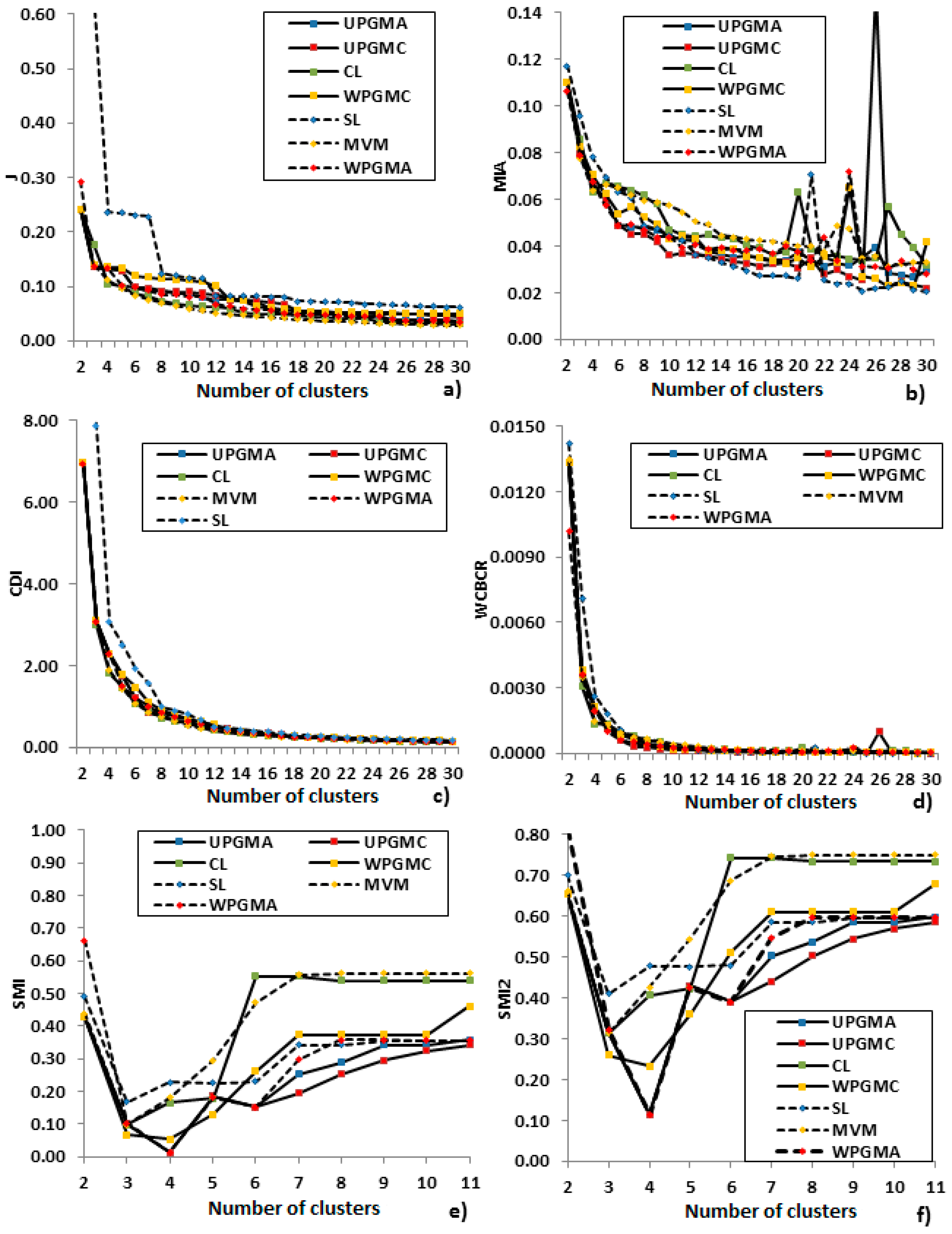
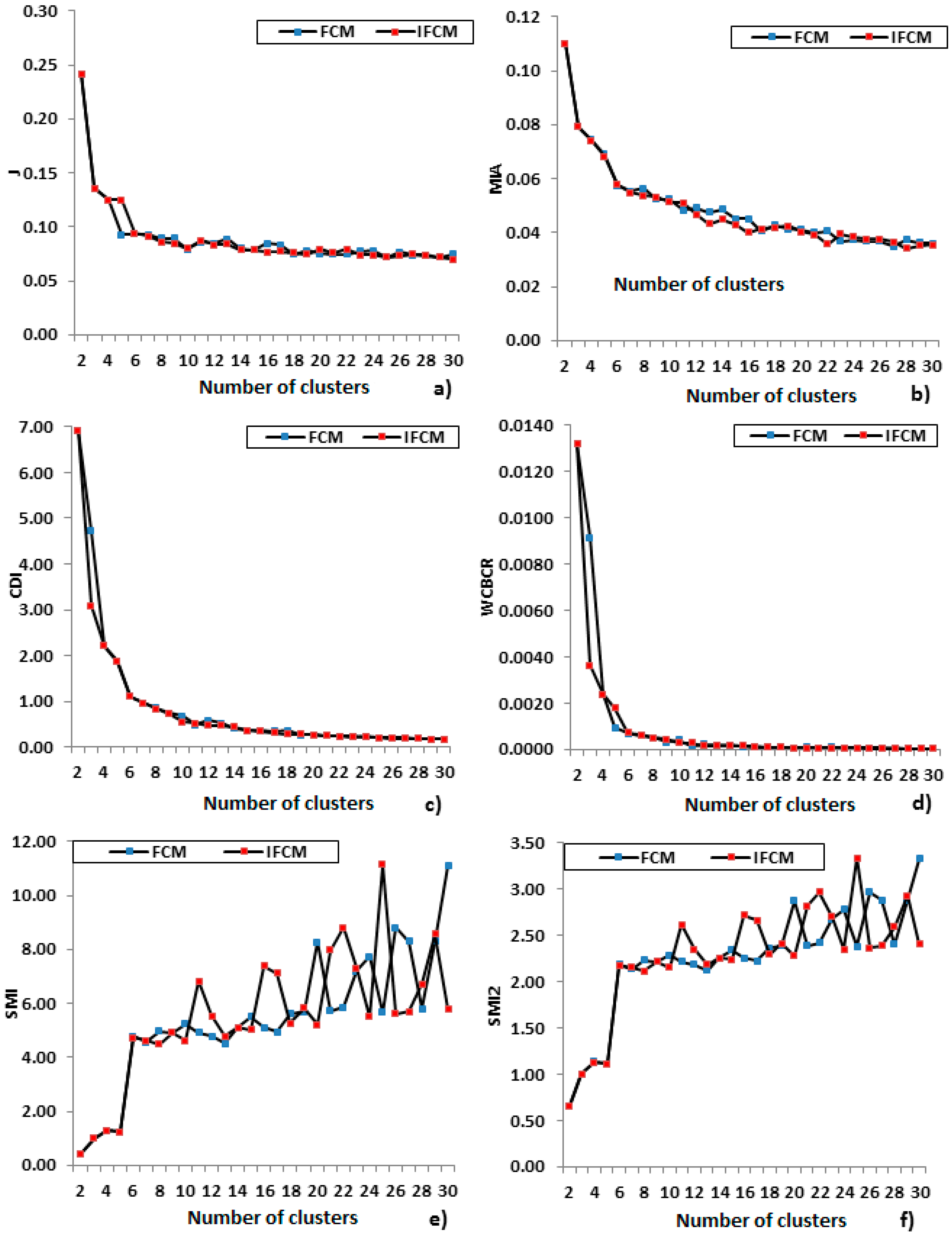
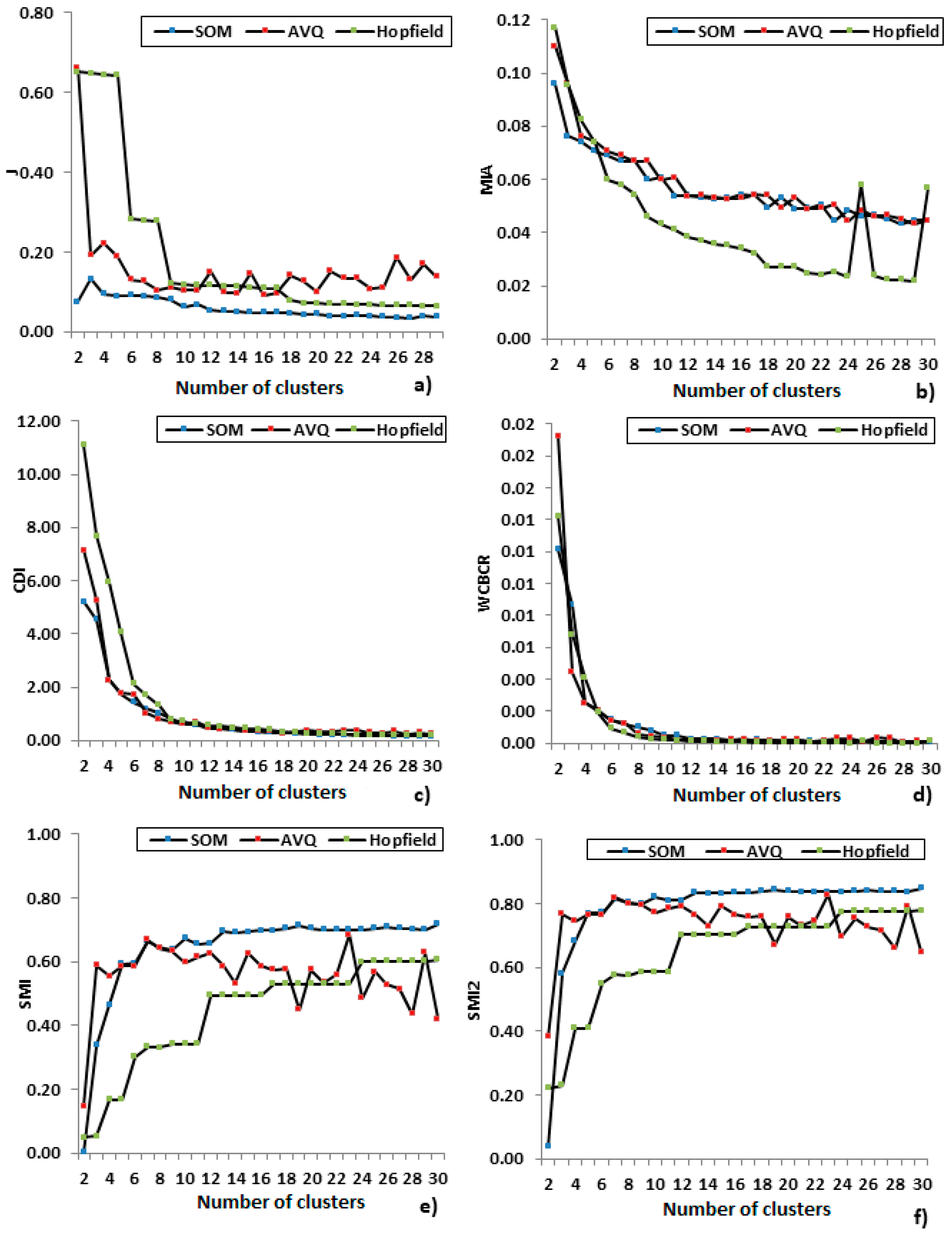
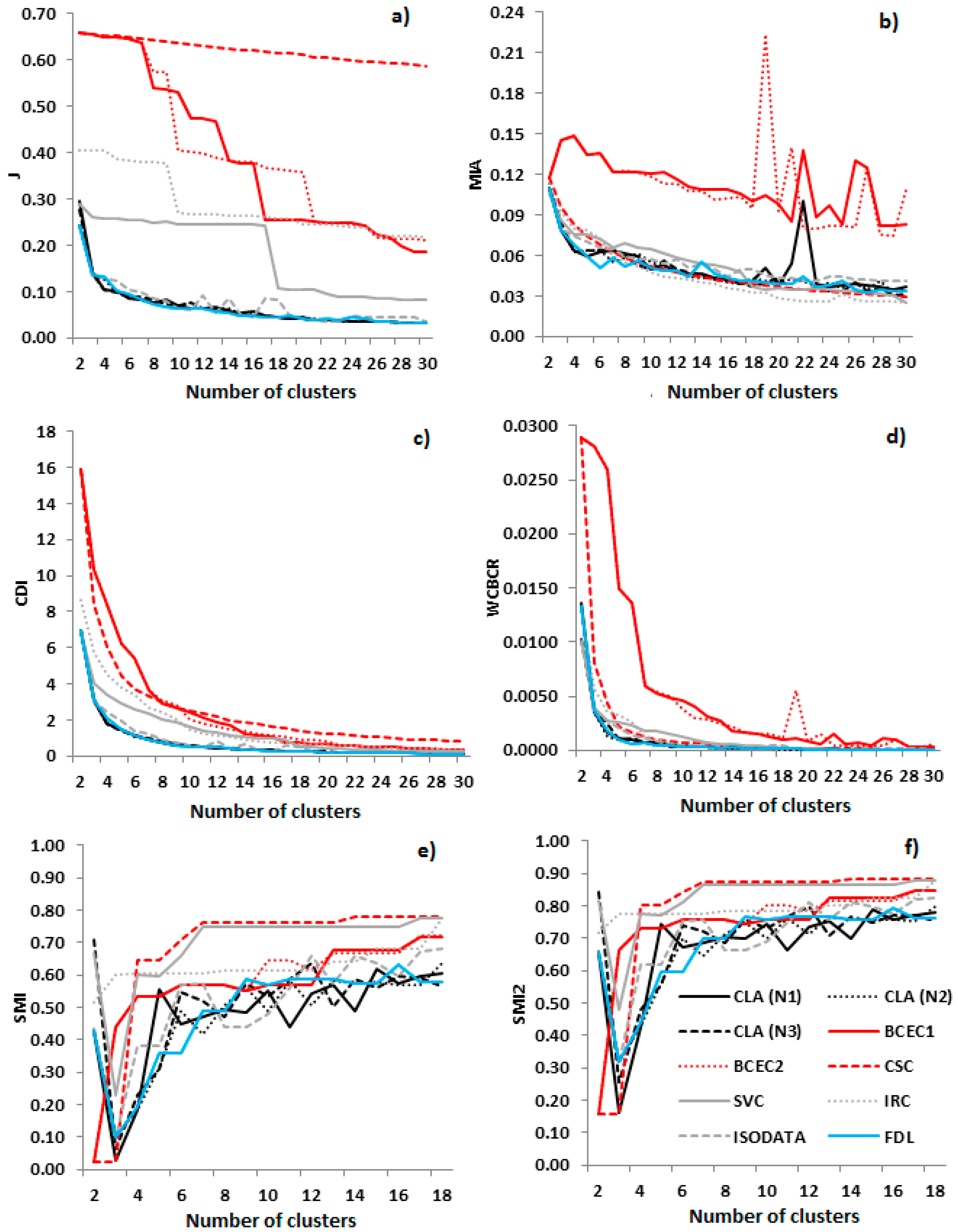
  • The Mean Square Error J, which refers to the sum of distances between the patterns and the clusters that belong to:
    J = 1 N n = 1 y n S k N d e u c l 2 ( y n , c k )
  • The Mean Index Adequacy (MIA), which refers to the average of the distances of the clusters:
    MIA = 1 K k = 1 K d e u c l 2 ( c k , S k )
  • The Clustering Dispersion Indicator (CDI), which refers to the ratio of the mean intra-set distance between the patterns in the same cluster and the inter-set distance between the clusters centroids:
    CDI = 1 K k = 1 K d e u c l 2 ( S k ) 1 2 K K = 1 K d e u c l 2 ( c k , C k )
  • The ratio of Within Cluster Sum of Squares to Between Cluster Variation (WCBCR), which corresponds to the ratio of the distance of each pattern from its cluster centroid and the sum of distances of the set Ck:
    WCBCR = k = 1 K n = 1 N d e u c l 2 ( c k , y n ) 1 s < t N d e u c l 2 ( y s , y t )
  • The Similarity Matrix Indicator (SMI), which takes into account the maximum of the centroid distances:
    SMI = max s > t { ( 1 1 ln [ d e u c l ( c s , c t ] ) 1 } : s , t = 1 , ... , K
  • The Similarity Matrix Indicator 2 (SMI2), which takes into account the root of maximum of the centroid distances:
    SMI 2 = max s > t { ( 1 1 ln [ d e u c l ( c s , c t ] ) 1 } : s , t = 1 , ... , K
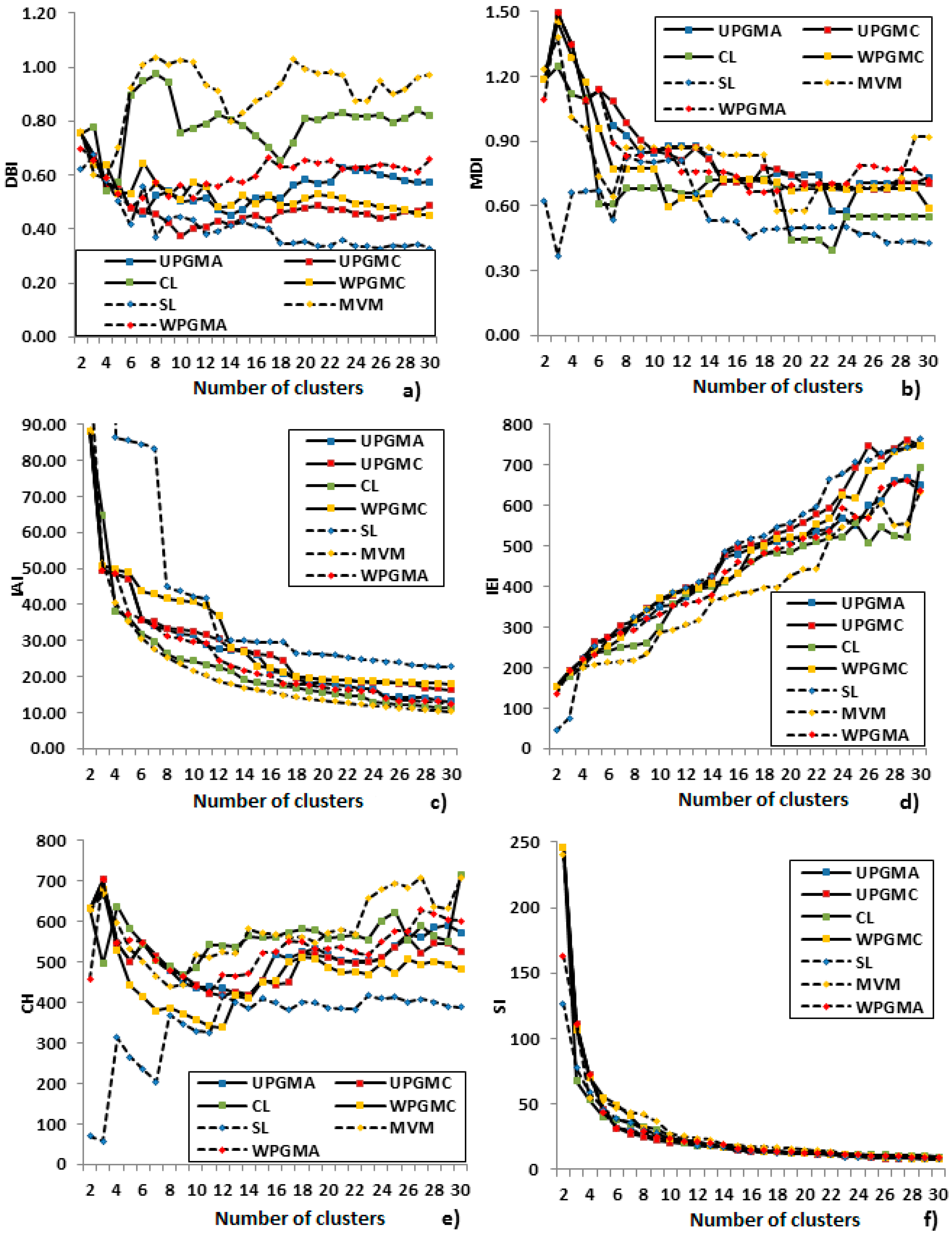
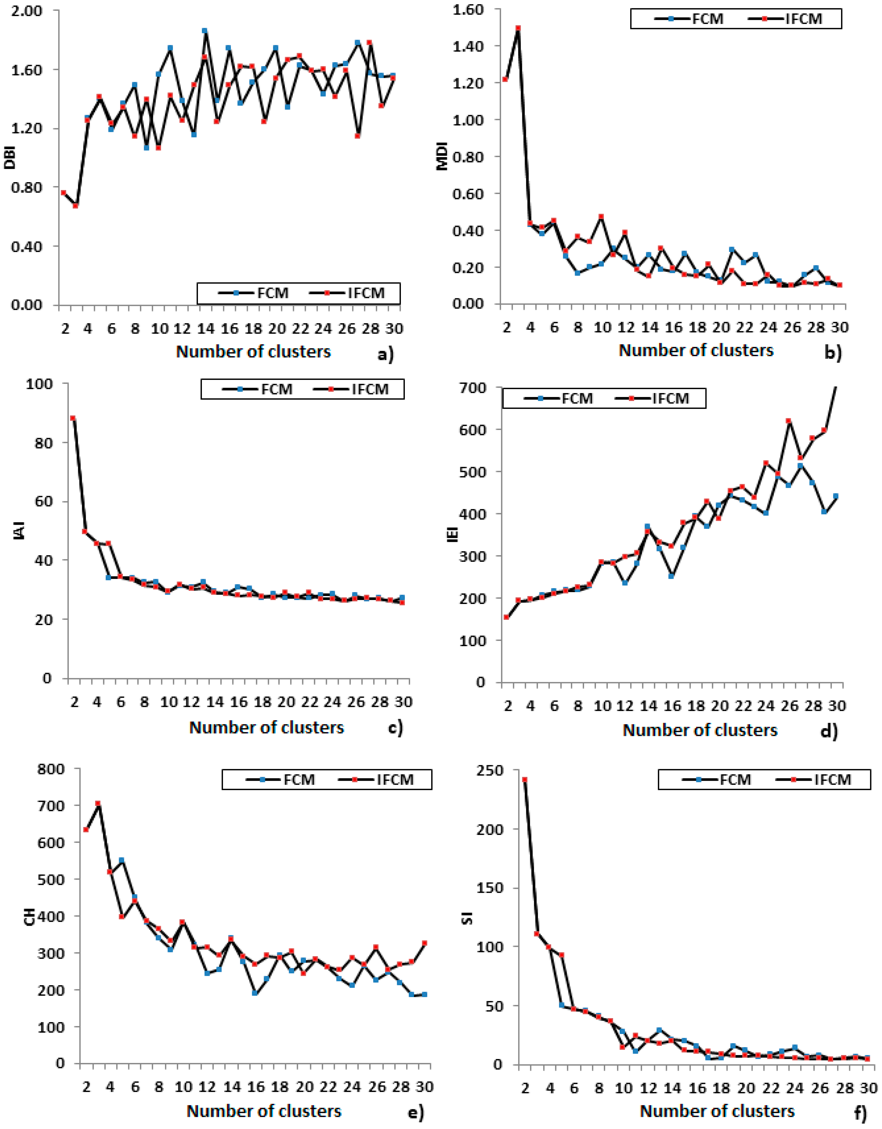
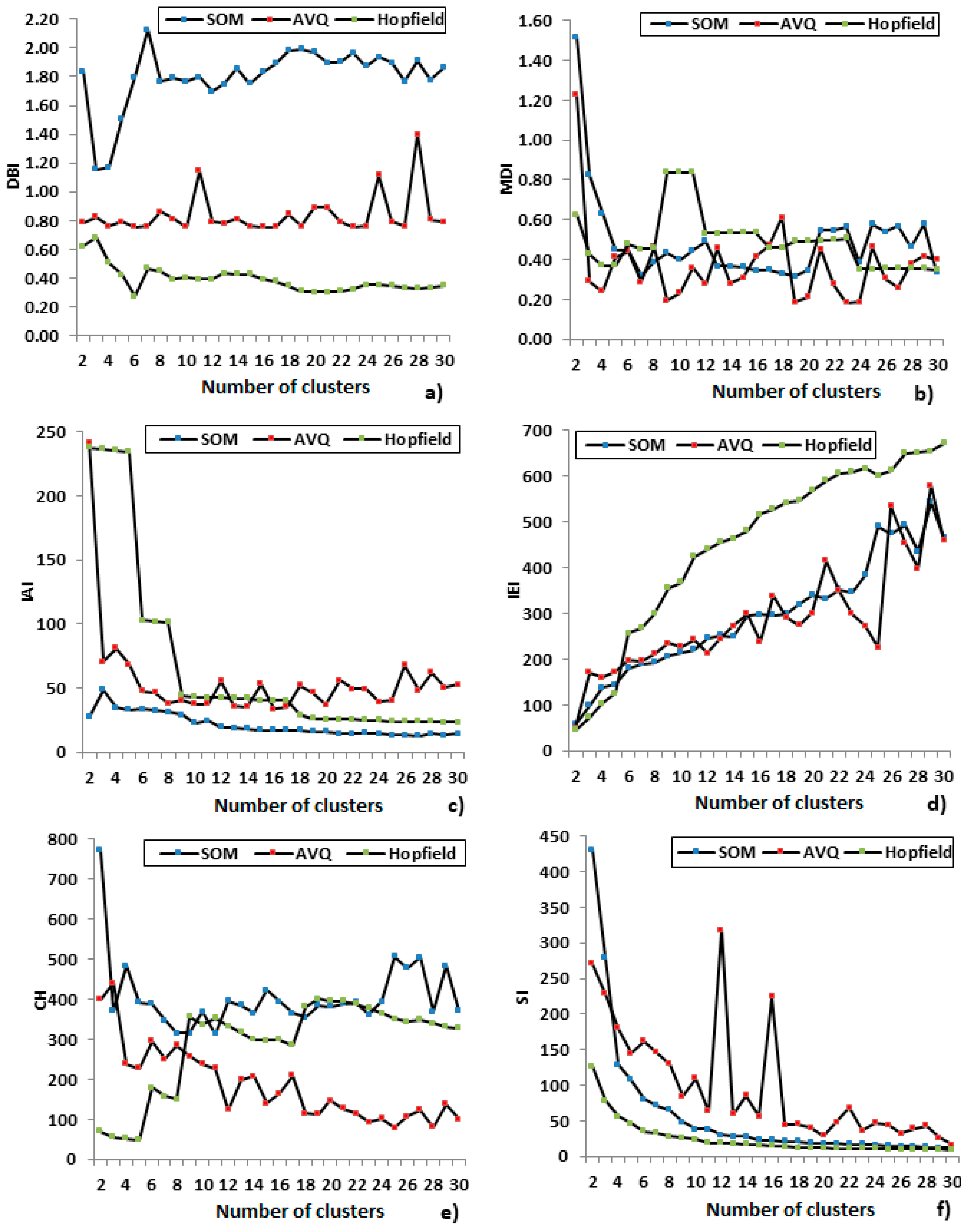
  • The Davies-Bouldin Index (DBI), which relates the mean distance of each cluster with the distance to the closest cluster:
    DBI = 1 K s , t = 1 K max s t { d ^ e u c l ( C s ) + d ^ e u c l ( C t ) d e u c l ( c s , c t ) }
  • The Modified Dunn Index (MDI), which takes into the minimum of the centroid distances:
    MDI = max 1 q K { d ^ ( C q ) } ( min s t { d ( c s , c t } ) 1
  • The Intra Cluster Index (IAI), which corresponds to the overall sum of the distances between patterns and centroids:
    IAI =    n = 1 N d e u c l 2 ( y n , c k )
  • The Inter Cluster Index (IEI), which corresponds to the sum of distances between the cluster centroids and the arithmetic mean:
    IEI = k = 1 K N k d e u c l ( c k , p )
    where p is the arithmetic mean of set X.
  • The Calinski index (CH) or Minimum Variance Criterion (VRC), which refers to the ratio of the separation among the different clusters and the separation within the same cluster:
    CH = N K K 1 IEI IAI
  • The Scatter Index (SI), which corresponds to the ratio of distances between the patterns and the arithmetic mean to the distances between the centroids and the arithmetic mean:
    SI = n = 1 N d e u c l 2 ( y n , p ) k = 1 K d e u c l 2 ( c k , p )
Some indices measure the compactness, others the separation or both of these cluster qualities.

3. TOPSIS

MCDA is applied to tasks where the decisions are taken in order to fulfil often contradictory criteria, e.g., minimum cost and minimum required time to deliver a project. The decision is a product of a systematic approach that partially or fully satisfies the conditions or limitations that each criterion places. The criteria may refer to technical and economic constrains, risk related factors, environmental restrictions and others. Basic tools of MCDA are the Analytical Hierarchical Process (AHP) and TOPSIS. During the last years, MCDA has witnessed a vast variety of applications [96]. In TOPSIS method, the solutions refer to the available alternative approaches for addressing the problem. In the present paper, the problem is the selection of the clustering algorithm that optimally clusters a given set of load data. The solutions are the clustering algorithms themselves and the criteria that need to be taken into account are “Criterion#1,” …, “Criterion#6.” Also, 2 solutions need to be defined, namely the “ideal” and the “anti-ideal.” The distances of each solution from the ideal and the anti-ideal ones are calculated. The selected solution should have minimum distance from the ideal and maximum distance from the anti-ideal solutions. Let A i , i = 1 , ... , r be the alternative solutions and z j , j = 1 , .. , p the criteria. The steps that construct the TOPSIS method are [19,97]:
Step#1.
Build the decision matrix D m a t r i x with i alternatives and j solutions:
    z 1    z 2    z j D m a t r i x = A 1 A 2 A i [ z 11 z 12 z 1 j z 21 z 22 z 2 j z i 1 z i 2 z i j ]
Step#2.
Construct the normalized D m a t r i x denoted as R with elements according to the following equation:
r i j = z i j i = 1 r z i j 2
Step#3.
Construct the weighted matrix R denoted as V according to:
V = [ v 11 v 12 v 1 j v 21 v 22 v 2 j v i 1 v i 2 v i j ]
where v i j = w i j r i j and w i j is the weight that solution A i is connected with criterion z j . It should be noted that the weights are fixed by the decision maker. The weights are user-centric and their values influence the results of the decision making. This fact is an inherent characteristic of TOPSIS method. Thus, TOPSIS offers a framework for the decision maker to include its expertise on a decision problem by setting the weights and reach into a solution that is in accordance to his/hers needs.
Step#4.
Calculate the ideal V + and the anti-ideal solution V according to:
V + = { ( max i v i j | j J ) , ( min i v i j | j J ) } V = { ( min i v i j | j J ) , ( max i v i j | j J ) }
where J and J are the positive and negative impact, respectively. More specifically, the ideal solution refers to is the maximum value for the positive impact and the minimum value for the negative impact in each column. Similarly, the anti-ideal solution, is the minimum and the maximum values for the positive and the negative impacts in each column, respectively.
Step#5.
Calculate the distances between each solution and the ideal and anti-ideal solutions:
S i + = i = 1 r ( v i j V + ) 2
S i = i = 1 r ( v i j V ) 2
Step#6.
Calculate the mean distance between each solution and anti-ideal solution as:
B i = S i S i + S i +
Step#7.
Sort the solutions according to the B i value.

4. Results

4.1. Algorithms Comparison

The data set under study correspond to a small industrial consumer and cover a period of a complete year. The dimension of patterns is D = 24, i.e., hourly measurements of active load are available. The data are normalized according to (1) and the set Y is obtained. Criterion#1 and Criterion#2 are indicators of algorithms’ complexity. Apart from the number of clusters that are needed to be obtained by an algorithm, other parameters may be needed such as number of iterations, threshold values and others. The fact that an algorithm demands many parameters leads to extra effort from the user to carefully select the parameters. These parameters may be extracted after experimentation or defined directly from the user, based on expertise and previous experience. Table 2, Table 3, Table 4, Table 5 and Table 6 present the parameters that partitional, hierarchical, fuzzy, neural-network based and other algorithms need prior to their execution, respectively. K-means requires 3 parameters, namely the maximum number of iterations, the initial centroids and the threshold of the objective function. The initial centroids are optional, i.e., the conventional edition of the algorithm selects automatically the centroids in a random manner. All partitional algorithms, apart from the number of clusters, require 3 parameters. It should be noted, that while all algorithms require 3 parameters, in many cases the required calibration time differs. This fact will be shown in Criterion#4. For example, while K-means and Modified K-means#1 need the same number of parameters, it is a more demanding effort to extract the optimal coefficients { a , b } compared to the initial centroids. According to Criterion#1 (i.e., minimum number of parameters that need to be specified), all partitional algorithms are similar in terms of complexity.
Moreover, hierarchical algorithms only need 1 parameter, the merging stopping criterion, which is indirectly related with the number of clusters. Regarding the fuzzy algorithms, the IFCM is more complex compared to the FCM. The IFCM is a hybrid algorithm that includes a clustering algorithm to extract the initial matrix U. According to [78], any clustering algorithm can be used for matrix initialization and thus, the input parameter requirements can be reduced if another algorithm is used. Hopfield ANN requires only the maximum number of iterations, a fact that makes it the most suitable neural-network based algorithm according to Criterion#1. The SOM needs many parameters, a fact that may lead to limitations in clustering applications with vast amount of metered load data where complexity and execution time are critical factors. The proper calibration of the SOM parameters, i.e., the dimension of the map, the type of learning function, the learning rate, the type of neighbourhood function, the number of epochs during training, etc. is a subject of detailed analysis. Regarding the algorithms of the rest category, ISODATA requires the most parameters. Between-Cluster Entropy-based Clustering #1 (BCEC1), Between-Cluster Entropy-based Clustering #2 (BCEC2) and Centroid Similarity-based Clustering (CSC) are hierarchical algorithms and thus only the merging stopping criterion is needed.
Criterion#2 is closely related with Criterion#1. It applies only if clusterings with different number of clusters are needed. Ideally, the execution of the algorithm for different number of clusters demands only the number of clusters itself. All the other parameters should remain constant and equal to their optimal values. The level of updating (i.e., periodically, prior to each execution, etc.) of the other parameters for different number of clusters, such as threshold values, number of iterations, etc., depends on the user preferences. The FDL, ISODATA, SVC and IRC do not require the number of clusters since this is indirectly defined from other parameters such as the parameter ρ in the FDL. Therefore, prior to each execution the parameters of the aforementioned algorithms should be re-defined. According to the paper’s experiments, FDL and ISODATA require a time demanding process to set the parameters in order for these algorithms to provide specific number of clusters. Table 7 shows the parameters that need to be updated.
Criterion#3 refers to the comparison via the validity indicators. The comparison per algorithm category is shown in Figure 1, Figure 2, Figure 3, Figure 4, Figure 5, Figure 6, Figure 7, Figure 8, Figure 9 and Figure 10. In the present paper, no information about the number of clusters is available, therefore this number should be determined by the validity indicator. The algorithms are executed for 2 to 30 clusters and for each number the score of the validity indicator is checked. Each algorithm is applied separately to the data set of the consumer. In the present paper, the maximum number of 30 is near the 10% of the patterns population, N = 365.
The superiority of an algorithm over the others is indicated when it leads, depending on the indicator, to lower or higher values in most of the clusters if not all. In some cases, an algorithm is more robust for certain number of clusters but it is surpassed by another for other number of clusters. Therefore, the general behaviour of an algorithm over a validity indicator should be examined.
The comparison of the partitional algorithms per validity indicator is illustrated in Figure 1 and Figure 2. Τhe number of pair of values of the coefficients { a , b } for the Modified K-means#1 and IWFA K-means are 1295. This means that 1295 clustering are generated from each algorithm. Only the one that leads to the lowest error is kept. In Figure 1 and Figure 2 the term “optimal” refers to the pair of values with lower error and the term “average” refer to the average value of the 1295 clusterings. For each validity indicator, different optimal pair of values is obtained. It can be noticed that there is no algorithm that wins the competition in all indicators, a finding that confirms the conclusions of the literature in algorithms comparison.
The graphs of J, MIA, CDI, WCBCR, SI and IAI display decreasing tendency while the number of clusters is increasing. The most efficient algorithm should lead to lower values of these indicators. This is also the case for DBI, SMI, SMI2 and MDI; these indicators display an unstable curve. In the IEI and CH the algorithm that wins the competition results in higher values. The J indicator expresses the sum of Euclidean distances among the patterns and the centroids. It is a measure of clusters’ compactness. The minCEntropy leads to lower errors followed by Modified Kmeans#1, K-medoids and K-means_B. Like the J indicator, MIA is a measure of compactness. Here the IWFA K-means is the most efficient followed by Modified Kmeans#2, minCEntropy and k-medoids.
The CDI and WCBCR both measure the compactness and separation. For the CDI, the ranking is minCEntropy, Modified K-means#2, K-medoids και Modified K-means#1. For the WCBCR, is Modified K-means#1, Modified K-means#2, ΙWFA K-means and minCEntropy. For the SMI and SMI2, the most robust are the Modified K-means#1, ΙWFA K-means, K-medoids and minCEntropy. The K-medoids and ΙWFA K-means win the competition according to DBI and MDI, respectively.
IAI is a modification of the J indicator; the same conclusions with J apply. Considering IEI, the algorithms ranking is ΙWFA K-means, Modified K-means#1, Modified K-means#2 and K-medoids. The CH indicator is the ratio of IAI and IEI. Therefore, it measures compactness and separation. Here the Modified K-means#1 is superior followed by the ΙWFA K-means, Modified K-means#1 and minCEntropy. Finally, SI measures the compactness of clusters. The algorithms ranking is the same with CH. After the comparison of the partitional algorithms, in general terms Modified K-means#1 and ΙWFA K-means are the most robust algorithms. Next, minCEntropy and K-medoids reach into the 3rd and 4th place in algorithms ranking.
Hierarchical agglomerative algorithms are characterized by the simplicity of their operation. The user should define the merging stopping criterion, which is actually the height that the dendrogram is cut. In respect to the algorithms of other categories, hierarchical clustering does not lead to clusters with zero number of members, i.e., empty clusters. Different executions always produce the same cluster. There is no need for a series of successive executions corresponding to different initializations.
The MVM is more efficient according to J and ΙΑΙ followed by CL, WPGMA and UPGMA. In MIA indicator the ranking is SL, UPGMC, UPGMA and WPGMC, while in CDI it is MVM, WPGMA, UPGMA and UPGMC. This comparison shows that MVM leads to lower errors in 6 indicators, namely at J, CDI, SMI, SMI2, MDI, IAI and CH. Next, the SL wins the competition according to ΜΙΑ, WCBCR, DBI, IEI and SI. Apart from these algorithms, robust performance is displayed by UPGMC and UPGMA.
Fuzzy algorithms are iterative and their operation present similarities with the K-means. The difference lies in the fact that they assign the patterns to all clusters. The fuzziness parameter defines the clusters’ composition. The increment of fuzziness parameter leads to more crisp clustering. After a parametric analysis, it is set to q = 2.70. The maximum number of iterations (i.e., epochs) of both the FCM and IFCM is set to 500. Also, the same number of iterations is set for the K-means that is used for the initialization of the IFCM. The IFCM results in lower errors according to J, MIA, CDI, WCBCR, DBI, MDI, IAI, IEI, CH and SI. In the cases of SMI and SMI2, the fuzzy algorithms have comparative performance.
Neural network-based algorithms need a proper parameter calibration analysis. For the AVQ, these are the initial learning rate η o and maximum number of iterations T max . The following ranges of values are considered: η o = { 0.05 , 0.01 , 0.15 , ... , 0.90 } and T max = { 100 , 200 , 300 , 400 , 500 } . After a set of experiments for the AVQ, the optimal values are drawn. For the J, MIA, CDI, WCBCR, SMI, SMI2, DBI, MDI, IAI, IEI, CH and SI indicators the optimal values are: {0.65, 100}, {0.90, 200}, {0.90, 100}, {0.90, 100}, {0.10, 300}, {0.60, 300}, {0.60, 100}, {0.65, 100}, {0.40, 100}, {0.10, 400} and {0.90, 400}, respectively.
The number of iterations for the Hopfield ANN is set to 50. According to results presented in Figure 7 and Figure 8, the Hopfield ANN leads to lower errors in MIA, WCBCR, DBI, IEI, SI, SMI and SMI2. In the cases of DBI and IEI, the difference among the algorithms is more visible. In the SI, for large number of clusters, SOM approaches the performance of Hopfield. In SMI and SMI2 for number of clusters above 18, the AVQ and Hopfield present similar behaviour. The SOM wins the competition in J and CDI. As for the MDI, special attention is needed to reach into safe conclusions for the algorithms comparison.
For CLA, 3 different normalization techniques are considered, namely N1, N2 and N3. The N1 performs a random selection of k patterns from the smallest hyper-rectangular that contains all vectors of Y. In the N2, a random selection of k patterns is held. Finally, in N3 the k most dissimilar patterns are selected. After a parametric analysis, the learning rates are set to η = 0.70 and η l = 0.00025 for all validity indicators. The maximum number of iterations is set to 500. The same number is set both for IRC and FDL.
For the SVC, the parameters are set to C = 1 and q = 1. For the ISODATA, the following values are selected: Threshold of number of patterns in a cluster is equal to 15, the threshold of distance for cluster merging equals 10 and the maximum number of iterations is also 10. From comparing the algorithms, it is shown that CLA leads to lower scores in J, IAI, SMI and SMI2. The most superior operation in CDI and CH is observed from FDL. In the case of the CDI, the difference between FDL and CLA is not large. In the cases of MIA and WCBCR, IRC is more efficient than the rest. Finally, CSC outmatches the rest in DBI and MDI and SVC in IEI and SI. From the comparison of the algorithms of the rest category, CLA is recommended.
Table 8 presents the algorithms ranking per validity indicator. The minCEntropy ranks 1st according to J, IAI and CDI. K-medoids ranks 1st in DBI and 4th in CDI. The Modified K-means#1 is present in 10 indices. According to Criterion#3, in general terms, it is the most efficient algorithm. IWFA K-means is the 2nd best. Also, minCEntropy ranks high in the lists. The results indicate that the partitional algorithms present better performance followed by hierarchical ones. Among the latter, SL is the most robust while MVM and UPGMC have satisfactory performance. No fuzzy and neural-network based algorithms are present. Among the algorithms of the rest category, IRC and CLA provide adequate clusterings.
Criterion#4 is important in applications with vast amount of data. Table 9 presents the execution time per algorithm as measured in 2.20 GHz Pentium® B960 Dual Core™ with 8 GB RAM system. The time refers only to the execution of the algorithm for 2 to 30 clusters excluding the calculation of the validity indicators value. Furthermore, the time of parametric analyses for proper parameter calibration is not included. The last column in the Table corresponds to the ratio of the required time of an algorithm to the required time of the K-means. All algorithms are executed considering their optimal parameters. It can be observed that hierarchical algorithms are the fastest. SOM and AVQ have considerably longer execution times, making these algorithms not appropriate for real-time applications. The required time for FDL and ISODATA cannot actually take part in the comparison since many different executions are needed by changing their parameters in order to provide clusterings with specific number of clusters.
Criterion#5 is application dependent. It refers to the potential of an algorithm to fit into the special requirements of an application. In the present paper, Criterion#5 considers the following attributes: Empty clusters generation and outlier detection. The results are presented in Table 10. The concept of “empty clusters” refers to the fact that an algorithm leads to lower number of clusters than the one it is requested. The concept “outlier detection” refers to the fact that an algorithm has the potential to track and isolate atypical patterns. Partitional algorithms do not result in empty clusters formation. However, they tend to produce clusters with almost similar number of members. On the contrary, hierarchical algorithms such as the SL and the CL algorithms can identify outliers. Therefore, hierarchical algorithms are suitable in data filtering, i.e., in cases that atypical data need to be excluded from the data set. Also, atypical data may refer to the load of holidays, working days close to holidays and other days with special attributes. The potential of tracking special days is suitable in load profiling applications.
Criterion#6 refers to software availability of the algorithms. Table 11 presents the software packages that include implementation of the algorithms. It can be noticed that most algorithms are available under commercial license or freely. In the cases of the K-means, K-medoids and hierarchical algorithms the Table presents the most common software. According to Table 11, there are lots of alternatives to implement these algorithms. The term “Matlab 3rd party code” refers to unofficial Matlab code freely provided by the authors. The term “In-house software” refers to code developed by the authors of the respective paper and is not officially distributed.

4.2. Algorithms Selection

The selection of the most proper algorithm for a given application is done using TOPSIS. The scope is to select an algorithm that maximizes the clustering benefit, i.e., the optimal segmentation of a given load data set. The initial phase of TOPSIS is the setting of the weights of each criterion. The sum of weights equals 1. The higher the weight of a criterion, the higher the importance this criterion has in the overall decision. While only clustering validity indicators are regarded in the load profiling literature, the weight of Criterion#3 is set with the higher value. Also, since smart metering installations and load data collections continue to increase, Criterion#4 has the next highest value. All the other criteria are equally valued. More specifically, let wCR(i) be the value of the ith criterion, I = 1, …, 6. The weights that are set to criteria are: wCR(1) = 0.10, wCR(2) = 0.10, wCR(3) = 0.40, wCR(4) = 0.20, wCR(5) = 0.10 and wCR(6) = 0.10. Let C#i, I = 1, …, 6 the indicator of criterion. Regarding the scores of the solution, the scale presented in Table 12 is taken into account. The decision matrix is shown in Table 13. Criterion#1, Criterion#2 and Criterion#4 need to be “minimized.” This means that an algorithm should score as less as possible. The ideal value is 1. This concept is reversed in Criterion#3, Criterion#5 and Criterion#6. In these cases, the ideal value is 9. In order to provide objective scores in Criterion#1, the actual number of parameters are set as scores. In Criterion#2, score “1” is matched to no requirements for parameter updating and score “2” is matched to 1 parameter. Additionally, scores “3” and “7” correspond to the actual numbers of parameters. Regarding Criterion#3, the following scores are taken under consideration: No presence in the ranking of Table 8 → 1, 1 presence in the ranking of Table 8 → 3, more than 1 presence in the ranking of Table 8 → 5, 1 presence and 1 higher rank in the ranking of Table 8 → 7 and more than 1 presence and more than 1 higher ranks in the ranking of Table 8 → 9. In Criterion#4, the actual execution durations in seconds are regarded. It should be noted that in TOPSIS, real numbers can also be considered as scores that do lie outside to the ordinary [1,2,…,9] scale. According to the results presented in Table 9, the FDL and ISODATA algorithm require large time that is considerable larger than the other algorithms. In order to express it in scale terms, they are considered to demand twice the time of the slowest algorithm, i.e., the AVQ. With reference to Criterion#5, the following scores are placed in {Empty clusters, Outlier tracking} pair: {Yes, No} → 1, {Yes, Yes} → 2, {No, No} → 3 and {No, Yes} → 4. Regarding Criterion#6, the “In-house software” is scored as “1” since in this case the algorithm is not available. All the other scores actually refer to real number of software packages that implement the algorithm. If the algorithm is available as a Matlab 3rd party code it scores 2.
The ideal solution is V + = [0.0056, 0.0104, 0.1606, 0.022, 0.030] and the anti-deal solution is V = [0.0398, 0.0729, 0.0178, 0.1175, 0.0055, 0.0033]. Table 14 presents the results of the application of the TOPSIS method. The last column of the matrix shows the ranking. The comparison of the algorithms indicate that SL is the most efficient followed by the K-medoids. In all criteria, the SL scores sufficiently. Also, the hierarchical algorithms UPGMA, UPGMC and MVM are highly ranked.
By comparing the algorithms’ categories, hierarchical algorithms are more suitable. The 2nd place belongs to partitional algorithms and the 3rd place to the algorithms of the rest category. Although Hopfield ANN ranks in the middle of the list, in general terms, the neural-network based algorithms is the category that ranks last. FDL and ISODATA are the least efficient algorithms. This is mainly due to the large time that is needed to extract a certain number of clusters. Therefore, it is recommended to select an algorithm that is directly fed with the number of clusters as an input parameter rather than defining the number of clusters through other parameters, e.g., distance threshold. According to Table 8, partitional algorithms lead to lowest errors than the rest. However, Modified K-means#1 and IWFA K-means#2 are complex in terms of required execution time. Overall, hierarchical clustering has 3 main advantages: Minimum input parameter requirements, speed and software availability.

5. Conclusions

Modern power system community has recognized the need to upgrade the role of the consumer in competitive energy market. The installation of smart metering is supported by the current legislative framework of European Union. The ideal case is that every consumer operates a smart meter. However, when the techno-economic barriers are present, alternative approaches should be considered to derive the typical demand patterns of the consumers. In many electricity networks, high-level consumer macro-categorization like residential, industrial and others is not robust. More detailed categorization is needed. The term “load profiling” refers to set of processes that lead to the characterization of the demand patterns of various consumers’ categories. Load profiling is a flexible tool that can aid in the formulation of the typical patterns for single consumers or group of consumers. The load curves are grouped together based on their similarity. Usually, no other parameters are needed apart from the load data. The importance of efficient load profiling is evident in a wide range of contemporary research topics like demand side management, tariff design, load forecasting and others.
Load profiling has gathered the attention of researchers in the recent years. This led to proposing many algorithms for clustering various load data sets. In the majority of the papers, the performance of the algorithms is tested only with quantitative criteria, namely the adequacy measures or clustering validity indicators. In spite of the large number of researches, no single study has provided a framework capable of indicating the benefits and limitations of the algorithms through a detailed comparison. In the present paper, a systematic procedure is proposed to rank the majority of the algorithms proposed in literature. The comparison includes 30 algorithms using 6 validation criteria. Apart from the validity indicators of the literature, the criteria involve factors that refer to the complexity of an algorithm and its availability. The main conclusions of the paper are summarized in the following:
  • Partitional algorithms are ranked 1st if only validity indicators are used. In 10 indicators, a partitional algorithm ranks 1st. The most robust partitional algorithm is Modified K-means#1. It ranks 1st in 3 indicators and 2nd in 5. The minCEntropy follows as it ranks 1st in 3 indicators also. No fuzzy and neural-network based algorithms are present in the lists of Table 8. From the algorithms of the rest category, IRC, CLA, SVC and BCEC2 are present. The CLA is the most robust algorithm from this category.
  • Computational time is an important factor. In this comparison, hierarchical clustering outclasses the other categories. SOM, AVQ, FDL and ISODATA are not recommended due to high time requirements.
  • ISODATA and SOM are not recommended in problems where low complexity in terms of input parameter requirements is crucial. In this case, hierarchical algorithms are preferred.
  • Software implementation availability is significant in cases of lack of programing skills, need for tested and verified codes or other factors. According to this criterion, hierarchical clustering, K-means, K-medoids and FCM are available in commercial and freely distributed packages.
The present paper can serve as a guide for further algorithms comparisons and testing. Potential expansions of the developed framework may include further criteria and MCDA methods for evaluation. Also, the analysis will be applied in other data sets.

Author Contributions

Ioannis P. Panapakidis performed the research and wrote the paper. Georgios C. Christoforidis revised the paper and set the objectives.

Conflicts of Interest

The authors declare no conflict of interest.

References

  1. Park, C.K.; Kim, H.J.; Kim, Y.S. A study of factors enhancing smart grid consumer engagement. Energy Pol. 2014, 72, 211–218. [Google Scholar] [CrossRef]
  2. Gangale, F.; Mengolini, A.; Onyeji, I. Consumer engagement: An insight from smart grid projects in Europe. Energy Pol. 2013, 60, 621–628. [Google Scholar] [CrossRef]
  3. Boisvert, R.N.; Cappers, P.A.; Neenan, B. The benefits of customer participation in wholesale electricity markets. Elect. J. 2002, 15, 41–51. [Google Scholar] [CrossRef]
  4. Grigoras, G.; Scarlatache, F. Knowlegde extraction from Smart Meters for consumer classification. In Proceedings of the 2014 International Conference and Exposition on Electrical and Power Engineering, Iasi, Romania, 16–18 October 2014; pp. 978–982. [Google Scholar]
  5. Uhrig, M.; Mueller, R.; Leibfried, T. Statistical consumer modelling based on smart meter measurement data. In Proceedings of the 2014 International Conference on Probabilistic Methods Applied to Power Systems, Durham, UK, 7–10 July 2014; pp. 1–6. [Google Scholar]
  6. Garpetun, L.; Nylén, P.O. Benefits from smart meter investments. In Proceedings of the 22nd International Conference and Exhibition on Electricity Distribution, Stockholm, Sweden, 10–13 June 2013; pp. 1–4. [Google Scholar]
  7. Depuru, S.S.S.R.; Wang, L.; Devabhaktuni, V. Smart meters for power grid: Challenges, issues, advantages and status. Renew. Sust. Energy Rev. 2011, 15, 2376–2742. [Google Scholar] [CrossRef]
  8. Al-Wakeel, A.; Wu, J.; Jenkins, N. k-means based load estimation of domestic smart meter measurements. Appl. Energy 2017, 194, 333–342. [Google Scholar] [CrossRef]
  9. Jardini, J.A.; Tahan, C.M.V.; Gouvea, M.R.; Ahn, S.U.; Figueiredo, F.M. Daily load profiles for residential, commercial and industrial low voltage consumers. IEEE Trans. Power Del. 2000, 15, 375–380. [Google Scholar] [CrossRef]
  10. Chang, R.F.; Lu, C.N. Load profiling and its applications in power market. In Proceedings of the 2003 IEEE Power Engineering Society General Meeting, Toronto, ON, Canada, 13–17 July 2003; pp. 974–978. [Google Scholar]
  11. Tsekouras, G.J.; Kotoulas, P.B.; Tsirekis, C.D.; Dialynas, E.N.; Hatziargyriou, N.D. A pattern recognition methodology for evaluation of load profiles and typical days of large electricity customers. Elect. Power Syst. Res. 2008, 78, 1494–1510. [Google Scholar] [CrossRef]
  12. Harris, C. Electricity Markets, Pricing, Structures and Economics; John Wiley&Sons Inc.: West Sussex, UK, 2006. [Google Scholar]
  13. Rathod, R.R.; Garg, R.D. Regional electricity consumption analysis for consumers using data mining techniques and consumer meter reading data. Int. J. Elect. Power Energy Syst. 2016, 78, 368–374. [Google Scholar] [CrossRef]
  14. Aghabozorgi, S.; Shirkhorshidi, A.S.; Wah, T.Y. Time-series clustering-A decade review. Inf. Sciences 2015, 53, 16–38. [Google Scholar] [CrossRef]
  15. Cornuéjols, A.; Wemmert, C.; Gançarski, P.; Bennani, Y. Collaborative clustering: Why, when, what and how. Inf. Sci. 2018, 39, 81–95. [Google Scholar] [CrossRef]
  16. Saxena, A.; Prasad, M.; Gupta, A.; Bharill, N.; Patel, O.P.; Tiwari, A.; Er, M.J.; Ding, W.; Lin, C.T. A review of clustering techniques and developments. Neurocomputing 2017, 167, 664–681. [Google Scholar] [CrossRef]
  17. Chicco, G. Overview and performance assessment of the clustering methods for electrical load pattern. Energy 2012, 42, 68–80. [Google Scholar] [CrossRef]
  18. Gerbec, D.; Gasperic, S.; Smon, I.; Gubina, F. Consumers’ load profile determination based on different classification methods. In Proceedings of the 2003 IEEE Power Engineering Society General Meeting, Toronto, ON, Canada, 3–17 July 2003; pp. 990–995. [Google Scholar]
  19. Hwang, C.L.; Yoon, K. Multiple Attribute Decision Making: Methods and Applications; Springer: New York, NY, USA, 1981. [Google Scholar]
  20. Union of the Electricity Industry (EUROELECTRIC). Metering, Load Profiles and Settlement in Deregulated Markets; Union of the Electricity Industry: Brussels, Belgium, 2000. [Google Scholar]
  21. The Pacific Gas and Electric Company (PG&E). Available online: Https://www.pge.com/ (accessed on 26 December 2017).
  22. Southern California Edison (SCE). Available online: Https://www.sce.com/ (accessed on 26 December 2017).
  23. Wang, Q.; Zhang, W.C.; Tang, Y.; Zhao, B.; Qiu, L.P.; Gao, X.; Shao, G.H.; Xiong, W.H.; Shi, K.Q. A new load survey method and its application in component based load modeling. In Proceedings of the 2010 International Conference on Power System Technology, Hangzhou, China, 24–28 October 2010; pp. 1–5. [Google Scholar]
  24. Zhang, J.; Yan, A.; Chen, Z.; Gao, K. Dynamic synthesis load modeling approach based on load survey and load curves analysis. In Proceedings of the 2008 Third International Conference on Electric Utility Deregulation and Restructuring and Power Technologies, Nanjing, China, 6–9 April 2008; pp. 1067–1071. [Google Scholar]
  25. Chen, C.S.; Hwang, J.C.; Huang, C.W. Application of load survey systems to proper tariff design. IEEE Trans. Power Syst. 1997, 12, 1746–1751. [Google Scholar] [CrossRef]
  26. Chen, C.S.; Hwang, J.C.; Tzeng, Y.M.; Huang, C.W.; Cho, M.Y. Determination of customer load characteristics by load survey system at Taipower. IEEE Trans. Power Del. 1996, 11, 1430–1436. [Google Scholar] [CrossRef]
  27. Tsekouras, G.J.; Hatziargyriou, N.D.; Dialynas, E.N. Two-stage pattern recognition of load curves for classification of electricity customers. IEEE Trans. Power Syst. 2007, 22, 1120–1128. [Google Scholar] [CrossRef]
  28. Panapakidis, I.P.; Christoforidis, G.C. Implementation of modified versions of the K-means algorithm in power load curves profiling. Sustain. Cities Soc. 2017, 35, 83–93. [Google Scholar] [CrossRef]
  29. Chicco, G.; Napoli, R.; Piglione, F. Comparisons among clustering techniques for electricity customer classification. IEEE Trans. Power Syst. 2006, 21, 933–940. [Google Scholar] [CrossRef]
  30. Rhodes, J.D.; Cole, W.J.; Upshaw, C.R.; Edgar, T.F.; Webber, M.E. Clustering analysis of residential electricity demand profiles. Appl. Energy 2014, 135, 461–471. [Google Scholar] [CrossRef]
  31. Benítez, I.; Quijano, A.; Díez, J.L.; Delgado, I. Dynamic clustering segmentation applied to load profiles of energy consumption from Spanish customers. Int. J. Elect. Power Energy Syst. 2014, 55, 437–448. [Google Scholar] [CrossRef]
  32. Kim, Y.I.; Shin, J.H.; Song, J.J.; Yang, I.K. Customer clustering and TDLP (Typical Daily Load Profile) generation using the clustering algorithm. In Proceedings of the IEEE T&D Asia Conference and Exposition, Seoul, Korea, 26–30 October 2009; pp. 1–4. [Google Scholar]
  33. Koolen, D.; Sadat-Razavi, N.; Ketter, W. Machine learning for identifying demand patterns of home energy management systems with dynamic electricity pricing. Appl. Sci. 2017, 7, 1160. [Google Scholar] [CrossRef]
  34. Jota, P.R.S.; Silva, V.R.B.; Jota, F.G. Building load management using cluster and statistical analyses. Int. J. Elect. Power Energy Syst. 2011, 33, 1498–1505. [Google Scholar] [CrossRef]
  35. Notaristefano, A.; Chicco, G.; Piglione, F. Data size reduction with symbolic aggregate approximation for electrical load pattern grouping. IET Gener. Trans. Distrib. 2013, 7, 108–117. [Google Scholar] [CrossRef]
  36. Zakaria, Z.; Lo, K.L.; Sohod, M.H. Application of fuzzy clustering to determine electricity consumers’ load profiles. In Proceedings of the First International Power and Energy Conference, Putra Jaya, Malaysia, 28–29 November 2006; pp. 99–103. [Google Scholar]
  37. Lo, K.L.; Zakaria, Z.; Sohod, M.H. Determination of consumers’ load profiles based on two-stage fuzzy C-means. In Proceedings of the 5th WSEAS International Conference on Power Systems and Electromagnetic Compatibility, Corfu, Greece, 23–25 August 2005; pp. 212–217. [Google Scholar]
  38. Binh, P.T.T.; Ha, N.H.; Tuan, T.C.; Khoa, L.D. Determination of representative load curve based on fuzzy K-means. In Proceedings of the 4th International Power Engineering and Optimization Conference, Shah Alam, Malaysia, 23–24 June 2010; pp. 281–286. [Google Scholar]
  39. Anuar, N.; Zakaria, Z. Determination of fuzziness parameter in load profiling via Fuzzy C-Means. In Proceedings of the 2011 IEEE Control and System Graduate Research Colloquium, Shah Alam, Malaysia, 27–28 June 2011; pp. 139–142. [Google Scholar]
  40. Prahastono, I.; King, D.J.; Ozveren, C.S.; Bradley, D. Electricity load profile classification using fuzzy C-means method. In Proceedings of the 43rd International Universities Power Engineering Conference, Padova, Italy, 1–4 September 2008; pp. 1–5. [Google Scholar]
  41. Iglesias, F.; Kastner, W. Analysis of similarity measures in times series clustering for the discovery of building energy patterns. Energies 2013, 6, 579–597. [Google Scholar] [CrossRef]
  42. Anuar, N.; Zakaria, Z. Electricity load profile determination by using Fuzzy C-Means and Probability Neural Network. Energy Proc. 2012, 14, 1861–1869. [Google Scholar] [CrossRef]
  43. Gerbec, D.; Gasperic, S.; Smon, I.; Gubina, F. Allocation of the load profiles to consumers using probabilistic neural networks. IEEE Trans. Power Syst. 2005, 20, 548–555. [Google Scholar] [CrossRef]
  44. Chang, R.F.; Lu, C.N. Load profile assignment of low voltage customers for power retail market applications. IEE Proc. Gener. Trans. Distrib. 2003, 150, 263–267. [Google Scholar] [CrossRef]
  45. Verdú, S.V.; García, M.O.; Franco, F.J.G.; Encinas, N.; Marín, A.G.; Molina, A.; Lázaro, E.G. Characterization and identification of electrical customers through the use of self-organizing maps and daily load parameters. In Proceedings of the 2004 IEEE PES Power Systems Conference and Exposition, New York, NY, USA, 10–13 October 2004; pp. 809–966. [Google Scholar]
  46. Verdu, S.V.; Garcia, M.O.; Senabre, C.; Marin, A.G.; Franco, F.J.G. Classification, filtering and identification of electrical customer load patterns through the use of self-organizing maps. IEEE Trans. Power Syst. 2006, 21, 1672–1682. [Google Scholar] [CrossRef]
  47. McLoughlin, F.; Duffy, A.; Conlon, M. Analysing domestic electricity smart metering data using self organising maps. In Proceedings of the 2012 CIRED Workshop on the Integration of Renewables into the Distribution Grid, Lisbon, Portugal, 29–30 May 2012; pp. 1–4. [Google Scholar]
  48. Chicco, G.; Scutariu, M.; Napoli, R.; Piglione, F.; Postolache, P.; Toader, C. A review of concepts and techniques for emergent customer categorization. In Proceedings of the Telmark Discussion Forum, London, UK, 2–4 September 2002; pp. 51–58. [Google Scholar]
  49. Valero, S.; Ortiz, M.; Senabre, C.; Alvarez, C.; Franco, F.J.G.; Gabaldon, A. Methods for customer and demand response policies selection in new electricity markets. IET Proc. Gener. Trans. Distrib. 2007, 1, 104–110. [Google Scholar] [CrossRef]
  50. Wang, Z.; Bian, S.; Liu, Y.; Liu, Z. The load characteristics classification and synthesis of substations in large area power grid. Int. J. Elect. Power Energy Syst. 2013, 48, 71–82. [Google Scholar] [CrossRef]
  51. Rodrigues, F.; Duarte, J.; Figueiredo, V.; Vale, Z.; Cordeiro, M. A comparative analysis of clustering algorithms applied to load profiling. Mach. Learn. Data Min. Pat. Recogn. Lect. Notes Comp. Sci. 2003, 2734, 73–85. [Google Scholar]
  52. Figueiredo, V.; Rodriguez, F.; Vale, Z.; Gouveia, J.B. An electricity energy consumer characterization framework based on data mining techniques. IEEE Trans. Power Syst. 2005, 20, 596–602. [Google Scholar] [CrossRef]
  53. Benabbas, F.; Khadir, M.T.; Fay, D.; Boughrira, A. Kohonen map combined to the K-means algorithm for the identification of day types of Algerian electricity load. In Proceedings of the 7th Computer Information Systems and Industrial Management Applications, Ostrava, Czech Republic, 26–28 June 2008; pp. 78–83. [Google Scholar]
  54. Räsänen, T.; Voukantsis, D.; Niska, H.; Karatzas, K.; Kolehmainen, M. Data-based method for creating electricity use load profiles using large amount of customer-specific hourly measured electricity use data. Appl. Energy 2010, 87, 3538–3545. [Google Scholar] [CrossRef]
  55. Park, S.; Ryu, S.; Choi, Y.; Kim, J.; Kim, H. Data-driven baseline estimation of residential buildings for demand response. Energies 2015, 8, 10239–10259. [Google Scholar] [CrossRef]
  56. Hernández, L.; Baladrón, C.; Aguiar, J.M.; Carro, B.; Sánchez-Esguevillas, A. Classification and clustering of electricity demand patterns in industrial parks. Energies 2012, 5, 5215–5228. [Google Scholar] [CrossRef]
  57. López, J.J.; Aguado, J.A.; Martín, F.; Munoz, F.; Rodríguez, A.; Ruiz, J.E. Electric customer classification using Hopfield recurrent ANN. In Proceedings of the 5th International Conference on European Electricity Market, Lisboa, Portugal, 28–30 May 2008; pp. 1–6. [Google Scholar]
  58. Chicco, G.; Napoli, R.; Postolache, P.; Scutariu, M.; Toader, C. Customer characterization options for improving the tariff offer. IEEE Trans. Power Syst. 2003, 18, 381–387. [Google Scholar] [CrossRef]
  59. Carpaneto, E.; Chicco, G.; Napoli, R.; Scutariu, M. Customer classification by means of harmonic representation of distinguishing features. In Proceedings of the 2003 IEEE Bologna Power Tech Conference, Bologna, Italy, 23–26 June 2003; pp. 1–7. [Google Scholar]
  60. Carpaneto, E.; Chicco, G.; Napoli, R.; Scutariu, M. Electricity customer classification using frequency–domain load pattern data. Int. J. Elect. Power Energy Syst. 2006, 28, 13–20. [Google Scholar] [CrossRef]
  61. Panapakidis, I.P.; Alexiadis, M.C.; Papagiannis, G.K. Application of competitive learning clustering in the load time series segmentation. In Proceedings of the 48th International Universities’ Power Engineering Conference, Dublin, Ireland, 2–5 September 2013; pp. 1–6. [Google Scholar]
  62. Mutanen, A.; Ruska, M.; Repo, S.; Järventausta, P. Customer classification and load profiling method for distribution systems. IEEE Trans. Power Del. 2011, 26, 1755–1763. [Google Scholar] [CrossRef]
  63. Chicco, G.; Napoli, R.; Piglione, F. Application of clustering algorithms and self organising maps to classify electricity customers. In Proceedings of the IEEE 2003 Power Tech Conference, Bologna, Italy, 23–26 June 2003; pp. 1–7. [Google Scholar]
  64. Gerbec, D.; Gasperic, S.; Smon, I.; Gubina, F. Determination and allocation of typical load profiles to the eligible consumers. In Proceedings of the 2003 IEEE Power Tech Conference, Bologna, Italy, 23–26 June 2003; pp. 1–5. [Google Scholar]
  65. Chicco, G.; Scutariu, M.; Napoli, R.; Piglione, F.; Postolache, P.; Toader, C. Application of clustering techniques to load pattern-based electricity customer classification. In Proceedings of the 18th International Conference on Electricity Distribution, Turin, Italy, 6–9 June 2005; pp. 1–5. [Google Scholar]
  66. Chicco, G.; Napoli, R.; Piglione, F.; Postolache, P.; Scutariu, M.; Toader, C. Emergent electricity customer classification. IEE Proc. Gener. Trans. Distrib. 2005, 152, 164–172. [Google Scholar] [CrossRef]
  67. Tsekouras, G.J.; Kanellos, F.D.; Kontargyri, V.T.; Karanasiou, I.S.; Salis, A.D.; Mastorakis, N.E. A new classification pattern recognition methodology for power system typical load profiles. WSEAS Trans. Circ. Syst. 2008, 7, 1090–1104. [Google Scholar]
  68. Kohan, N.M.; Moghaddam, M.P.; Bidaki, S.M.; Yousefi, G.R. Comparison of modified K-means and hierarchical algorithms in customers load curves clustering for designing suitable tariffs in electricity market. In Proceedings of the 43rd International Universities Power Engineering Conference, Padova, Italy, 1–4 September 2008; pp. 1–5. [Google Scholar]
  69. Kohan, N.M.; Moghaddam, M.P.; Bidaki, S.M. Evaluating performance of WFA k-means and Modified Follow the Leader methods for clustering load curves. In Proceedings of the IEEE 2009 Power Systems Conference and Exposition, Seattle, WA, USA, 15–18 March 2009; pp. 1–5. [Google Scholar]
  70. Kohan, N.M.; Moghaddam, M.P.; Sheikh-El-Eslami, M.K.; Bidaki, S.M. Improving WFA k-means technique for demand response programs applications. In Proceedings of the IEEE 2009 Power & Energy Society General Meeting, Calgary, AB, Canada, 26–30 July 2009; pp. 1–5. [Google Scholar]
  71. Bidoki, S.M.; Kohan, N.M.; Sadreddini, M.H.; Zolghadri Jahromi, M.; Moghaddam, M.P. Evaluating different clustering techniques for electricity customer classification. In Proceedings of the 2010 IEEE PES Transmission and Distribution Conference and Exposition, New Orleans, LA, USA, 19–22 April 2010; pp. 1–5. [Google Scholar]
  72. Bidoki, S.M.; Kohan, N.M.; Gerami, S. Comparison of several clustering methods in the case of electrical load curves classification. In Proceedings of the 16th Conference on Electrical Power Distribution Networks, Bandar Abbas, Iran, 19–20 April 2011; pp. 1–7. [Google Scholar]
  73. López, J.J.; Aguado, J.A.; Martín, F.; Munoz, F.; Rodríguez, A.; Ruiz, J.E. Hopfield–K-means clustering algorithm: A proposal for the segmentation of electricity customers. Electr. Power Syst. Res. 2011, 81, 716–722. [Google Scholar] [CrossRef]
  74. Chicco, G.; Akilimali, J.S. Renyi entropy-based classification of daily electrical load patterns. IET Gener. Trans. Distrib. 2010, 4, 736–745. [Google Scholar] [CrossRef]
  75. Chicco, G.; Ilie, I.S. Support vector clustering of electrical load pattern data. IEEE Trans. Power Syst. 2009, 24, 1619–1628. [Google Scholar] [CrossRef]
  76. Marques, D.Z.; de Almeida, K.A.; de Deus, A.M.; da Silva Paulo, A.R.G.; da Silva Lima, W. A comparative analysis of neural and fuzzy cluster techniques applied to the characterization of electric load in substations. In Proceedings of the 2004 IEEE/PES Transmission and Distribution Conference and Exposition Latin America, Sao Paulo, Brazil, 8–11 November 2004; pp. 908–913. [Google Scholar]
  77. Panapakidis, I.P.; Alexiadis, M.C.; Papagiannis, G.K. Load profiling in the deregulated electricity markets: A review of the applications. In Proceedings of the 9th International Conference on the European Energy Market, Florence, Italy, 10–12 May 2012; pp. 1–6. [Google Scholar]
  78. Panapakidis, I.; Asimopoulos, N.; Dagoumas, A.; Christoforidis, G.C. An improved Fuzzy C-Means algorithm for the implementation of demand side management measures. Energies 2017, 10, 1407. [Google Scholar] [CrossRef]
  79. Panapakidis, I.P.; Alexiadis, M.C.; Papagiannis, G. Evaluation of the performance of clustering algorithms for a high voltage industrial consumer. Eng. Appl. Art. Intell. 2015, 38, 1–13. [Google Scholar] [CrossRef]
  80. Batrinu, F.; Chicco, G.; Napoli, R.; Piglione, F.; Postolache, P.; Scutariu, M.; Toader, C. Efficient iterative refinement clustering for electricity customer classification. In Proceedings of the 2005 IEEE Russia Power Tech Conference, St. Petersburg, Russia, 27–30 June 2005; pp. 1–7. [Google Scholar]
  81. McLoughlin, F.; Duffy, A.; Conlon, M. A clustering approach to domestic electricity load profile characterisation using smart metering data. Appl. Energy 2015, 141, 190–199. [Google Scholar] [CrossRef]
  82. Kang, J.; Lee, J.H. Electricity customer clustering following experts’ principle for demand response applications. Energies 2015, 8, 12242–12265. [Google Scholar] [CrossRef]
  83. Apetrei, D.; Silvas, I.; Albu, M.; Postolache, P. Consideration on relationship between load dispatching and load profile clustering. In Proceedings of the 10th International Conference on Environment and Electrical Engineering, Rome, Italy, 8–11 May 2011; pp. 1–4. [Google Scholar]
  84. Mori, H.; Yuihara, A. Deterministic annealing clustering for ANN-based short-term load forecasting. IEEE Trans. Power Syst. 2011, 16, 545–551. [Google Scholar] [CrossRef]
  85. Mahmoudi-Kohan, N.; Parsa Moghaddam, M.; Sheikh-El-Eslami, M.K.; Shayesteh, E. A three-stage strategy for optimal price offering by a retailer based on clustering techniques. Int. J. Electr. Power Energy Syst. 2010, 32, 1135–1142. [Google Scholar] [CrossRef]
  86. Li, Y.; Guo, P.; Li, X. Short-term load forecasting based on the analysis of user electricity behaviour. Algorithms 2016, 9, 80. [Google Scholar] [CrossRef]
  87. Gao, Y.; Sun, Y.; Wang, X.; Chen, F.; Ehsan, A.; Li, H.; Li, H. Multi-objective optimized aggregation of demand side resources based on a self-organizing map clustering algorithm considering a multi-scenario technique. Energies 2017, 10, 144. [Google Scholar] [CrossRef]
  88. Li, Y.H.; Wang, J.X. Flexible transmission network expansion planning considering uncertain renewable generation and load demand based on hybrid clustering analysis. Appl. Sci. 2016, 6, 3. [Google Scholar] [CrossRef]
  89. Qiu, X.; Zhang, L.; Ren, Y.; Suganthan, P.N.; Amaratunga, G. Ensemble deep learning for regression and time series forecasting. In Proceedings of the 2014 IEEE Symposium on Computational Intelligence in Ensemble Learning (CIEL), Orlando, FL, USA, 9–12 December 2014; pp. 1–6. [Google Scholar]
  90. Qiu, X.; Zhang, L.; Suganthan, P.N.; Amaratunga, G.A.J. Oblique random forest ensemble via Least Square Estimation for time series forecasting. Inf. Sci. 2017, 420, 249–262. [Google Scholar] [CrossRef]
  91. Steinley, D. K-means clustering: A half-century synthesis. Br. J. Math. Stat. Psychol. 2006, 59, 1–34. [Google Scholar] [CrossRef] [PubMed]
  92. Xu, R.; Wunsch, D. Clustering, 1st ed.; John Wiley & Sons Inc.: Hoboken, NJ, USA, 2006. [Google Scholar]
  93. De Oliveria, J.V.; Pedrycz, W. Advances in Fuzzy Clustering and Its Applications, 1st ed.; John Wiley & Sons: Chichester, UK, 2007; pp. 373–424. [Google Scholar]
  94. Grossberg, S. Adaptive pattern classification and universal recoding: I. Parallel development and coding of neural feature detectors. Biolog. Cyber. 1976, 23, 121–134. [Google Scholar] [CrossRef]
  95. Kohonen, T. Self-Organisation and Associative Memory, 3rd ed.; Springer: Berlin, Germany, 1989. [Google Scholar]
  96. Zyoud, S.H.; Fuchs-Hanusch, D. A bibliometric-based survey on AHP and TOPSIS techniques. Exp. Syst. Appl. 2017, 78, 158–181. [Google Scholar] [CrossRef]
  97. Aalami, H.A.; Parsa Moghaddam, M.; Yousefi, G.R. Modeling and prioritizing demand response programs in power markets. Elec. Power Syst. Res. 2010, 80, 426–435. [Google Scholar] [CrossRef]
  98. MathWorks®. Available online: https://www.mathworks.com (accessed on 26 December 2017).
  99. WOLFRAM. Available online: https://www.wolfram.com (accessed on 26 December 2017).
  100. The R Project for Statistical Computing. Available online: https://www.r-project.org (accessed on 26 December 2017).
  101. WEKA The University of Waikato. Available online: https://www.cs.waikato.ac.nz/ml/weka (accessed on 26 December 2017).
  102. Microsoft. Available online: https://www.visualstudio.com (accessed on 26 December 2017).
  103. Python™. Available online: https://www.python.org (accessed on 26 December 2017).
Figure 1. Comparison of the partitional algorithms using: (a) J, (b) MIA, (c) CDI, (d) WCBCR, (e) SMI, (f) SMI2.
Applsci 08 00237 g001
Figure 2. Comparison of the partitional algorithms using: (a) DBI, (b) MDI, (c) IAI, (d) IEI, (e) CH, (f) SI.
Applsci 08 00237 g002
Figure 3. Comparison of the hierarchical algorithms using: (a) J, (b) MIA, (c) CDI, (d) WCBCR, (e) SMI, (f) SMI2.
Applsci 08 00237 g003
Figure 4. Comparison of the hierarchical algorithms using: (a) DBI, (b) MDI, (c) IAI, (d) IEI, (e) CH, (f) SI.
Applsci 08 00237 g004
Figure 5. Comparison of the fuzzy algorithms using: (a) J, (b) MIA, (c) CDI, (d) WCBCR, (e) SMI, (f) SMI2.
Applsci 08 00237 g005
Figure 6. Comparison of the fuzzy algorithms using: (a) DBI, (b) MDI, (c) IAI, (d) IEI, (e) CH, (f) SI.
Applsci 08 00237 g006
Figure 7. Comparison of the neural network-based algorithms using: (a) J, (b) MIA, (c) CDI, (d) WCBCR, (e) SMI, (f) SMI2.
Applsci 08 00237 g007
Figure 8. Comparison of the neural network-based algorithms using: (a) DBI, (b) MDI, (c) IAI, (d) IEI, (e) CH, (f) SI.
Applsci 08 00237 g008
Figure 9. Comparison of the rest algorithms using: (a) J, (b) MIA, (c) CDI, (d) WCBCR, (e) SMI, (f) SMI2.
Applsci 08 00237 g009
Figure 10. Comparison of the rest algorithms using: (a) DBI, (b) MDI, (c) IAI, (d) IEI, (e) CH, (f) SI.
Applsci 08 00237 g010
Table 1. Coefficients of the hierarchical agglomerative algorithms.
Algorithm a i a j β γ
Single Linkage (SL)0.500.5000.50
Complete Linkage (CL)0.500.5000.50
Unweighted Pair Group Method Average (UPGMA)0.50 N j N i + N j 00
Weighted Pair Group Method Average (WPGMA)0.500.5000
Weighted Pair Group Method Centroid (WPGMC)0.500.50−0.250
Unweighted Pair Group Method Centroid (UPGMC) N i N i + N j N j N i + N j N i N j ( N i + N j ) 2 0
Minimum Variance Method (MVM) or the Ward’s method N i + N l N i + N j + N l N j + N l N i + N j + N l N j N i + N j + N l 0
Table 2. Parameters of the partitional algorithms.
AlgorithmParameters for Determination
K-means1. Maximum number of iterations
2. Initial centroids (optional)
3. Minimum objective function improvement threshold
Modified K-means#11. Maximum number of iterations
2. Optimal coefficients { a , b }
3. Minimum objective function improvement threshold
Modified K-means#21. Maximum number of iterations
2. Coefficients { a i , b i }
3. Minimum objective function improvement threshold
WFA K-means1. Maximum number of iterations
2. Initial centroids (optional)
3. Minimum objective function improvement threshold
IWFA K-means1. Maximum number of iterations
2. Optimal coefficients { a , b }
3. Minimum objective function improvement threshold
Hopfield K-means1. Maximum number of iterations for Hopfield ANN
2. Maximum number of iterations K-means
3. Minimum objective function improvement threshold
minCEntropy1. Maximum number of iterations
2. Parameter σ
3. Minimum objective function improvement threshold
K-means_A1. Maximum number of iterations
2.Minimum objective function improvement threshold
K-means_B1. Maximum number of iterations
2.Minimum objective function improvement threshold
K-medoids1. Maximum number of iterations
2. Initial centroids (optional)
3.Minimum objective function improvement threshold
Table 3. Parameters of the hierarchical algorithms.
AlgorithmParameters for Determination
SLMerging stopping criterion
CLMerging stopping criterion
UPGMAMerging stopping criterion
WPGMAMerging stopping criterion
WPGMCMerging stopping criterion
UPGMCMerging stopping criterion
MVMMerging stopping criterion
Table 4. Parameters of the fuzzy algorithms.
AlgorithmParameters for Determination
FCM1. Maximum number of iterations
2. Initial centroids (optional)
3. Minimum objective function improvement
4. Fuzzy parameter q
5. Initial values of matrix U
ΙFCM1. Maximum number of iterations for the K-means
2. Maximum number of iterations for the FCM
3. Initial centroids for the K-means (optional)
4.Minimum objective function improvement threshold for the K-means
5.Minimum objective function improvement threshold for the FCM
6. Fuzzy parameter q
Table 5. Parameters of the neural network-based algorithms.
AlgorithmParameters for Determination
AVQ1. Maximum number of iterations
2. Constant parameter of the learning rate
SOM1. Dimension (1D or 2D)
2. Map shape
3. Map size
4. Weights initialization
5. Learning method
6.Learning function (type, initial learning rate, training epochs)
7.Neighborhood function (type, initial neighbourhood radius)
HopfieldMaximum number of iterations
Table 6. Parameters of the rest algorithms.
AlgorithmParameters for Determination
FDL1. Maximum number of iterations
2. Initial centroids (optional)
3. Parameter ρ
ISODATA1. Maximum number of clusters
2. Maximum number of clusters for merging
3. Maximum number of iterations
4. Threshold of number of patterns in a cluster
5. Threshold of distance for cluster merging
6. Threshold of standard deviation for cluster split
7. Minimum distance between patterns and centroid
BCEC1Merging stopping criterion
BCEC2Merging stopping criterion
CSCMerging stopping criterion
SVC1.Parameter that controls the number of outliers
2. Scale parameter of the Gaussian kernel
3. Minimum distance
4. Cluster formation threshold
IRC1. Maximum number of iterations
2. Parameter ρ
CLA1. Maximum number of iterations
2. Initial centroids (optional)
3. Constant term of learning rate (winner neuron)
4. Constant term of learning rate (rest neurons)
Table 7. Parameters updating requirements.
AlgorithmParameter
K-means-
Modified K-means#1-
Modified K-means#2-
WFA K-means-
IWFA K-means-
Hopfield K-means-
minCEntropy-
Κ-means_A-
Κ-means_B-
K-medoids-
SL-
CL-
UPGMA-
WPGMA-
WPGMC-
UPGMC-
MVM-
FCM-
IFCM-
SOM-
AVQ-
Hopfield-
FDLParameter ρ
CLA-
IRCParameter ρ
BCEC1-
BCEC2-
CSC-
SVC1. Minimum distance
2. Cluster formation threshold
ISODATA1. Maximum number of clusters
2. Maximum number of clusters for merging
3. Maximum number of iterations
4. Threshold of number of patterns in a cluster
5. Threshold of distance for cluster merging
6. Threshold of standard deviation for cluster split
7.Minimum distance between patterns and centroid
Table 8. Algorithms ranking per validity indicator.
Validity IndicatorAlgorithms’ RankingValidity IndicatorAlgorithms’ Ranking
J1. minCEntropy
2. Modified K-means#1
3. MVM
4. K-means_A
MDI1. IRC
2. IWFA K-means
3. Modified K-means#1
4. BCEC2
MIA1. SL
2. IWFA K-means
3. UPGMC
4. UPGMA
IAI1. minCEntropy
2. Modified K-means#1
3. MVM
4. K-means_A
CDI1. minCEntropy
2. Modified K-means#1
3. MVM
4. K-medoids
IEI1. IWFA K-means
2. Modified K-means#1
3. SVC
4. IRC
WCBCR1. SL
2. UPGMC
3. Modified K-means#1
4. UPGMA
CH1. Modified K-means#1
2. IWFA K-means
3. minCEntropy
4. MVM
SMI1. Modified K-means#1
2. CLA (N3)
3. MVM
4. CLA (N2)
SI1. IWFA K-means
2. Modified K-means#1
3. SL
4. UPGMC
SMI21. Modified K-means#1
2. CLA (N3)
3. MVM
4. CLA (N2)
DBI1. K-medoids
2. SL
3. UPGMC
4. UPGMA
Table 9. Required execution time per algorithm.
AlgorithmExecution Time (s)Ratio
K-means8.311
Modified K-means# 1978.81117.78
Modified K-means#2 215.931.91
WFA K-means8.441.01
IWFA K-means 1713.8085.89
Hopfield K-means49.535.96
minCEntropy691.7383.24
Κ-means_A8.270.99
K-means_B8.160.98
K-medoids9.221.10
SL3.590.43
CL3.690.44
UPGMA3.670.44
WPGMA3.680.44
WPGMC3.710.44
UPGMC3.730.44
MVM3.700.44
FCM10.911.31
IFCM13.321.60
SOM (1D)1148138.14
AVQ 31244.70149.78
Hopfield44.695.37
FDL>>0>>1
CLA 4848.97102.16
IRC6.410.77
BCEC1 56.830.82
BCEC2 56.610.79
CSC 56.530.78
SVC27.543.31
ISODATA>>0>>1
1 The calculation of the optimal pair of values { a , b } is not included. 2 The calculation of the pair of values { a i , b i } is not included. 3 The optimal parameters of the WCBCR are regarded. 4 The N1 normalization is regarded. 5 The calculation of the entropy matrix is not included.
Table 10. Algorithms comparison in terms of empty clusters formation and outliers tracking.
AlgorithmEmpty ClustersOutliers Tracking
K-meansNoNo
Modified K-means#1NoNo
Modified K-means#2NoNo
WFA K-meansNoNo
IWFA K-meansNoNo
Hopfield K-meansNoNo
minCEntropyNoNo
Κ-means_ANoNo
K-means_BNoNo
K-medoidsNoNo
SLNoYes
CLNoYes
UPGMANoYes
WPGMANoYes
WPGMCNoYes
UPGMCNoYes
MVMNoYes
FCMYesNo
IFCMYesNo
SOMNoNo
AVQYesNo
HopfieldNoNo
FDLNoYes
CLAYesNo
IRCNoYes
BCEC1NoYes
BCEC2NoYes
CSCNoYes
SVCNoYes
ISODATAYesNo
Table 11. Software availability per algorithm [98,99,100,101,102,103].
AlgorithmAvailability
K-means1. Matlab
2. Mathematica
3. SPSS
4. SAS
5. R
6. Weka
7. C++/C#
8. Python
9. Matlab 3rd party code
Modified K-means#1In-house software
Modified K-means#2In-house software
WFA K-meansIn-house software
IWFA K-meansIn-house software
Hopfield K-meansIn-house software
minCEntropyMatlab 3rd party code
Κ-means_AIn-house software
K-means_BIn-house software
K-medoids1. Matlab
2. Mathematica
3. SPSS
4. SAS
5. R
6. Weka
7. C++/C#
8. Python
9. Matlab 3rd party code
Hierarchical algorithms1. Matlab
2. Mathematica
3. SPSS
4. SAS
5. R
6. Weka
7. C++/C#
8. Python
9. Matlab 3rd party code
FCM1. Matlab
2. Mathematica
3. R
4. C++/C#
5. Python
6. Matlab 3rd party code
IFCMIn-house software
SOM1. Matlab
2. R
3. Weka
4. C++/C#
5. Python
6. Matlab 3rd party code
AVQ1. Matlab
2. Weka
3. Python
Hopfield1. Matlab
2. R
3. C++/C#
4. Python
5. Matlab 3rd party code
FDLIn-house software
CLAMatlab 3rd party code
IRCIn-house software
BCEC1In-house software
BCEC2In-house software
CSCIn-house software
SVC1. R
2. Python
2. Matlab 3rd party code
3. In-house software
ISODATA1. R
2. Python
2. Matlab 3rd party code
3. In-house software
Table 12. Evaluation scores.
ScaleLinguistic Term in Positive ImpactLinguistic Term in Negative Impact
1Poor Extremely strong
2Intermediate valueIntermediate value
3Moderate Very strong
4Intermediate valueIntermediate value
5StrongStrong
6Intermediate valueIntermediate value
7Very strong Moderate
8Intermediate valueIntermediate value
9Extremely strong Poor
Table 13. Decision matrix.
AlgorithmC#1C#2C#3C#4C#5C#6
K-means3118.3139
Modified K-means#1319978.8131
Modified K-means#231115.9331
WFA K-means3118.4431
IWFA K-means319713.8031
Hopfield K-means31149.5331
minCEntropy319691.7332
Κ-means A3158.2731
K-means B3118.1631
K-medoids3179.2239
SL1173.5949
CL1113.6949
UPGMA1153.6749
WPGMA1113.6849
WPGMC1113.7149
UPGMC1153.7349
MVM1153.7049
FCM51110.9116
IFCM61113.3211
SOM (1D)711114836
AVQ2111244.7013
Hopfield11144.6935
FDL3212489.4041
CLA415848.9712
IRC2236.4141
BCEC11116.8341
BCEC21116.6141
CSC1116.5341
SVC43327.5443
ISODATA7712489.4013
Table 14. Algorithms ranking.
Algorithm S i S i + B i Rank
K-means0.240.160.6014
Modified K-means#10.310.090.788
Modified K-means#20.210.190.5323
WFA K-means0.210.190.5322
IWFA K-means0.320.080.817
Hopfield K-means0.210.190.5324
minCEntropy0.330.070.826
Κ-means_A0.290.120.719
K-means_B0.210.190.5321
K-medoids0.340.060.862
SL0.360.040.911
CL0.260.140.6411
UPGMA0.330.070.823
WPGMA0.260.140.6410
WPGMC0.260.140.6412
UPGMC0.330.070.825
MVM0.330.070.824
FCM0.210.190.5225
IFCM0.190.220.4626
SOM0.150.250.3828
AVQ0.160.240.3927
Hopfield0.240.160.5915
FDL0.090.310.2329
CLA0.230.170.5824
IRC0.250.150.6213
BCEC10.230.170.5820
BCEC20.230.170.5819
CSC0.230.170.5818
SVC0.230.170.5816
ISODATA0.010.390.0230

