Article

An Adaptive Neural Non-Singular Fast-Terminal Sliding-Mode Control for Industrial Robotic Manipulators

School of Electrical Engineering, University of Ulsan, 93 Daehak-ro, Nam-gu, Ulsan 680-749, Korea
*
Author to whom correspondence should be addressed.
Appl. Sci. 2018, 8(12), 2562; https://doi.org/10.3390/app8122562
Submission received: 20 November 2018 / Revised: 6 December 2018 / Accepted: 7 December 2018 / Published: 10 December 2018
(This article belongs to the Special Issue Advanced Mobile Robotics)

Abstract

:

Featured Application

The proposed control methodology could be applied to not only the joint position tracking control for industrial robotic manipulators such as serial, parallel robots, and an electrohydraulic series elastic manipulator, but also other mechanical systems that belong to the class of general nonlinear second-order system. For example, it could be applied for the stabilization or trajectory tracking of mechanical systems as a piezo positioning stage, magnetic levitation systems, or for the chaos control, synchronization, and anti-synchronization of chaotic complex systems.

Abstract

In this study, a robust control strategy is suggested for industrial robotic manipulators. First, to minimize the effects of disturbances and dynamic uncertainties, while achieving faster response times and removing the singularity problem, a nonsingular fast terminal sliding function is proposed. Second, to achieve the proposed tracking trajectory and chattering phenomenon elimination, a robust control strategy is designed for the robotic manipulator based on the proposed sliding function and a continuous adaptive control law. Furthermore, the dynamical model of the robotic system is estimated by applying a radial basis function neural network. Thanks to those techniques, the proposed system can operate free of an exact robotic model. The suggested system provides high tracking accuracy, robustness, and fast response with minimal positional errors compared to other control strategies. Proof of the robustness and stability of the suggested system has been verified by the Lyapunov theory. In simulation analyses, the simulated results present the effectiveness of the suggested strategy for the joint position tracking control of a 3-degree of freedom (3-DOF) PUMA560 robot.

1. Introduction

Literature regarding robotic manipulators has introduced many control systems focused on achieving high performance against various uncertainties, including external noise. These control methods were derived to fundamentally control the motion of robot manipulators, and include the proportional-derivative (PD) controller [1], nonlinear PD controller [2], and the proportional-integral-derivative (PID) controller [3,4]. The advantages of the cited control systems were to provide a simple and basic approach to implementation, as they do not require an exact dynamic model. However, these systems could not obtain the desired performance in the presence of disturbances and dynamic uncertainties. Several advanced control approaches have been proposed to advance system performance, such as the fuzzy controller [5,6,7] and neural network controller [8,9,10], but they demand complicated calculations, and the effectiveness of each solution still has several limitations. The control scheme design strategy is based on the robot dynamic model, where the whole dynamic model is computed and compensated explicitly to achieve the desired performance. Therefore, other enhanced methods were suggested to improve the motion tracking for robot manipulators, including a computed torque controller (CTC) [11,12], adaptive controller [13,14,15], and sliding mode controller (SMC) [16,17,18,19,20]. Among those controllers, SMC has been confirmed to offer high robustness against uncertainties and disturbances for nonlinear systems. Therefore, the SMC has been widely applied in real applications [16,17,18,19,20]. However, the traditional SMC still possesses drawbacks such as requiring an exact dynamic model, singularity problems, a chattering phenomenon, and finite-time convergence. Some research efforts have focused on overcoming these disadvantages. For the system states to approach the sliding variable within a finite-time, the use of the terminal sliding mode control (TSMC), based on the nonlinear sliding surface, has been reported in the literature [13,21,22,23]. Nonetheless, the TSMC convergence time is slow when compared to the conventional SMC, and still contains a singularity glitch. To solve convergence time and singularity issues, several fast TSMC (FTSMC) [24,25,26] and nonsingular TSMC (NTSMC) [27,28,29] approaches have been proposed. Practically, private algorithms, such as FTSMC or NTSMC, have only treated an individual weakness or failed to solve the other disadvantages of the classical SMC. Consequently, the nonsingular fast TSMC (NFTSMC) has been introduced [30,31,32,33,34]. Here, NFTSMC can solve many disadvantages of the classical SMC or other control algorithms based on TSMC. However, chattering behavior has not been removed by applying a high-frequency switching control law to the control input of the above methods, which include TSMC, FTSMC, NTSMC, and NFTSMC. Therefore, some effective techniques have been introduced to handle this topic by application of the saturation function (refer to [35]), full-order sliding mode control (FOSMC) [36,37], or high-order sliding mode control (HOSMC) [35,38].
One of the main tasks in the design of a control method based on SMC or TSMC is to develop an exact dynamic model of the robot manipulator, which one does not readily know in advance for real robot systems. To estimate this unknown dynamic model, several computing approaches have been proposed such as neural networks [39,40,41] and fuzzy logic systems [42,43,44] due to their universal approximation capabilities.
While each disadvantage of the classical SMC and TSMC has been treated individually, this report focuses on simultaneous resolution of the disadvantages of SMC and TSMC, including the requirement for an exact dynamic model, as well as the presence of a singularity problem, chattering phenomenon, and finite-time convergence.
Consequently, the goal of this research is to develop a robust control strategy for robotic manipulators based on an adaptive neural non-singular fast-terminal sliding-mode control (ANNFTSMC) scheme. The main advantages of the suggested control strategy include:
  • The inheritance of NFTSMC advantages in terms of non-singularity, finite-time convergence, fast transient response, low steady-state errors, and high position tracking accuracy.
  • The achievement of smooth control inputs with chattering behavior elimination.
  • The removal of demand for an exact dynamic model by applying an adaptive radial basis function neural network to approximate an unknown robot function.
  • Better tracking performance and less impact by disturbances and uncertainties compared to classic SMC and other control methods based on TSMC.
  • Improved robustness and stability of the robot system, as demonstrated by Lyapunov theory.
The remainder of the report is structured as follows. Following the introduction, the problem statements are presented, succeeded by the design approach for the proposed control strategy, where the proposed strategy is utilized to allow joint position tracking control simulation for a 3-degree of freedom (3-DOF) robot manipulator. Here, its tracking performance is compared with SMC and TSMC to analyze the effectiveness of the proposed control strategy. Finally, conclusions are presented.

2. Problem Statements

2.1. Radial Basis Function Neural Network

Previous research on the universal approximation theory proved that any nonlinear function over a compact set with arbitrary accuracy can be approximated by the radial basis function neural network (RBFNN). Here, RBFNNs have several advantages, including ease of design, good generalization, strong tolerance to input noise, and online learning ability. Compared with a multiplayer neural network, an RBFNN is simpler and converges faster. An RBFNN includes three layers: the input layer, hidden layer, and output layer, all of which are expressed in Figure 1.
The output of the RBFNN can be computed as
H ( υ ) = ϕ T Ψ ( υ ) + ξ ( υ )
where υ n and H ( υ ) are the neural network input and output, respectively. Here, ϕ T n × m is the weight matrix connecting the hidden layer and the output layer, Ψ ( υ ) is the nonlinear function of the hidden nodes, and ξ ( υ ) n is an approximation error of the neural network (NN).
A Gaussian fit is selected for the nonlinear function as follows:
Ψ ( υ ) = exp ( ( υ μ l ) T ( υ μ l ) δ l 2 ) , l = 1 , 2 , , m ,
where δ and μ correspond to the width and center of the Gaussian function, respectively.

2.2. Dynamic Model of the Robot Manipulator

For an n-link rigid robotic manipulator, the dynamic model can be described as (refer to [45,46])
M ( q ) q ¨ + C m ( q , q ˙ ) q ˙ + G ( q ) + F r ( q ˙ ) + τ d ( t ) = τ ( t ) ,
where q ,   q ˙ and q ¨ n correspond to the position, velocity, and acceleration of the robot manipulator, respectively. Additionally, M ( q ) n × n is the invertible inertia matrix, C m ( q , q ˙ ) n × 1 is the matrix from the centrifugal force and Coriolis, G ( q ) n × 1 is the gravitational force matrix, F r ( q ˙ ) n × 1 denotes the friction matrix, τ ( t ) n × 1 is the designed actuation input of actuators, and τ d ( t ) n × 1 is a load disturbance matrix.
To simplify the approach and analysis, Equation (3) is given as
q ¨ = Ξ ( q , q ˙ ) + B ( q ) τ ( t ) + Δ u ( q , q ˙ , t ) .
where Ξ ( q , q ˙ ) = M 1 ( q ) [ C m ( q , q ˙ ) q ˙ G ( q ) ] is the nominal dynamic model of the robot manipulator without perturbations and uncertainties, Δ u ( q , q ˙ , t ) = M 1 ( q ) [ F r ( q ˙ ) τ d ( t ) ] represents the unknown perturbation and uncertainty terms, and B ( q ) = M 1 ( q ) .
The hypothesis here is that the control variables will follow the desired trajectory, with high performance, in finite-time under a robust control strategy. In this case, the proposed system does not need an exact robotic model.
The following assumptions are crucial for the design approach.
Assumption 1.
The inertia matrix M ( q ) , is an invertible, positive definite, and symmetric matrix that adheres to the bounded condition,
θ 1 M ( q ) θ 2 ,
where θ 1 and θ 2 represent positive constants.
Assumption 2.
The unknown perturbations, uncertainties, and approximation errors of NN have an upper-bound satisfying the following relation,
| Δ u ( q , q ˙ , t ) | Ω ,
where Ω is an unknown positive constant.

3. Design Procedure for a Control Strategy

In this section, a new control strategy is suggested for a robot manipulator using Equation (3), which is described by the two following main tasks.

3.1. Design Non-Singular Fast-Terminal Sliding Variable

Based on the TSMC design approach, a state variable termed as the NFTSM variable was previously designed, where the novel NFTSM variables are proposed from the tracking positional error as
s i = ς ˙ i + h 1 i s i g n [ ς i ] + h 2 i ς i [ α i ] ,
where h 1 i ,   h 2 i are positive values, α i > 1 , and the variable ς i is selected as
ς i = e i + 0 t ( Γ 1 i e i [ 2 ϑ i ] + Γ 2 i e i + Γ 3 i e i [ ϑ i ] ) d σ ,
where e i = q i q i r   ( i = 1 ,   2 ,   ,   n ) is the tracking positional error, q i r is described as the desired path value, ς i is the sliding surface variable, Γ 1 i ,   Γ 2 i ,   Γ 3 i are positive coefficients satisfying the relation 4 Γ 1 i Γ 3 i > Γ 2 i 2 , 0 < ϑ i < 1   ( i = 1 ,   2 ,   ,   n ) and e i [ ϑ i ] is as described in [47]
e i [ ϑ i ] = | e i | ϑ i s i g n [ e i ] .
Remark 1.
Once the tracking positional error | e i | is much greater than 1, Γ 1 i e i [ 2 ϑ i ] + Γ 2 i e i contributes to the task by offering a fast convergence. While the tracking positional error | e i | is much smaller than 1, Γ 3 i e i [ ϑ i ] contributes by producing finite time convergence.
According to the SMC manner, once the state variable proceeds in sliding mode, the following constraints are imposed (refer to [16,17,18,19,20]):
s i = 0   and   ς ˙ i = 0 ,
ς i = 0   and   ς ˙ i = 0 .
Combining Equation (10) constraints with Equation (7) yields
ς ˙ i = h 1 i s i g n [ ς i ] h 2 i ς i [ α i ] ,
and combining Equation (11) constraints with Equation (8) gives
e ˙ i = Γ 1 i e i [ 2 ϑ i ] Γ 2 i e i Γ 3 i e i [ ϑ i ] .
It must be proved that once the second-order sliding motion takes place, i.e., s i = 0 , the first-order sliding motion takes place in finite-time, i.e., ς i = 0 , and the state variable system of Equation (13) reaches zero in finite-time. The following theorems have been established for this proof.
Theorem 1.
Consider the dynamic system shown in Equation (12). The original point ς i = 0 is globally balanced in finite-time and the state variable of the system (10) converges to zero in finite-time T s i ς i 2 ( 0 ) / 2 h 1 i .
Proof. 
The positive-definite Lyapunov functional is investigated as
V 1 = ς i 2 2 .
With Equation (12), the time derivative of Equation (14) is computed as
V ˙ 1 = ς i ( h 1 i s i g n [ ς i ] h 2 i ς i [ α i ] ) = h 1 i | s i | h 2 i s i [ α i + 1 ] h 1 i | s i | = 2 h 1 i V 1 1 2 .
It can be seen that (15) has the form V ˙ 1 + 2 h 1 i V 1 1 2 0 . Therefore, the defined finite-time is given by [48]:
T s i ς i 2 ( 0 ) 2 h 1 i .
This completes the proof. □
Theorem 2.
Consider the dynamic system (13). The original point e i = 0 consists of globally balanced points in finite-time and the state variable of the system (13) as it converges to zero in finite-time T e i T e i f . T e i f is defined as
T e i f = 2 ( 1 ϑ i ) ( π 2 tan 1 Γ 2 i 4 Γ 1 i Γ 3 i Γ 2 i 2 ) 1 4 Γ 1 i Γ 3 i Γ 2 i 2 .
Proof. 
The Lyapunov function candidate is investigated as
V 2 = e i 2 .
With Equation (13), the time derivative of Equation (18) is calculated as
V ˙ 2 = 2 e i e ˙ i = 2 e i ( Γ 1 i e i [ 2 ϑ i ] Γ 2 i e i Γ 3 i e i [ ϑ i ] ) = 2 ( Γ 1 i e i [ 3 ϑ i ] Γ 2 i e i 2 Γ 3 i e i [ 1 + ϑ i ] ) = 2 ( Γ 1 i V 2 ( 3 ϑ i ) / 2 Γ 2 i V 2 Γ 3 i V 2 ( ϑ i + 1 ) / 2 ) .
 □
To arrive at a conclusion from Equation (19), the following Lemma is used.
Lemma 1.
[49]: For any real numbers z 1 > 0 , z 2 > 0 , and 0 < φ < 1 , an extended Lyapunov function condition of finite-time stability can be given in the form of a fast-terminal sliding mode as L ˙ ( x ) + z 1 L ( x ) + z 2 L φ ( x ) 0 , where the settling time can be estimated by
T 1 z 1 ( 1 φ ) ln z 1 L 1 φ ( x ( 0 ) ) + z 2 z 2 .
From Equation (19), ϑ i + 1 2 < 1 indicates that V ˙ 2 0 . Based on Lemma 1, the original point e i = 0 is a globally balanced point in finite-time. In the next step, proof that the error state variable of the system (13) converges to zero in finite-time will be given.
Equation (19) can be shown as
V ˙ 2 = 2 V 2 ( ϑ i + 1 ) / 2 ( Γ 1 i V 2 1 ϑ i Γ 2 i V 2 ( 1 ϑ i ) / 2 Γ 3 i ) .
Equation (21) can be expressed as
d V 2 = 2 V 2 ( ϑ i + 1 ) / 2 ( Γ 1 i V 2 1 ϑ i Γ 2 i V 2 ( 1 ϑ i ) / 2 Γ 3 i ) d t d t = d V 2 2 V 2 ( ϑ i + 1 ) / 2 ( Γ 1 i V 2 1 ϑ i + Γ 2 i V 2 ( 1 ϑ i ) / 2 + Γ 3 i ) = 1 1 ϑ i d V 2 ( 1 ϑ i ) / 2 ( Γ 1 i V 2 1 ϑ i + Γ 2 i V 2 ( 1 ϑ i ) / 2 + Γ 3 i ) .
Setting V 2 ( T e i ) = 0 and taking the integral of Equation (22) during the time period where 0 T e i gives
T e i = 2 ( 1 ϑ i ) 1 4 Γ 1 i Γ 3 i Γ 2 i 2 ( tan 1 2 Γ 1 i V 2 ( 1 ϑ i ) / 2 ( e i ( 0 ) ) 4 Γ 1 i Γ 3 i Γ 2 i 2 tan 1 Γ 2 i 4 Γ 1 i Γ 3 i Γ 2 i 2 ) .
It can be seen that T e i is limited by T e i f = 2 ( 1 ϑ i ) ( π 2 tan 1 Γ 2 i 4 Γ 1 i Γ 3 i Γ 2 i 2 ) 1 4 Γ 1 i Γ 3 i Γ 2 i 2 . In fact, V 2 ( T e i ) = 0 means e i ( T e i ) = 0 . In addition, it can be seen that the upper-bound of T e i f is only dependent on the design constants, as Γ 1 i ,   Γ 2 i ,   Γ 3 i , ϑ i and the tracking positional error in Equation (13) approach zero in finite-time. Therefore, the proof of Theorem 2 is complete.
The proposed control strategy forces the error state variables to reach sliding variables in finite time, as will be presented next.

3.2. Design an Adaptive Neural Non-Singular Fast-Terminal Sliding-Mode Control for Robotic Manipulators

To achieve the desired control performance for the system in Equation (3), the control method is performed as follow:
Substituting Equation (8) into Equation (7) provides
s = e ˙ + Γ 1 e [ 2 I n ϑ ] + Γ 2 e + Γ 3 e [ ϑ ] + h 1 s i g n [ ς ] + h 2 ς [ α ] ,
where s = [ s 1 , , s n ] T , I n is the unit matrix, ϑ = d i a g ( ϑ 1 ,   ,   ϑ n ) , α = d i a g ( α 1 , , α n ) , Γ 1 = d i a g ( Γ 11 , , Γ 1 n ) , Γ 2 = d i a g ( Γ 21 , , Γ 2 n ) , Γ 3 = d i a g ( Γ 31 ,   Γ 32 ,   ,   Γ 3 n ) , h 1 = d i a g ( h 11 , , h 3 n ) , h 2 = d i a g ( h 21 , , h 2 n ) , s i g n [ ς ] = [ s i g n [ ς 1 ] , , s i g n [ ς n ] ] T , e = [ e 1 , , e n ] T . e [ 2 I n ϑ ] , e [ ϑ ] , and ς [ α ] are vectors defined as
e [ ϑ ] = d i a g ( s i g n [ e ] ) | e | ϑ = [ e 1 [ ϑ 1 ] , e 2 [ ϑ 2 ] , , e n [ ϑ n ] ] T .
To simplify the analysis, the following notion is applied
d e [ ϑ ] d t = ϑ d i a g ( | e | ϑ I n ) e ˙ .
Using Equation (26), the time derivative of Equation (24) is derived as
s ˙ = e ¨ + Γ 1 ( 2 I n ϑ ) d i a g ( | e | I n ϑ ) e ˙ + Γ 2 e ˙ + Γ 3 ϑ d i a g ( | e | ϑ I n ) e ˙ + h 2 α d i a g ( | ς | α I n ) ς ˙ .
From Equation (4), e ¨ is presented as
e ¨ = q ¨ q ¨ d = Ξ ( q , q ˙ ) + B ( q ) τ ( t ) + Δ u ( q , q ˙ , t ) q ¨ d .
Substituting Equation (28) into Equation (27) gives
s ˙ = Ξ ( q , q ˙ ) + B ( q ) τ ( t ) + Δ u ( q , q ˙ , t ) q ¨ d + Π ( e , ς ) ,
where Π ( e , ς ) = Γ 1 ( 2 I n ϑ ) d i a g ( | e | I n ϑ ) e ˙ + Γ 2 e ˙ + Γ 3 ϑ d i a g ( | e | ϑ I n ) e ˙ + h 2 α d i a g ( | ς | α I n ) ς ˙ .
To obtain the desired performance, the proposed control algorithm is designed for system (3) as
τ ( t ) = B + ( q ) ( τ e q ( t ) + τ s ( t ) ) ,
where B + ( q ) = B T ( q ) [ B ( q ) B T ( q ) ] 1 , the equivalent control law is constructed as
τ e q ( t ) = ( Ξ ( q , q ˙ ) + Π ( e , ς ) q ¨ d ) ,
and the switching control term is designed as
τ s = ( Ω + ρ 1 ) s i g n ( s )
in which Ω and ρ 1 are positive constants.
Substituting control laws (30)–(32) into Equation (29) provides
s ˙ = ( Ω + ρ 1 ) s i g n ( s ) + Δ u ( q , q ˙ , t ) .
The positive-definite Lyapunov functional is selected as
V 3 = 1 2 s T s .
With Equation (33), the time derivative of Equation (34) is derived as
V ˙ 3 = s T s ˙ = s T ( ( Ω + ρ 1 ) s i g n ( s ) + Δ u ( q , q ˙ , t ) ) = Ω | s | ρ 1 | s | + Δ u ( q , q ˙ , t ) s ρ 1 | s | .
Accordingly, based on the Lyapunov criterion [47], it can be verified that the stability of the tracking error is secured under control laws (30)–(32) despite the presence of external disturbances and system uncertainties.
Unfortunately, robot manipulators have complicated dynamic models with many parametric uncertainties (e.g., friction, sensor noise, payload, perturbations). Therefore, it is not trivial to precisely calculate the uncertainty upper-bounds and provide an exact robot dynamic function in the equivalent control law. To overcome these difficulties, a robust control strategy will be constructed for robotic manipulators based on an adaptive neural non-singular fast terminal sliding mode control (ANNFTSMC) scheme. Here, an adaptive radial basis function neural network will be utilized to approximate an unknown robot function, while an adaptive law will be used to estimate the uncertainty upper bounds and estimated error of the NN. In this report, RBFNN is used to approximate the dynamic robot model as follows:
f ( x ) = Ξ ( q , q ˙ ) ,
where x = [ x 1 , x 2 ] T , assign x 1 = q , and x 2 = q ˙ .
Define f ^ ( x ) as an approximated function of f ( x ) , f ^ ( x ) can be described by an NN, as follows
f ^ ( x ) = ϕ ^ T Ψ ( x ) .
Here, ϕ ^ is the adaptable parameter vector.
The optimal parameter ϕ can be described, as follows:
ϕ H = arg min { sup x Θ x | f ( x ) f ^ ( x , ϕ ^ ) | } .
Accordingly, RBFNN (37) can exactly approximate the arbitrary value of f ( x ) which is given by the following Lemma.
Lemma 2.
For any given real continuous function f ( X ) on the compact set Θ X R n and arbitrary positive coefficient ξ > 0 , there is a neural approximator existence f ^ ( X ) that possesses a similar form as Equation (37), such that
sup X Θ X | f ( X ) f ^ ( X , ϕ ^ ) | < ξ .
Therefore, the robot dynamic model can be described as
q ¨ = ϕ T Ψ ( x ) + B ( q ) τ ( t ) + W ,
where W = Δ u ( q , q ˙ , t ) + ξ is the lumper uncertainty, including disturbances, dynamic uncertainties, and NN approximation error. In this step, the lumper uncertainty is assumed to be bounded by an unknown positive constant, | W | Φ .
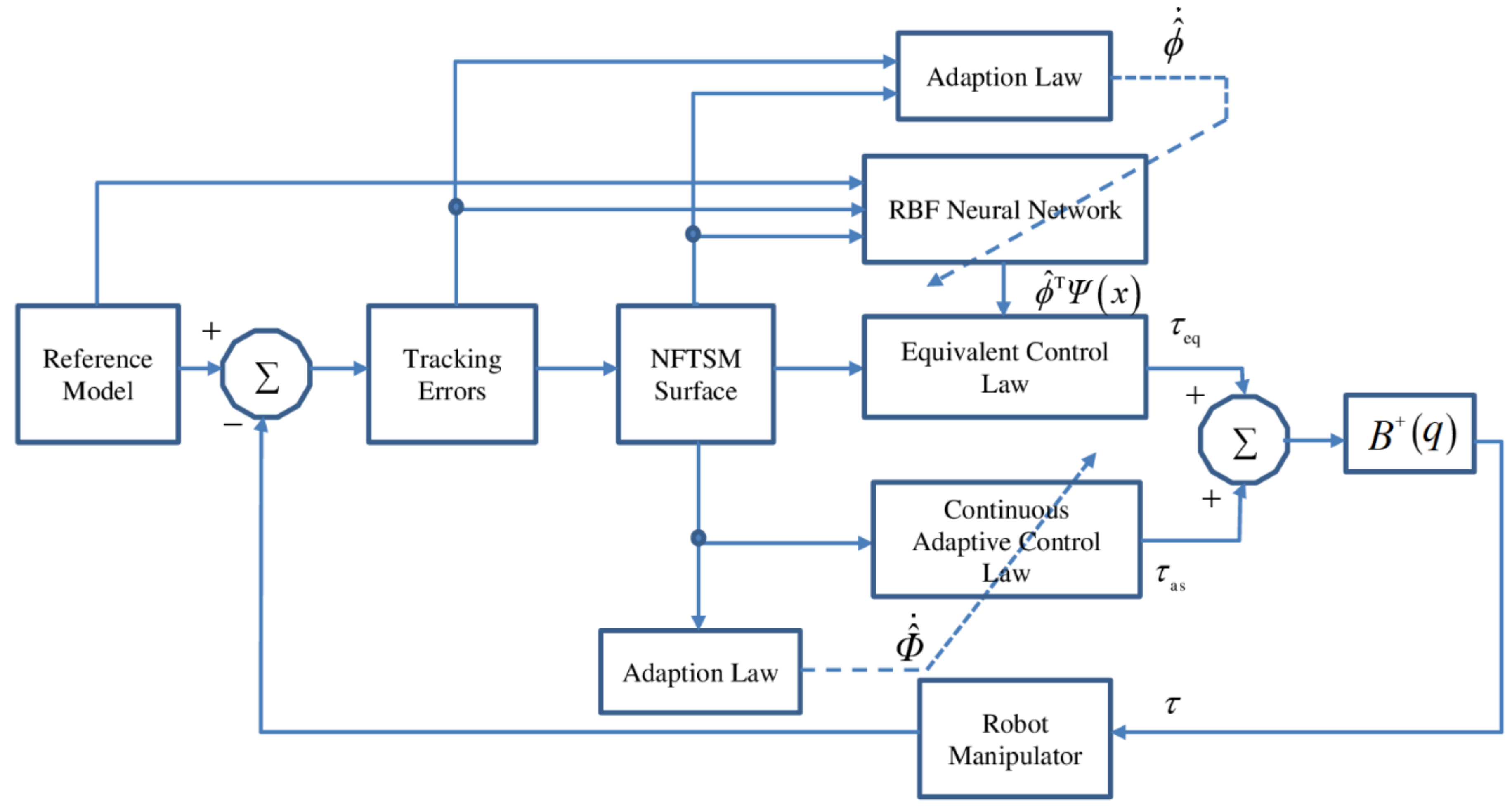
The proposed control law as depicted in Figure 2 is designed as follows:
τ ( t ) = B + ( q ) ( τ e q ( t ) + τ a s ( t ) ) .
Here, the equivalent control law is constructed as
τ e q ( t ) = ( ϕ ^ T Ψ ( x ) + Π ( e , ς ) q ¨ d ) ,
and τ a s ( t ) is an adaptive control term for replacing the control law τ s ( t ) in Equation (32), describing τ a s ( t ) as
τ a s = ( Φ ^ + ρ 1 ) s i g n ( s ) ,
and the adaptive updating rules are given as
Φ ^ ˙ = 1 γ | s | ,
ϕ ^ ˙ = 1 ω s Ψ ( x ) ,
where Φ ^ is the estimated value of the design parameter Φ , ρ 1 is a positive constant, and γ , ω indicate the adaptive gains.
The control design approach for the robot system is summarized in Theorem 3 below.
Theorem 3.
For the system (3), if the suitable NFTSM variables have been selected as (7) and (8) and the control input signal is constructed as (41)–(43) with its parameter updating rules designed as (44) and (45), then the sliding variable motion is a certainty, and the tracking error variables converge to zero.
Proof. 
Define the adaptive estimation error and NN weight approximation error, respectively, as follows
Φ ˜ = Φ ^ Φ ,
ϕ ˜ = ϕ ϕ ^ .
 □
The time derivative of the sliding surface in Equation (29) is rewritten as
s ˙ = ϕ Ψ ( x ) + B ( q ) τ ( t ) + W q ¨ d + Π ( e , ς ) .
Substituting control laws (41)–(43) into Equation (48) provides
s ˙ = ϕ ˜ T Ψ ( x ) ( Φ ^ + ρ 1 ) s i g n ( s ) + W .
The positive-definite Lyapunov functional is selected as
V 4 = s T s 2 + γ Φ ˜ T Φ ˜ 2 + ω ϕ ˜ T ϕ ˜ 2 .
With the result of Equation (49), the time derivative of Equation (50) is derived as
V ˙ 4 = s T s ˙ + γ Φ ˜ T Φ ˜ ˙ ω ϕ ˜ T ϕ ^ ˙ = s T ( ϕ ˜ T Ψ ( x ) ( Φ ^ + ρ 1 ) s i g n ( s ) + W ) + γ ( Φ ^ Φ ) Φ ^ ˙ ω ϕ ˜ T ϕ ^ ˙ = s T ϕ ˜ T Ψ ( x ) Φ ^ | s | ρ 1 | s | + W s + γ ( Φ ^ Φ ) Φ ^ ˙ ω ϕ ˜ T ϕ ^ ˙ .
Applying the updating laws (41)–(43) to (51) yields
V ˙ 4 = Φ ^ | s | ρ 1 | s | + Φ s + ( Φ ^ Φ ) | s | = ρ 1 | s | + W s Φ | s | ρ 1 | s | .
If the parameter ρ 1 is selected to be greater than zero, V ˙ 4 will be negative-definite. Based on the Lyapunov principle [47], V ˙ 4 becoming negative-definite indicates that s and Φ ˜ reach zero. Therefore, the tracking error variables converge to the sliding variables. Therefore, Theorem 3 is proven.
Remark 2.
In practical systems, the parameter drift problem typically occurs under the adaptive control rule (44). Consequently, the bounded approach is implemented to set up the adaptive estimator as
Φ ^ ˙ = { 0 if | s | ϖ 1 γ | s | if | s | > ϖ ,
in which ϖ > 0 is an arbitrary positive value.
Remark 3.
[35]: The chattering phenomenon can be significantly alleviated by replacing the s i g n ( ) function with a saturation function in the control input signal, such as
sat ( s ε ) = { s i g n ( s ) if   | s | ( ε ) 2 s ε if   | s | < ε
in which 0 < ε < 1 is a minor positive coefficient called boundary layer thickness, and ε = 0.1 .

4. Simulation Analyses

To demonstrate the effectiveness of the proposed control strategy, the strategy was applied to a pathway tracking control for the first three joints of a PUMA560 manipulator, and its tracking performance was compared with those of a classical SMC [16,17] and NFTSMC [49,50]. The dynamic model with the crucial parameters found in a 3-DOF PUMA560 robot manipulator was explained by Armstrong et al. [51]. We utilized the MATLAB/Simulink environment for all simulation analysis with the sampling rate set to 10 3 s. In this work, only the first three joints of a robot manipulator were investigated (the last three joints were blocked). The simulations were implemented to compare the controllers in terms of their positional accuracy, response speed, and the resulting chattering phenomenon in their control inputs.
To ascertain the robustness of all control methods, we evaluated the system performance in three operation stages, where disturbances and uncertainties were modeled as follows:
F r ( q ˙ ) + τ d ( t ) = [ 0.9 q ˙ 1 + 1.0 sin ( 3 q 1 ) + 1.7 sin ( q ˙ 1 ) 1.8 q ˙ 2 + 1.85 sin ( 2 q 2 ) + 1.65 sin ( q ˙ 2 ) 2.1 q ˙ 3 + 2.5 sin ( 2 q 3 ) + 0.57 sin ( q ˙ 3 ) ] .
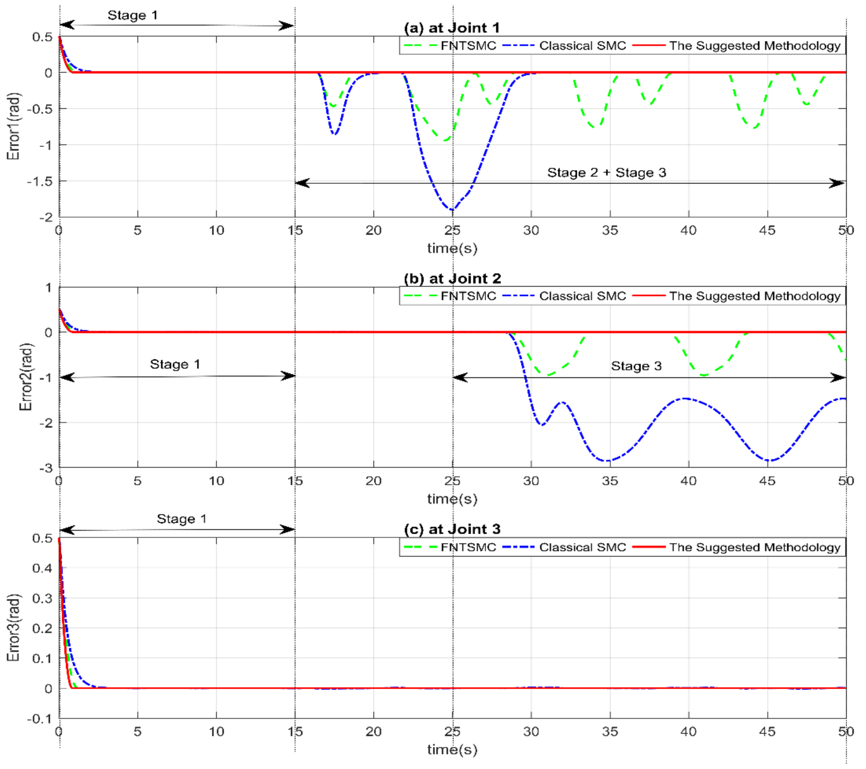
Stage 1: Robot system was assumed to run under normal operation from time 0 s to 15 s.
Stage 2: Robot system was assumed to run under operation condition, but there was an external disturbance impacting the first joint between 15 s and 50 s. This external disturbance had a value defined as ( 15 sin ( q 1 q 2 ) + 1.5 cos ( q ˙ 1 q 2 ) + 5.5 cos ( q ˙ 1 q ˙ 2 ) ) .
Stage 3: Robot system was assumed to run under operation condition, but there was a partial loss (75%) of control input effectiveness at the second joint between 25 s and 50 s.
The desired joint pathways for the position tracking were
q r = [ cos ( t 5 π ) 1 , sin ( t 5 π + π 2 ) , sin ( t 5 π + π 2 ) 1 ] T .
The RBFNN architecture consisted of seven nodes, the initial weight matrix of the network was selected as 0, the width and center of the Gaussian function was set as δ = 0.2 , and the center of the Gaussian function μ was selected in range (−1.5 ÷ 1.5) with μ l = 0.5 . The matrix used in an adaptive law of RBFNN was selected as ω = 15 I 7 , and the NN input was selected as υ = [ e e ˙ q r q ˙ r q ¨ r ] .
The SMC control input was set as
τ ( t ) = B 1 ( q ) ( Ξ ( q , q ˙ ) + η ( q ˙ q ˙ r ) q ¨ r + ( Φ 2 + ρ 2 ) s i g n ( s ) ) .
Here, η , Φ 2 , ρ 2 are positive constants, s is a linear sliding function, and q r is defined as a desired trajectory value.
The NFTSMC control input was set as
τ ( t ) = B 1 ( q ) ( Ξ ( q , q ˙ ) q ¨ r + β h d ( e ˙ ) 2 d h + ( Φ 3 + ρ 3 ) s s + ν ) .
Here, β , Φ 3 , ρ 3 are positive constants, s is a nonlinear sliding function, ν is a small positive scalar, q r is defined as a desired trajectory value, and d ,   h are positive odd integers satisfying the condition 1 < d / h < 2 .
The control parameter selection for the varying control strategies, including classical SMC, NTSMC, and the proposed control strategy is shown in Table 1.
The averaged tracking errors were calculated according to the following equation E i a v = 1 n k = 1 n ( e i 2 )   i = 1 ,   2 ,   3 in which n is the number of simulation steps.
The trajectory tracking performances, including tracking positions and tracking errors at each of the first three joints with three controllers, are illustrated in Figure 3 and Figure 4. In Stage 1 (from 0 s to 15 s), three of the control systems give similar good path tracking performance. In Stage 2 (from time greater than 15 s) and in Stage 3 (from time greater than 25 s), it is clear that the classical SMC provides the poorest path tracking performance, where robot operation becomes unstable when a large disturbance or uncertainty is applied. From Table 2 and Figure 4, it is observed that NFTSMC provides less path tracking error and faster transient response than classical SMC. However, tracking performance is also diminished upon application of a large disturbance. It is noteworthy that the proposed sliding surface is designed based on the sliding function integral in Equation (8), and this integral portion has a significant role in providing fast transient response and robustness against uncertainty and disturbances. Therefore. the proposed control strategy gives the best path tracking performance and fastest transient response among the compared control strategies, due to the role of the proposed surfaces, an adaptive compensator, and a main contribution of the proposed controller.
The control input signals for all control types, including classical SMC, NFTSMC, and the suggested system are shown in Figure 5. In Figure 5a, it is clear that the NFTSMC offers a continuous control signal by using a boundary technique [35]. However, the weakness of this technique is that a choice must be made between chattering phenomenon removal and path tracking precision. Consequently, this technique decreases the robustness of the system while also increasing the tracking error. In Figure 5b, the SMC offers a discontinuous control signal with serious chattering behavior. On the contrary, the suggested system offers a continuous control signal for the robot manipulator without the loss of its effectiveness, as shown in Figure 5c.
The adaptations of the estimated parameters are shown in Figure 6. These adaptive gains are estimated according to the variation of the influences of disturbances and uncertainties, and they will attain a constant value once the error variables converge to the sliding surface in a stable phase.
From the simulation performance, we conclude that the proposed controller gives the best performance compared to a classical SMC and NFTSMC in terms of tracking precision, transient response, chattering deletion, and small steady state error.

5. Conclusions

In this report, a robust trajectory tracking control strategy was developed for robot manipulators. From the simulation results and performance comparison with two other control strategies for a 3-DOF PUMA560 robot manipulator, our control strategy offered the best performance in terms of tracking positional accuracy, small steady-state errors, fast convergence, and chattering phenomenon rejection. The suggested control solution has the following benefits: (1) inherits the advantages of the NFTSMC, including non-singularity, finite-time convergence, fast transient response, low steady-state errors, and high position tracking accuracy; (2) achieves smoothness with elimination of chattering behavior; (3) does not demand an exact dynamic model for the robot manipulator by applying an adaptive radial basis function neural network to approximate an unknown robot function; (4) compared to the classical SMC and another control methods based on TSMC, the proposed control strategy offers better tracking performance and stronger resistance against disturbances and uncertainties; (5) robustness and stability of the robot system was demonstrated fully by Lyapunov theory.

Author Contributions

All authors contributed equally to this article and accepted the final report.

Funding

This research was funded by the Ministry of Education, grant number (NRF-2016R1D1A3B03930496).

Acknowledgments

This work was supported by the Basic Science Research Program through the National Research Foundation of Korea (NRF) funded by the Ministry of Education (NRF-2016R1D1A3B03930496).

Conflicts of Interest

All authors announce that they have no conflict of interest in relation to the publication of this article.

References

  1. Yang, C.; Huang, Q.; Jiang, H.; Peter, O.O.; Han, J. PD control with gravity compensation for hydraulic 6-DOF parallel manipulator. Mech. Mach. Theory 2010, 45, 666–677. [Google Scholar] [CrossRef]
  2. Ouyang, P.R.; Zhang, W.-J.; Wu, F.-X. Nonlinear PD control for trajectory tracking with consideration of the design for control methodology. In Proceedings of the IEEE International Conference on Robotics and Automation, ICRA’02, Washington, DC, USA, 10–17 May 2002; Volume 4, pp. 4126–4131. [Google Scholar]
  3. Arimoto, S. Stability and robustness of PID feedback control for robot manipulators of sensory capability. In Proceedings of the Robotics Research: The First International Symposium, Bretton Woods, NH, USA, 25 August–2 September 1983; pp. 783–799. [Google Scholar]
  4. Su, Y.; Müller, P.C.; Zheng, C. Global Asymptotic Saturated PID Control for Robot Manipulators. IEEE Trans. Control Syst. Technol. 2010, 18, 1280–1288. [Google Scholar] [CrossRef]
  5. Guo, Y.; Woo, P.-Y. An adaptive fuzzy sliding mode controller for robotic manipulators. IEEE Tran. Syst. Man Cybern.-Part A Syst. Hum. 2003, 33, 149–159. [Google Scholar]
  6. Tran, X.-T.; Kang, H.-J. TS fuzzy model-based robust finite time control for uncertain nonlinear systems. Proc. Inst. Mech. Eng. Part C J. Mech. Eng. Sci. 2015, 229, 2174–2186. [Google Scholar] [CrossRef]
  7. Vo, A.T.; Kang, H.-J.; Le, T.D. An Adaptive Fuzzy Terminal Sliding Mode Control Methodology for Uncertain Nonlinear Second-Order Systems. In Proceedings of the International Conference on Intelligent Computing, Wuhan, China, 15–18 August 2018; pp. 123–135. [Google Scholar]
  8. Sanger, T.D. Neural network learning control of robot manipulators using gradually increasing task difficulty. IEEE Trans. Robot. Autom. 1994, 10, 323–333. [Google Scholar] [CrossRef]
  9. Hsia, T.C.; Jung, S. A simple alternative to neural network control scheme for robot manipulators. IEEE Trans. Ind. Electron. 1995, 42, 414–416. [Google Scholar] [CrossRef]
  10. Vo, A.T.; Kang, H.-J.; Nguyen, V.-C. An output feedback tracking control based on neural sliding mode and high order sliding mode observer. In Proceedings of the 2017 10th International Conference on Human System Interactions (HSI), Ulsan, Korea, 17–19 July 2017; pp. 161–165. [Google Scholar]
  11. Van, M.; Kang, H.-J.; Suh, Y.-S.; Shin, K.-S. A robust fault diagnosis and accommodation scheme for robot manipulators. Int. J. Control Autom. Syst. 2013, 11, 377–388. [Google Scholar] [CrossRef]
  12. Shang, W.; Cong, S. Nonlinear computed torque control for a high-speed planar parallel manipulator. Mechatronics 2009, 19, 987–992. [Google Scholar] [CrossRef]
  13. Zhihong, M.; O’day, M.; Yu, X. A robust adaptive terminal sliding mode control for rigid robotic manipulators. J. Intell. Robot. Syst. 1999, 24, 23–41. [Google Scholar] [CrossRef]
  14. Moreno, J.A.; Negrete, D.Y.; Torres-González, V.; Fridman, L. Adaptive continuous twisting algorithm. Int. J. Control 2016. [Google Scholar] [CrossRef]
  15. Lim, K.; Eslami, M. Robust adaptive controller designs for robot manipulator systems. IEEE J. Robot. Autom. 1987, 3, 54–66. [Google Scholar] [CrossRef]
  16. Utkin, V.I. Sliding Modes in Control and Optimization; Springer Science & Business Media: Berlin, Germany, 2013. [Google Scholar]
  17. Edwards, C.; Spurgeon, S. Sliding Mode Control: Theory and Applications; Crc Press: Boca Raton, FL, USA, 1998. [Google Scholar]
  18. Eker, I. Sliding mode control with PID sliding surface and experimental application to an electromechanical plant. ISA Trans. 2006, 45, 109–118. [Google Scholar] [CrossRef]
  19. Kamal, S.; Moreno, J.A.; Chalanga, A.; Bandyopadhyay, B.; Fridman, L.M. Continuous terminal sliding-mode controller. Automatica 2016. [Google Scholar] [CrossRef]
  20. Xiao, B.; Hu, Q.; Zhang, Y. Adaptive sliding mode fault tolerant attitude tracking control for flexible spacecraft under actuator saturation. IEEE Trans. Control Syst. Technol. 2012, 20, 1605–1612. [Google Scholar] [CrossRef]
  21. Man, Z.; Paplinski, A.P.; Wu, H.R. A robust MIMO terminal sliding mode control scheme for rigid robotic manipulators. IEEE Trans. Autom. Control 1994, 39, 2464–2469. [Google Scholar] [CrossRef]
  22. Wu, Y.; Yu, X.; Man, Z. Terminal sliding mode control design for uncertain dynamic systems. Syst. Control Lett. 1998, 34, 281–287. [Google Scholar] [CrossRef]
  23. Tang, Y. Terminal sliding mode control for rigid robots. Automatica 1998, 34, 51–56. [Google Scholar] [CrossRef]
  24. Yu, X.; Zhihong, M. Fast terminal sliding-mode control design for nonlinear dynamical systems. Circuits Syst. I Fundam. Theory 2002, 49, 261–264. [Google Scholar] [CrossRef]
  25. Mobayen, S. Fast terminal sliding mode controller design for nonlinear second-order systems with time-varying uncertainties. Complexity 2015, 21, 239–244. [Google Scholar] [CrossRef]
  26. Madani, T.; Daachi, B.; Djouani, K. Modular-controller-design-based fast terminal sliding mode for articulated exoskeleton systems. IEEE Trans. Control Syst. Technol. 2017, 25, 1133–1140. [Google Scholar] [CrossRef]
  27. Eshghi, S.; Varatharajoo, R. Nonsingular terminal sliding mode control technique for attitude tracking problem of a small satellite with combined energy and attitude control system (CEACS). Aerosp. Sci. Technol. 2018, 76, 14–26. [Google Scholar] [CrossRef]
  28. Safa, A.; Abdolmalaki, R.Y.; Shafiee, S.; Sadeghi, B. Adaptive nonsingular terminal sliding mode controller for micro/nanopositioning systems driven by linear piezoelectric ceramic motors. ISA Trans. 2018. [Google Scholar] [CrossRef] [PubMed]
  29. Lin, C.-K. Nonsingular terminal sliding mode control of robot manipulators using fuzzy wavelet networks. IEEE Trans. Fuzzy Syst. 2006, 14, 849–859. [Google Scholar] [CrossRef]
  30. Su, Y.; Zheng, C.; Mercorelli, P. Global finite-time stabilization of planar linear systems with actuator saturation. IEEE Trans. Circuits Syst. II Express Briefs 2017, 64, 947–951. [Google Scholar] [CrossRef]
  31. Su, Y.; Zheng, C. Robust finite-time output feedback control of perturbed double integrator. Automatica 2015, 60, 86–91. [Google Scholar] [CrossRef]
  32. Xu, S.S.-D.; Chen, C.-C.; Wu, Z.-L. Study of nonsingular fast terminal sliding-mode fault-tolerant control. IEEE Trans. Ind. Electron. 2015, 62, 3906–3913. [Google Scholar] [CrossRef]
  33. Yang, L.; Yang, J. Nonsingular fast terminal sliding-mode control for nonlinear dynamical systems. Int. J. Robust Nonlinear Control 2011, 21, 1865–1879. [Google Scholar] [CrossRef]
  34. Chen, G.; Jin, B.; Chen, Y. Nonsingular fast terminal sliding mode posture control for six-legged walking robots with redundant actuation. Mechatronics 2018, 50, 1–15. [Google Scholar] [CrossRef]
  35. Utkin, V. Discussion aspects of high-order sliding mode control. IEEE Trans. Autom. Control 2016, 61, 829–833. [Google Scholar] [CrossRef]
  36. Feng, Y.; Zhou, M.; Zheng, X.; Han, F.; Yu, X. Full-order terminal sliding-mode control of MIMO systems with unmatched uncertainties. J. Frankl. Inst. 2018, 355, 653–674. [Google Scholar] [CrossRef]
  37. Feng, Y.; Han, F.; Yu, X. Chattering free full-order sliding-mode control. Automatica 2014, 50, 1310–1314. [Google Scholar] [CrossRef]
  38. Rubio-Astorga, G.; Sánchez-Torres, J.D.; Cañedo, J.; Loukianov, A.G. High-order sliding mode block control of single-phase induction motor. IEEE Trans. Control Syst. Technol. 2014, 22, 1828–1836. [Google Scholar] [CrossRef]
  39. Nentwig, M.; Mercorelli, P. Throttle valve control using an inverse local linear model tree based on a fuzzy neural network. In Proceedings of the 7th IEEE International Conference on Cybernetic Intelligent Systems, London, UK, 9–10 September 2008; pp. 1–6. [Google Scholar]
  40. Li, X.-J.; Yang, G.-H. Neural-network-based adaptive decentralized fault-tolerant control for a class of interconnected nonlinear systems. IEEE Trans. Neural Netw. Learn. Syst. 2018, 29, 144–155. [Google Scholar] [CrossRef] [PubMed]
  41. Sun, R.; Wang, J.; Zhang, D.; Shao, X. Neural network-based sliding mode control for atmospheric-actuated spacecraft formation using switching strategy. Adv. Space Res. 2018, 61, 914–926. [Google Scholar] [CrossRef]
  42. Shen, Q.; Jiang, B.; Cocquempot, V. Adaptive fuzzy observer-based active fault-tolerant dynamic surface control for a class of nonlinear systems with actuator faults. IEEE Trans. Fuzzy Syst. 2014, 22, 338–349. [Google Scholar] [CrossRef]
  43. Huo, B.; Xia, Y.; Yin, L.; Fu, M. Fuzzy adaptive fault-tolerant output feedback attitude-tracking control of rigid spacecraft. IEEE Trans. Syst. Man Cybern. Syst. 2017, 47, 1898–1908. [Google Scholar] [CrossRef]
  44. Wang, S.-Y.; Liu, F.-Y.; Chou, J.-H. Adaptive TSK fuzzy sliding mode control design for switched reluctance motor DTC drive systems with torque sensorless strategy. Appl. Soft Comput. 2018, 66, 278–291. [Google Scholar] [CrossRef]
  45. Spong, M.W.; Vidyasagar, M. Robot Dynamics and Control; John Willey & Sons: New York, NY, USA, 1989. [Google Scholar]
  46. Islam, S.; Liu, X.P. Robust sliding mode control for robot manipulators. IEEE Trans. Ind. Electron. 2011, 58, 2444–2453. [Google Scholar] [CrossRef]
  47. Polyakov, A.; Fridman, L. Stability notions and Lyapunov functions for sliding mode control systems. J. Frankl. Inst. 2014, 351, 1831–1865. [Google Scholar] [CrossRef]
  48. Bhat, S.P.; Bernstein, D.S. Finite-time stability of continuous autonomous systems. SIAM J. Control Opt. 2000, 38, 751–766. [Google Scholar] [CrossRef]
  49. Yu, S.; Yu, X.; Shirinzadeh, B.; Man, Z. Continuous finite-time control for robotic manipulators with terminal sliding mode. Automatica 2005, 41, 1957–1964. [Google Scholar] [CrossRef]
  50. Feng, Y.; Yu, X.; Man, Z. Non-singular terminal sliding mode control of rigid manipulators. Automatica 2002, 38, 2159–2167. [Google Scholar] [CrossRef]
  51. Armstrong, B.; Khatib, O.; Burdick, J. The explicit dynamic model and inertial parameters of the PUMA 560 arm. In Proceedings of the 1986 IEEE International Conference on Robotics and Automation, San Francisco, CA, USA, 7–10 April 1986; Volume 3, pp. 510–518. [Google Scholar]
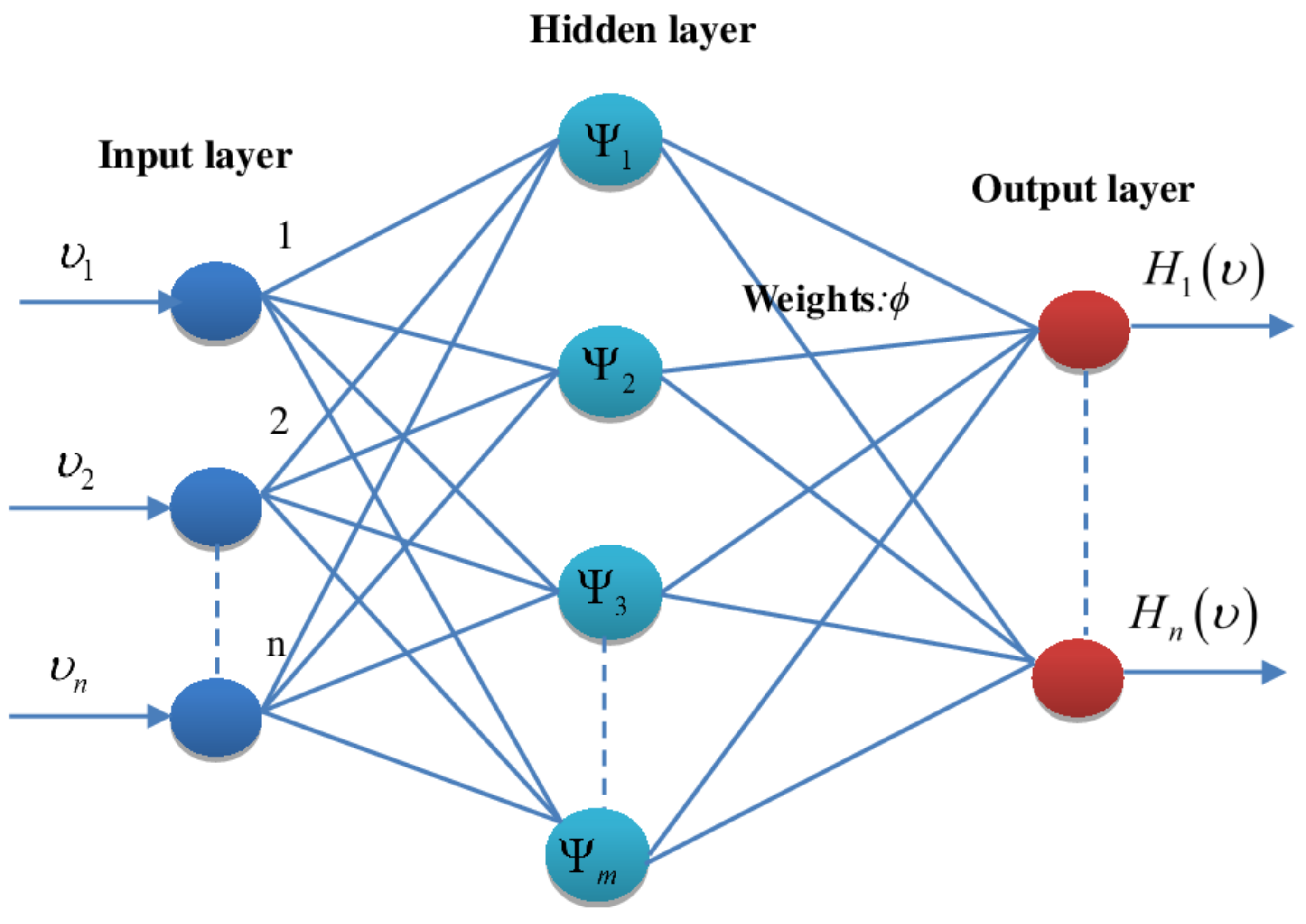
Figure 1. Structure of radial basis function neural network.
Applsci 08 02562 g001
Figure 2. Block diagram of the proposed control method. RBR = radial basis function; NFTSM = nonsingular fast terminal sliding mode control.
Applsci 08 02562 g002
Figure 3. Trajectory tracking positions: (a) at Joint 1, (b) at Joint 2, and (c) at Joint 3.
Applsci 08 02562 g003
Figure 4. Trajectory tracking errors: (a) at Joint 1, (b) at Joint 2, and (c) at Joint 3.
Applsci 08 02562 g004
Figure 5. Control input signals: (a) FNTSMC, (b) classical SMC, and (c) the suggested control methodology. FNTSMC = fast nonsingular terminal sliding mode control.
Applsci 08 02562 g005
Figure 6. Time history of adaptive gain.
Applsci 08 02562 g006
Table 1. The control parameter selection for the varying control strategies. SMC = sliding mode controller; ANNFTSMC = adaptive neural non-singular fast-terminal sliding-mode control.
Control StrategyControl ParametersParameter Value
Classical SMC η , Φ 2 , ρ 2 2, 9.9, 1
NFTSMC d , h , β 5, 3, 2
Φ 3 , ρ 3 , ν 9.9, 1, 0.1
Proposed Control Strategy (ANNFTSMC) h 1 , h 2 d i a g ( 10 , 10 , 10 ) , d i a g ( 6 , 6 , 6 )
Γ 1 , Γ 2 , Γ 3 d i a g ( 3 , 3 , 3 ) , d i a g ( 3 , 3 , 3 ) , d i a g ( 2 , 2 , 2 )
ϑ , α d i a g ( 0.4 , 0.4 , 0.4 ) , d i a g ( 1.2 , 1.2 , 1.2 )
γ , ρ 1 , ϖ , ε 0.5, 0.1, 0.01, 0.1
Table 2. The averaged tracking errors under control input signals of the control strategy.
Error Control Strategy E 1 a v E 2 a v E 3 a v
SMC 0.1943 0.8708 0.0060
NFTSMC 0.1542 0.1218 0.0038
ANNFTSMC 0.0031 0.0031 0.0029