A Graph Representation Composed of Geometrical Components for Household Furniture Detection by Autonomous Mobile Robots

Abstract

This study proposes a framework to detect and recognize household furniture using autonomous mobile robots. The proposed methodology is based on the analysis and integration of geometric features extracted over 3D point clouds. A relational graph is constructed using those features to model and recognize each piece of furniture. A set of sub-graphs corresponding to different partial views allows matching the robot’s perception with partial furniture models. A reduced set of geometric features is employed: horizontal and vertical planes and the legs of the furniture. These features are characterized through their properties, such as: height, planarity and area. A fast and linear method for the detection of some geometric features is proposed, which is based on histograms of 3D points acquired from an RGB-D camera onboard the robot. Similarity measures for geometric features and graphs are proposed, as well. Our proposal has been validated in home-like environments with two different mobile robotic platforms; and partially on some 3D samples of a database.

1. Introduction

Nowadays, the use of service robots is more frequent in different environments for performing tasks such as: vacuuming floors, cleaning pools or mowing the lawn. In order to provide more complex and useful services, robots need to identify different objects in the environment; but also, they must understand the uses, relationships and characteristics of objects in the environment.

The extraction of an object’s characteristics and its spatial relationships can help a robot to understand what makes an object useful. For example, the largest surfaces of a table and a bed differ in planarity and height; then, modeling object’s characteristics can help the robot to identify their differences. A robot with a better understanding of the world is a more efficient service robot.

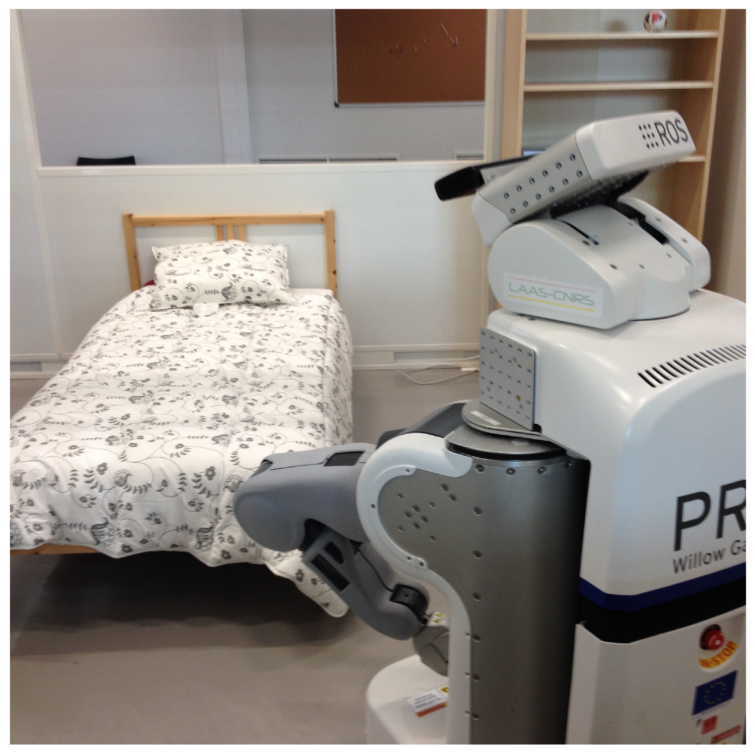
A robot can reconstruct the environment geometry through the extraction of geometrical structures on indoor scenes. Wall, floor or ceiling extractions are already widely used for environment characterization; however, there are few studies on extracting the geometric characteristics of furniture. Generally, the extraction is performed on very large scenes, composed of multiple scans and points of view, while we extract the geometric characteristics of furniture from only a single point of view (Figure 1).

Human environments are composed of many type of objects. Our study focuses on household furniture that can be moved by a typical human and that is designed to be moved during normal usage.

Our study omits kitchen furniture, fixed bookcases, closets or other static or fixed objects; because they can be categorized in the map as fixed components, therefore, the robot will always know their position. The frequency each piece of furniture is repositioned will vary widely: a chair is likely to move more often than a bed. Furthermore, the magnitude of repositioning a piece of furniture will vary widely: the intentional repositioning of a chair will likely move farther than the incidental repositioning of a table.

When an object is repositioned, if the robot does not extract the new position of the object and update its knowledge of the environment, then the robot’s localization will be less accurate.

The main idea is to model these pieces of furniture (offline) in order to detect them on execution time and add them to the map simultaneously, not as obstacles, but as objects with semantic information that the robot could use later.

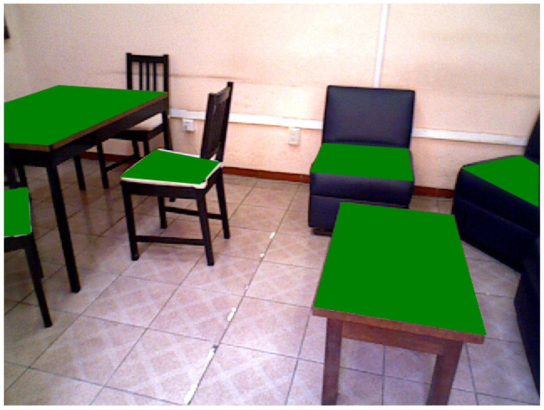
In this work, the object’s horizontal or quasi-horizontal planes are key features (Figure 2). These planes are common in home environments: for sitting at a table, for lounging, or to support another object. The main difference between various planes is whether the horizontal plane is a regular or irregular flat surface. For example, the horizontal plane of a dining table or the horizontal plane of the top of a chest of drawers is different from the horizontal plane of a couch or the horizontal plane of a bed.

Modeling these planes can help a robot to detect those objects and to understand the world. It can help a robot, for example, to know where it can put a glass of water.

This work proposes that each piece of furniture is modeled with graphs. The nodes represent geometrical components, and the arcs represent the relationships between the nodes. Each graph of a piece of furniture has a main node representing a horizontal plane, generally the horizontal plane most commonly used by a human. Furthermore, this principle vertex is normally the horizontal plane a typical human can view from a regular perspective (Figure 2). In our framework, we take advantage of the fact that the horizontal plane most easily viewed by a typical human is usually the horizontal plane most used by a human. The robot has cameras positioned to provide the robot with a point of view similar to the point of view of a typical human.

To recognize the furniture, the robot uses an RGB-D camera to acquire three-dimensional data from the environment. After acquiring 3D data, the robot extracts the geometrical components and creates a graph for each object in the scene. Because the robot maintains the relationships between all coordinates of its parts, the robot can transform the point cloud to a particular reference frame, which simplifies the extraction of geometric components; specifically, to the robot’s footprint reference frame.

From transformed point clouds of a given point of view, the robot extracts graphs corresponding to partial views for each piece of furniture in the scene. The graphs generated are later compared with the graphs of the object’s models contained in a database.

The main contributions of this study are:

• a graph representation adapted to detect pieces of furniture using an autonomous mobile robot;
• a representation of partial views of furniture models given by sub-graphs;
• a fast and linear method for geometric feature extraction (planes and poles);
• metrics to compare the partial views and characteristics of geometric components; and
• a process to update the environment map when furniture is repositioned.

2. Related Work

RGB-D sensors have been widely used in robots; therefore, they are excellent for extracting information about diverse tasks in diverse environments. These sensors have been employed to solve many tasks; e.g., to construct 3D environments, for object detection and recognition and in human-robot interaction. For many tasks, but particularly when mobile robots must detect objects or humans, the task must be solved in real time or near real time; therefore, the rate at which the robot processes information is a key factor. Hence, an efficient 3D representation of objects that can quickly and accurately detect them is important.

Depending on the context or the environment, there are different techniques to detect and represent 3D objects. The most common techniques are based on point features.

The extraction of some 3D features is already available in libraries like Point Cloud Library (PCL) [1], including: spin images or fast point feature histograms. Those characteristics provide good results as the quantity of points increases. An increase in points, however, increases the computational time. A large object, such as furniture, requires computational times that are problematic for real-time tasks. A comparative evaluation of PCL 3D features on point clouds was given in [2].

The use of RGB-D cameras for detecting common objects (e.g., hats, cups, cans, etc.) has been accomplished by many research teams around the world. For example, a study [3] presented an approach based on depth kernel features that capture characteristics such as size, shape and edges. Another study [4] detected objects by combining sliding window detectors and 3D shape.

Others works ([5,6]) have followed a similar approach using features to detect other types of free-form objects. For instance, in [5], 3D-models were created and objects detected simultaneously by using a local surface feature. Additionally, local features in a multidimensional histogram have been combined to classify objects in range images [6]. These studies used specific features extracted from the objects and then compared the extracted features with a previously-created database, containing the models of the objects.

Furthermore, other studies have performed 3D object-detection based on pairs of points from oriented surfaces. For example, Wahl et al. [7] proposed a four-dimensional feature invariant to translation and rotation, which captures the intrinsic geometrical relationships; whereas Drost et al. [8] have proposed a global-model description based on oriented pairs of points. These models are independent from local surface-information, which improves search speed. Both methods are used to recognize 3D free-form objects in CAD models.

In [9], the method presented in [8] was applied to detect furniture for an “object-oriented” SLAM technique. By detecting multiple repetitive pieces of furniture, the classic SLAM technique was extended. However, they used a limited range of types of furniture, and a poor detection of furniture was reported when the furniture was distant or partially occluded.

On the other hand, Wu et al. [10] proposed a different object representation to recognize and reconstruct CAD models from pieces of furniture. Specifically, they proposed to represent the 3D shape of objects as a probability distribution of binary variables on a 3D voxel grid using a convolutional deep belief network.

As stated in [11], it is reasonable to represent an indoor environment as a collection of planes because a typical indoor environment is mostly planar surfaces. In [12], using a 3D point cloud and 2D laser scans, planar surfaces were segmented, but those planes are used only as landmarks for map creation. In [13], geometrical structures are used to describe the environment. In this work, using rectangular planes and boxes, a kitchen environment is reconstructed in order to provide to the robot a map with more information about, i.e., how to use or open a particular piece of furniture.

A set of planar structures to represent pieces of furniture was presented in [14], which stated that their planar representations “have a certain size, orientation, height above ground and spatial relation to each other”. This method was used in [15] to create semantic maps of furniture. This method is similar to our framework; however, their method used a set of rules, while our method uses a probabilistic framework. Our method is more flexible, more able to deal with uncertainty, more able to process partial information and can be easily incorporated into many SLAM methods.

In relation to plane extraction, a faster alternative than the common methods for plane segmentation was presented in [16]. They used integral images, taking advantage of the structured point cloud from RGB-D cameras.

Another option is the use of semantic information from the environment to improve the furniture detection. For example in [17], geometrical properties of the 3D world and the contextual relations between the objects were used to detect objects and understand the environment. By using a Conditional Random Field (CRF) model, they integrated object appearance, geometry and relationships with the environment. This tackled some of the problems with feature-based approaches, including pose variation, object occlusion or illumination changes.

In [18], the use of the visual appearance, shape features and contextual relations such as object co-occurrence was proposed to semantically label a full 3D point cloud scene. To use this information, they proposed a graphical model isomorphic to a Markov random field.

The main idea of our approach is to improve the understanding of the environment by identifying the pieces of furniture, which is still a very challenging task, as stated in [19]. These pieces of furniture will be represented by a graph structure as a combination of geometrical entities.

Using graphs to represent environment relations was done in [20,21]. Particularly, in [20], a semantic model of the scene based on objects was created; where each node in the graph represented an object and the edges represented their relationship, which were also used to improve the object’s detection. The work in [21] used graphs to describe the configuration of basic shapes for the detection of features over a large point cloud. In this case, the nodes represent geometric primitives, such as planes, cylinders, spheres, etc.

Our approach uses a representation similar to [21]. Each object is decomposed into geometric primitives and represented by a graph. However, our approach differs because it processes only one point cloud at a time, and it is a probabilistic framework.

3. Furniture Model Representation and Similarity Measurements

Our proposal uses graphs to represent furniture models. Specifically, our approach focuses on geometrical components and relationships in the graph instead of a complete representation of the shape of the furniture.

Each graph contains the furniture’s geometrical components as nodes or a vertex. The edges or arcs represent the adjacency of the geometrical components. These geometrical components are described using a set of features that characterize them.

3.1. Furniture Graph Representation

A graph is defined as an ordered pair $G=(V,E)$ containing a set V of vertices or nodes and a set E of edges or arcs. A piece of furniture $F^i$ is represented by a graph as follows:

$$\begin{array}{cc}\hfill F^i=(V^i,E^i),& \mathrm{with}i=[1,\dots ,N_f]\hfill \end{array}$$

(1)

where $F^i$ is an element from the set of furniture models $\mathcal{F}$; the sets $V^i$ and $E^i$ contain the vertices and edges associated with the $i\mathrm{th}$ class; and $N_f$ is the number of models in the set $\mathcal{F}$, i.e., $\left|\mathcal{F}\right|=N_f$.

The set of vertices $V^i$ and the set of edges $E^i$ are described using lists as follows:

$$\begin{array}{cc}\hfill V^i& =\{v_1^i,v_2^i,\dots ,v_{n_v^i}^i\}\hfill \\ \hfill E^i& =\{e_1^i,e_2^i,\dots ,e_{n_e^i}^i\}\hfill \end{array}$$

(2)

where $n_v^i$ and $n_e^i$ are the number of vertices and edges, respectively, for the $i\mathrm{th}$ piece of furniture.

The functions $V(F^i)$ and $E(F^i)$ are used to recover the corresponding lists of vertex and edges of the graph $F^i$.

An edge $e_j^i$ is the $j\mathrm{th}$ link in the set, joining two nodes for the $i\mathrm{th}$ piece of furniture. As connections between nodes are a few, we use a simple list to store them. Thus, each edge $e_j^i$ is described as:

$$e_j^i=(a,b)$$

(3)

where a and b correspond to the linked vertices $v_a^i,v_b^i\in V^i$, such that $a\ne b$; and since the graph is an undirected graph, $e_j^i=(a,b)=(b,a)$.

3.2. Geometric Components

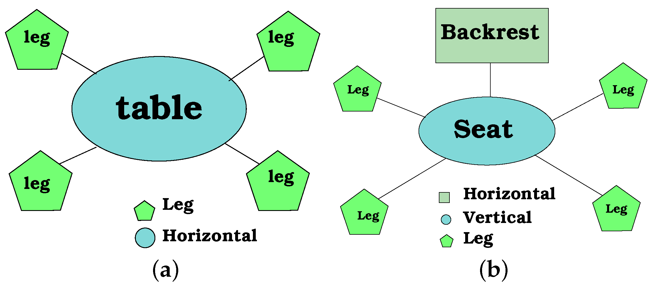
The vertices on a furniture graph model are geometric components, which roughly correspond to the different parts of the furniture. For instance, a chair has six geometric components: one horizontal plane for sitting, one vertical plane for the backrest and four tubes for the legs. Each component has different characteristics to describe it.

Generally, a geometric component $G{c}^k$ is a non-homogeneous set of characteristics:

$$G{c}^k=\{f{t}_1^k,f{t}_2^k,\dots ,f{t}_{n_{ft}^k}^k\}$$

(4)

where k designates an element from the set $\mathcal{G}c$, which contains $N_k$ different types of geometric components, and $n_{ft}^k$ is the number of characteristics of the $k\mathrm{th}$ geometric component. Characteristics or features of a geometrical component can be of various types or sources. A horizontal plane, for example, includes characteristics of height, area and relative measures.

Each vertex $v_j^i$ is then a geometric component of type k. The function $G_c(v_j^i)$ returns then the type and the set of features of geometric component k.

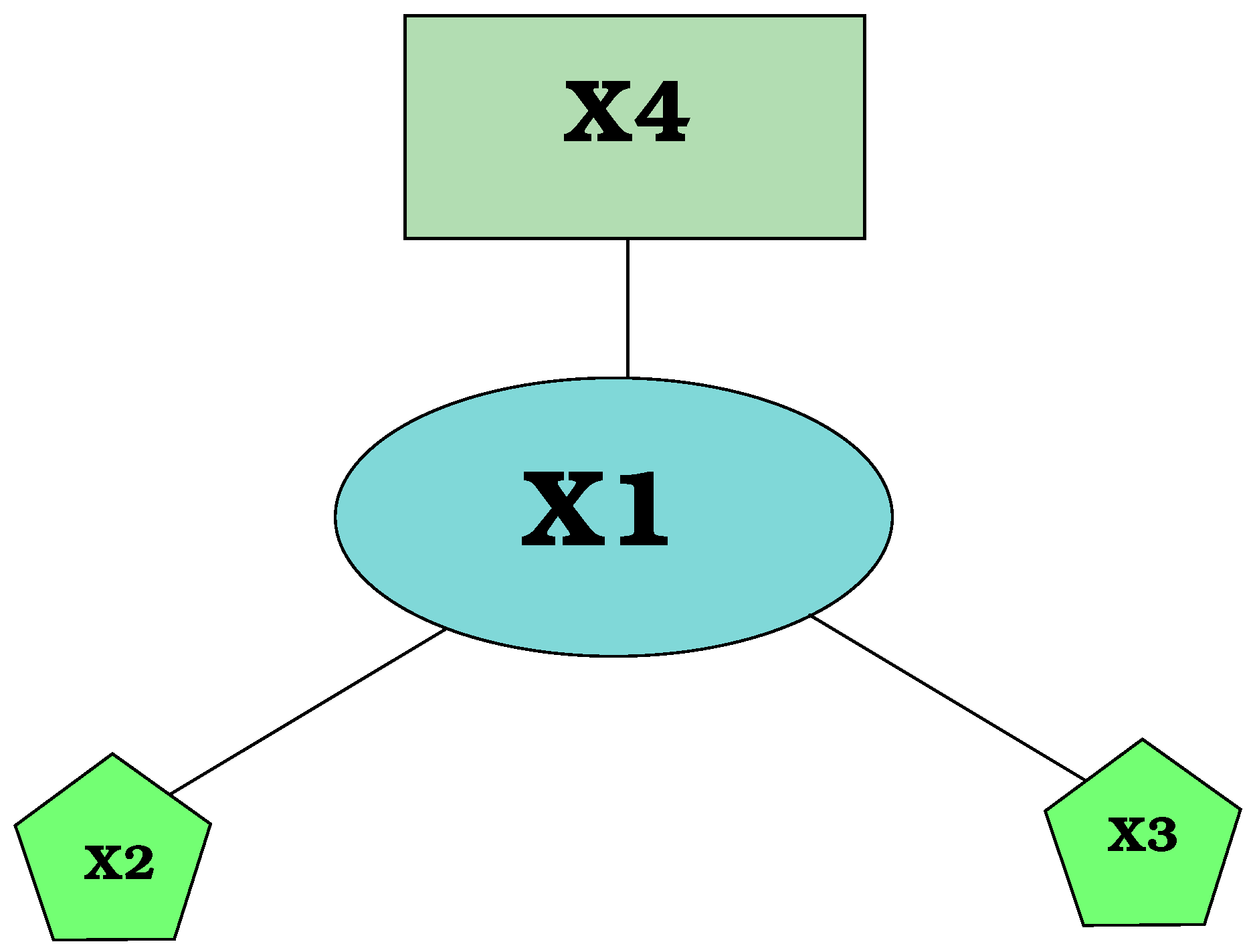
Figure 3 shows an example of a furniture model $F^i$. It is composed of four vertices ($n_v^i=4$) and three edges ($n_e^i=3$). There are three different types of vertices because each geometric component ($N_k=3$) is represented graphically with a different shape of the node.

Despite the simplified representation of the furniture, the robot cannot see all furniture components from a single position.

3.3. Partial Views

At any time, the robot’s perspective limits the geometric components the robot can observe. For each piece of furniture, the robot has a complete graph including every geometric component of the piece of furniture, then some subgraphs should be generated corresponding to different views that a robot can have. Each sub-graph contains the geometric components the robot would observe from a hypothetical perspective.

Considering the following definition, a graph H is called a subgraph of G, such that $V(H)\subseteq V(G)$ and $E(H)\subseteq E(G)$, then a partial view $F{p}^i$ for a piece of furniture is a subgraph from $F^i$, which is described as:

$$F{p}^i=({\tilde{V}}^i,{\tilde{E}}^i)$$

(5)

such that ${\tilde{V}}^i\subseteq V^i$ and ${\tilde{E}}^i\subseteq E^i$. The number of potential partial views is equal to the number of possible subsets in the set $F^i$; however, not all partial views are useful. See Section 4.3.

In order to match robot perception with the generated models, similarity measurements for graphs and geometric components should be defined.

3.4. Similarity Measurements

3.4.1. Similarity of Geometric Components

Generally, a similarity measure $s_{Gc}$ of two type k geometric components $G{c}^k$ and $G{c}^{k\prime }$ is defined as:

$$s_{Gc}^k(G{c}^k,G{c}^{k\prime })=1-\sum _i^{n_{ft}^k}{w}_{Gi}^{k}d(f{t}_i^k,f{t}_i^{k\prime })$$

(6)

where k represents the type of geometric component, $w_{Gi}$ are weights and $d(f{t}_i^k,f{t}_i^{k\prime })$ is a function of the difference of the $i\mathrm{th}$ feature of the geometric components $G{c}^k$ and $G{c}^{k\prime }$, defined as follows:

$$\delta \phi =\frac{|f{t}_i^k-f{t}_i^{k\prime }|-{ϵ}_{f{t}_i}}{f{t}_i^k}$$

(7)

then:

$$d(f{t}_i^k,f{t}_i^{k\prime })=\left\{\begin{array}{cc}0,\hfill & \delta \phi <0\hfill \\ \delta \phi ,\hfill & 0\le \delta \phi \le 1\hfill \\ 1,\hfill & \delta \phi >1\hfill \end{array}\right.$$

(8)

where ${ϵ}_{f{t}_i}$ is a measure of the uncertainty of the $i\mathrm{th}$ characteristic. ${ϵ}_{f{t}_i}$ is considered a small value that specifies the tolerance between two characteristics. Equation (7) normalizes the difference; whereas Equation (8) equals zero if the difference of two characteristics is within the acceptable uncertainty ${ϵ}_{f{t}_i}$ and equals one when they are totally different.

3.4.2. Similarity of Graphs

Likewise, the similarity $s_F$ of two furniture graphs (or partial graphs) $F^i$ and $F^{i\prime }$ is defined as:

$$s_F(F^i,F^{i\prime })=\sum _j^{n_v^i}{w}_{Fj}{s}_{Gc}^k(G{c}_j^k,G{c}_j^{k\prime })$$

(9)

where $w_{Fj}$ are weights, corresponding to the contribution of the similarity $s_{Gc}$ between the corresponding geometric components j to the graph model $F^i$.

It is important to note that:

$$\begin{array}{c}\hfill \sum _i^{n_{ft}^k}{w}_{Gi}^k=1\\ \hfill \sum _j^{n_v^i}{w}_{Fj}=1\end{array}$$

(10)

In the next section, values for Equations (6) and (9), in a specific context and environment, will be provided.

4. Creation of Models and Extraction of Geometrical Components

In order to generate the proposed graphs, 3D models per furniture are required; so that geometrical components can be extracted.

Nowadays, it is possible to find online 3D models for a wide variety of objects and in many diverse formats. However, those 3D models contain many surfaces and components, which are never visible from a human (or a robot) perspective (e.g., the bottom of a chair or table). It could be possible to generate the proposed graph representation from those 3D models; nevertheless, it would be necessary to make some assumptions or eliminate components not commonly visible.

At this stage of our proposal, the particular model of each piece of furniture is necessary is necessary, not a generic model of the type of furniture. Furthermore, it was decided to construct the model for each piece of furniture from real views taken by the robot; consequently, visible geometrical components of the furniture can be extracted, and then, an accurate graph representation can be created.

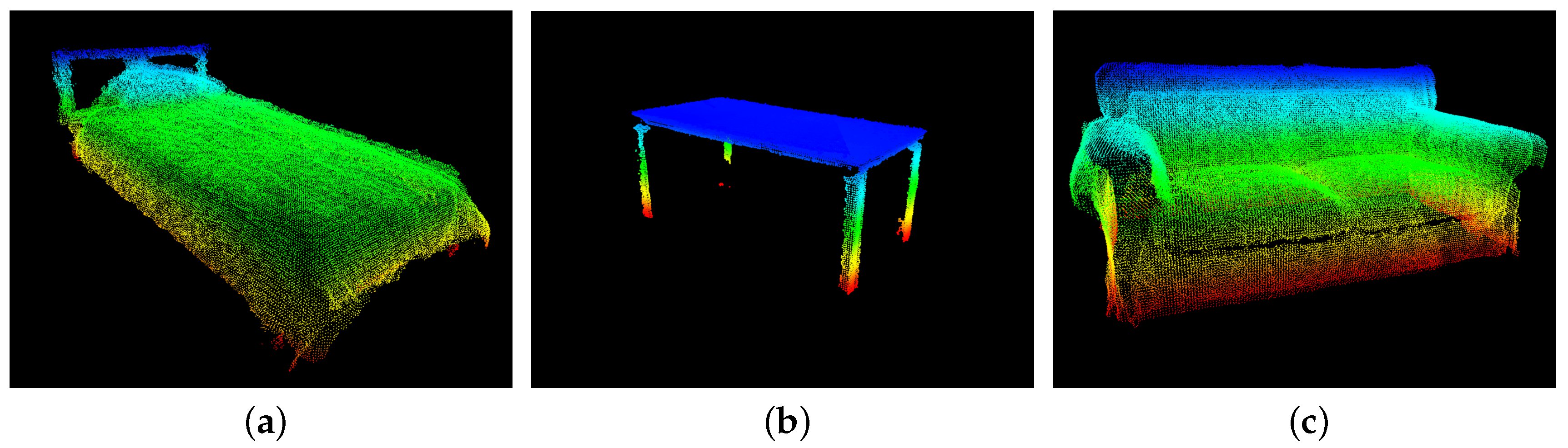
Furniture models were generated from point clouds obtained with an RGB-D camera mounted on the head of the robot, in order to have a similar perception to a human being. The point clouds were merged together with the help of an Iterative Closest Point (ICP) algorithm. In order to make an accurate registration, the ICP algorithm finds and uses the rigid transformation between two point clouds. Finally, a downsample was performed to get an even distribution of the points on the 3D model. This is achieved by dividing the 3D space into voxels and combining the points that lie within into one output point. This allow reducing the number of points in the point cloud while maintaining the characteristics as a whole. Both the ICP and the downsampling algorithm were used from the PCL library [1] In Figure 4, some examples are shown of the 3D point cloud models.

4.1. Extraction of Geometrical Components

Once 3D models of furniture are available, the type of geometric components should be chosen and then extracted. At this stage of the work, it has been decided to use a reduced set of geometrical components, which is composed of horizontal and vertical planes and legs (poles). As can been seen, most of the furniture is composed of flat surfaces (horizontal or vertical) and legs or poles. Conversely, some surfaces are not strictly flat (e.g., the horizontal surface of a bed or the backrest of a coach); however, many of them can be roughly approximated to a flat surface with some relaxed parameters. For example, the main planes for a bed and a table can be approximated by a plane equation, but with different dispersion; a small value for the table and a bigger value for the bed. Currently, curve vertical surfaces have not been considered in our study. Nevertheless, they can be incorporated later.

4.1.1. Horizontal Planes’ Extraction

Horizontal plane detection and extraction is achieved using a method based on histograms. For instance, a table and a bed have differences in their horizontal planes. In order to capture the characteristics of a wide variety of horizontal planes, three specific tasks are performed:

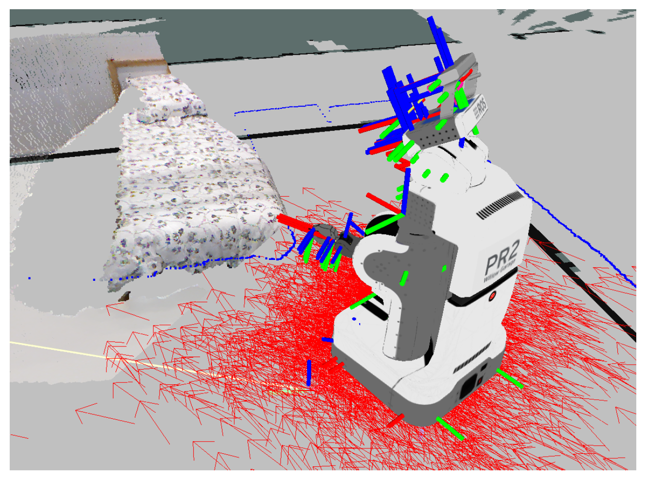
• Considering that a robot and its sensors are correctly linked (i.e., between all reference frames, fixed or mobile), it is possible to obtain a transformation for a point cloud coming from a sensor in the robot’s head into a reference frame to the base or footprint of the robot (see Figure 5). The TF package in ROS (Robotic Operation System) performs this transformation at approximately 100 Hz.
• Once transformation between corresponding references frames is performed, a histogram of heights of the points in the cloud with reference to the floor is constructed.
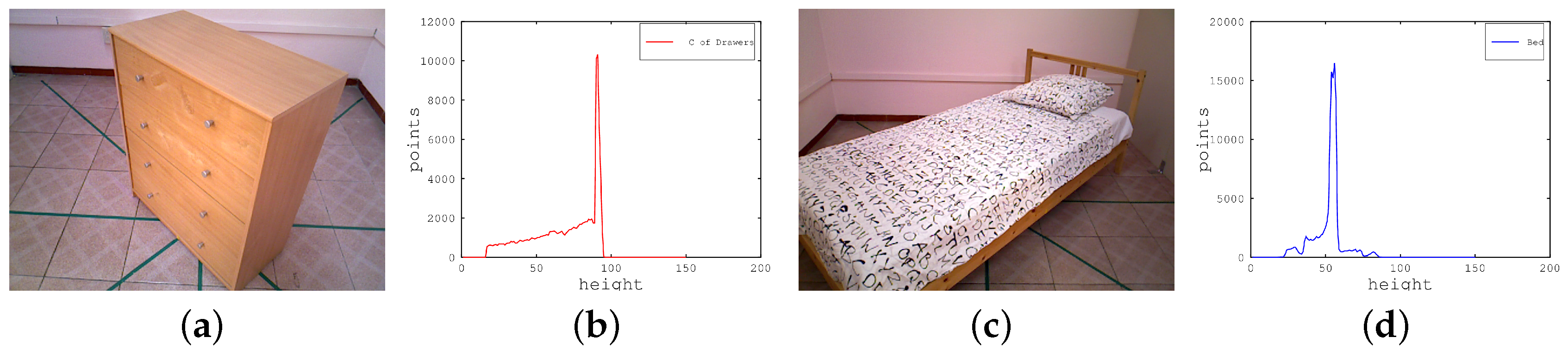
  Over this histogram, horizontal planes (generally composed of a wide set of points) generate a peak or impulse. By extracting all the points that lie over those regions (peaks), the horizontal planes can be recovered. The form and characteristics of the peak or impulse in the histogram refer to the characteristics of the plane. For example, the widths of the peaks in Figure 6 are different; these correspond to: (1) a flat and regular surface for a chest of drawers (Figure 6b) and (2) a rough surface of a bed (Figure 6d).
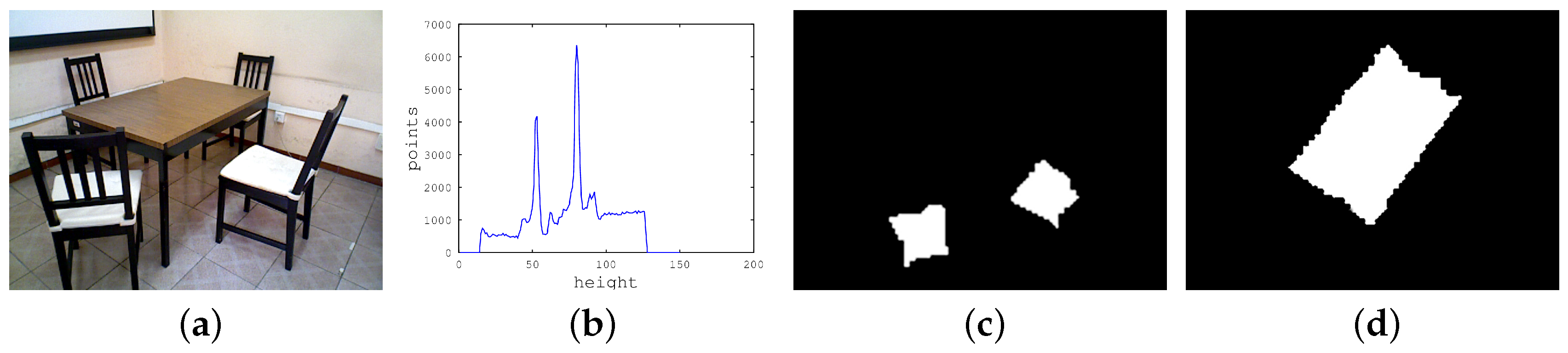
  Nevertheless, there can be several planes merged together in a peak in a scene, i.e., two or more planes with the same height.
• To separate planes merged together in a peak in a scene, first, all the points of the peak are extracted, and then, they are projected to the floor plane. A clustering algorithm is then performed in order to separate points corresponding to each plane, as shown in Figure 7.

4.1.2. Detection of Vertical Planes and Poles

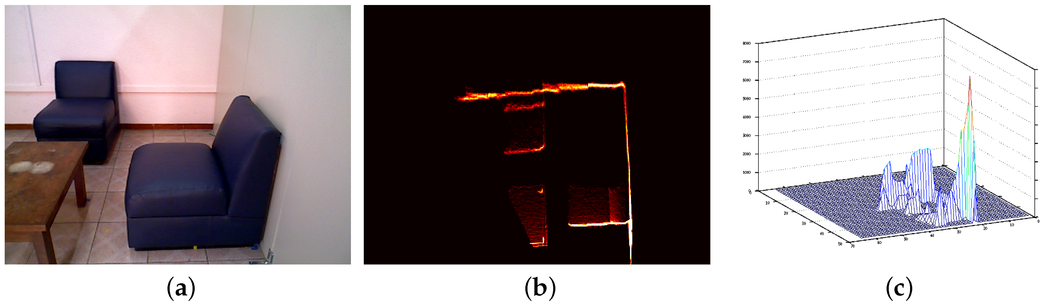
Vertical planes’ and poles’ extraction follows a similar approach. Specifically, they are obtained as follows:

• In these cases, the distribution of the points is analyzed on a 2D histogram generated by projecting all the points into the floor plane.
• Considering this 2D histogram as a grayscale image, all the points from a vertical plane will form a line on the image, and the poles will form a spot; then extracting the lines and spots, and their corresponding projected points, will provide the vertical planes and poles (Figure 8).

Finally, image processing algorithms can be applied in order to segment those lines on the 2D histogram and then recover points corresponding to those vertical planes.

In the cases where two vertical planes are projected to the same line, they can be separated by a similar approach mentioned in the previous section for segmenting horizontal planes; however in this case, the points are projected to a vertical plane. Then, it is possible to cluster them and perform some calculations on them like the area of the projected surface. For the current state of the work, we are more interested in the form of the furniture rather than its parts, so adjacent planes belonging to the same piece of furniture, i.e., the drawers of a chest of drawers, are not separated. If the separation of these planes were necessary, an approach similar to the one proposed in [22] could be used; where they segmented the drawers from a kitchen.

With this approach, it is also possible to detect small regions or dots that correspond to the legs of the chairs or tables. Despite the small sizes of the regions or dots, they are helpful to characterize the furniture.

Our proposal can work with full PCD scenes without any requirement of a downsampling, which must be performed in algorithms like RANSAC in order to maintain a low computational cost. Moreover, histograms are computed linearly.

4.2. Characteristics of the Geometrical Components

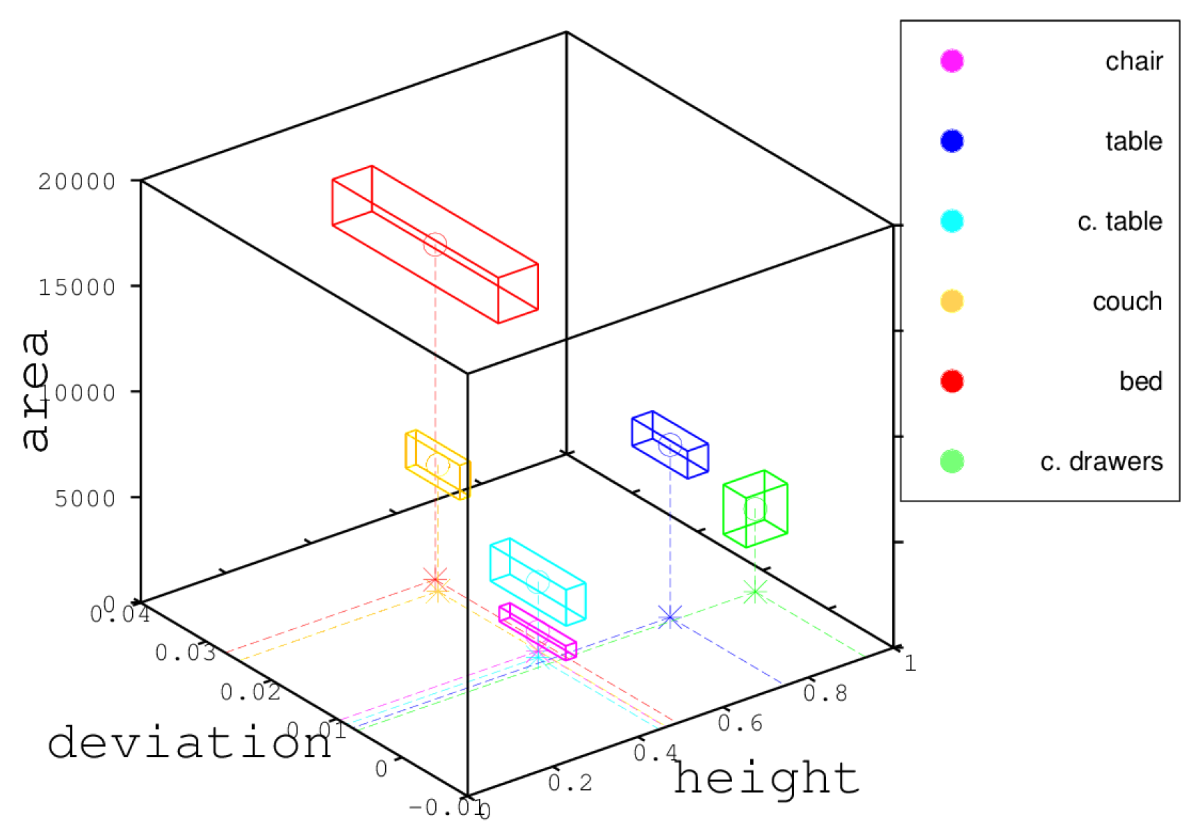
Every geometrical component must be characterized in order to complete the graph for every piece of furniture. For simplicity, at this point, all the geometrical components have the same characteristics. However, more geometrical components can be added or replaced in the future. The following features or characteristics of the geometrical components are considered:

• Height: the average height of the points belonging to the geometric component.
• Height deviation: standard height deviation of the points in the peak or region.
• Area: area covered by the points.

Figure 9 shows the values of each characteristic for the main horizontal plane of some furniture models. The sizes of the boxes were obtained by a min-max method. More details will be given in Section 5.2. The parallelepiped represents the variation (uncertainty) for each variable.

4.3. Examples of Graph Representation

Once geometric components have been described, it is possible to construct a graph for each piece of furniture.

Let $F^{*}$ be a piece of furniture (e.g., a table); therefore, as stated in Equation (1), the graph is described as:

$$\begin{array}{c}\hfill F^{*}=(V^{*},E^{*})\end{array}$$

where $V^{*}$ has five vertices and $E^{*}$ four edges (i.e., $n_v^{*}=5$ and $n_e^{*}=4$). The five vertices correspond to: one vertex for the horizontal surface of the table and one for each of the four legs. The main vertex is the horizontal plane, and an edge will be added whenever two geometrical components are adjacent, so in this particular case, the edges correspond to the union between each leg and the horizontal plane.

Figure 10a presents the graph corresponding to a dinning table. Similarly, Figure 10b shows the graph of a chair. It can be seen that the chair’s graph has one more vertex than the table’s graph. This extra vertex is a vertical component corresponding to the backrest of the chair.

As mentioned earlier, a graph serves as a complete model for each piece of furniture because it contains all its geometrical components. However, as described in Section 3.3, the robot cannot view all the components of a given piece of furniture because of the perspective. Therefore, subgraphs are created in order to compare robot perception with models.

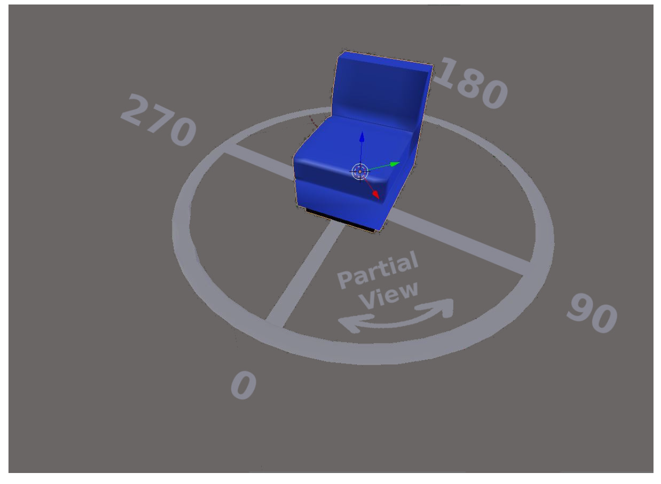
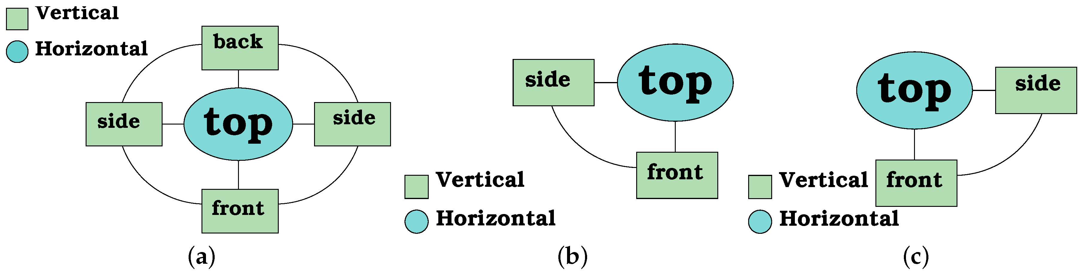
To generate a small set of sub-graphs corresponding to partial views, several points of view have been grouped into four quadrants. These are: two subgraphs for the front left and right views and two more for the back view left and right (Figure 11). However, due to symmetry and occlusions, the set of subgraphs can be reduced. For example, in the case of a dining table, there is only one graph without sub-graphs because its four legs can be seen from many viewpoints.

Consequently, graphs require also to specify which planes are on opposite sides (if there are any), because this information is important to specify which components are visible from every view. The visibility of a given plane is encoded at the vertex. For example, for a chest of drawers, it is not possible to see the front and the back at the same time.

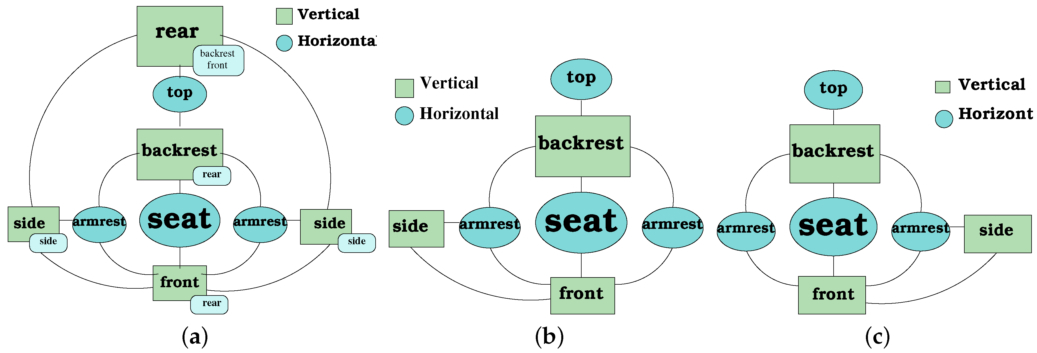
Figure 12 shows an example of a graph model and some subgraphs for a couch graph model. It can be seen from Figure 12a that the small rectangles to the side of the nodes indicate the opposite nodes. The sub-graphs (Figure 12b,c) represent two sub-graphs of the left and right frontal views, respectively. The reduction of the number of vertex of the graph is clear. Specifically, the backrest and the front nodes are shown, whereas the rear node is not presented because it is not visible for the robot from a frontal view of the furniture. Thus, a subgraph avoids comparing components that are not visible from a given viewpoint.

5. Determination of Values for Models and Geometric Components

In order to validate our proposal, a home environment has been used. This environment is composed of six different pieces of furniture ($N_f=6$), which are:

$$\begin{array}{cc}\hfill \mathcal{F}=\{& dinningtable,chair,couch,centertable,\hfill \\ & bed,chestofdrawers\}\hfill \end{array}$$

To represent the components of those pieces of furniture, the following three types of geometrical components have been selected:

$$\begin{array}{c}\hfill \mathcal{G}c=\{horizontalplane,verticalplane,legs\}\end{array}$$

and the features of the geometrical components are described in Section 4.2.

5.1. Weights for the Geometrical Components’ Comparison

In order to compute the proposed similarity $s_{Gc}$ between two geometrical components, it is necessary to determine the corresponding weights $w_{Gi}$ in Equation (6). Those values have been determined empirically, as follows:

From a set of scenes taken by the robot, a set of them where each piece of furniture was totally visible. Then, geometrical components were extracted following the methodology proposed in Section 4.1. The weights were selected according to the importance of each feature to a correct classification of the geometrical component.

Table 1. Weights for similarity estimation.

	${\mathit{w}}_{\mathit{G}1}^{\mathit{k}}$ (Height)	${\mathit{w}}_{\mathit{G}2}^{\mathit{k}}$ (h. Deviation)	${\mathit{w}}_{\mathit{G}3}^{\mathit{k}}$ (Area)
$w_{Gi}^H$ (horizontal)	0.65	0.15	0.25
$w_{Gi}^V$ (vertical)	0.5	0.2	0.3
$w_{Gi}^L$ (legs)	0.5	0.2	0.3

shows the corresponding weights for the three geometrical components.

5.2. Uncertainty

Uncertainty values in Equation (7) were estimated using an empirical process. From some views selected for each piece of furniture fully observable, the difference with its correspondent model was calculated; in order to have an estimation of the variation of corresponding values, with the complete geometrical component. Then, the highest difference for each characteristic was selected as the uncertainty.

As can be seen from Figure 9, the use of characteristics (height, height deviation and area) is sufficient to classify the main horizontal planes. Moreover, over this space, characteristics and uncertainty from each horizontal plane make regions fully classifiable.

There are other features of the geometrical components that are useful to define the type of geometrical component or their relations, so they have been added to the vertex structure. These features are:

• Center: the 3D point center of the points that makes the geometrical component.
• PCA eigenvectors and eigenvalues: eigenvector and eigenvalues resulting from a PCA analysis for the region points.

The center is helpful to establish spatial relations, and the PCA values help to discriminate between vertical planes and poles. By finding and applying an orthogonal transformation, PCA converts a set of possible correlated variables to a set of linearly uncorrelated variables called principal components. Since, in PCA, the first principal component has the largest possible variance, then, in the case of poles, the first component should be aligned with the vertical axis, and the variance of other components should be significantly smaller. This not so in the case of planes, where two first components can have similar variance values. Components are obtained by the eigenvector and eigenvalues from PCA.

5.3. Weights for the Graphs’ Comparison

Conversely, as weights were determined using Equation (7), the weights for the similarity between graphs (Equation (9)) were calculated based on the total area of models for each piece of furniture.

Given the projected area of each geometrical component of the graph model, the total area is calculated. Then, the weights for each vertex (geometrical component) have been defined as the percentage of its area in comparison to the total area. Moreover, when dealing with a subgraph from a model, the total area is determined by the sum of areas from the nodes from that particular view (subgraph). Thus, there is a particular weight vector for each graph and subgraph in the environment.

Table 2. Example of the weights for the comparison of the chest of drawers graph, based on the area of each geometrical component.

	Side	Front	Side	Back	Top
area	1575.5	9155.5	1575.5	9155.5	1914
Model %	6.74	39.16	6.74	39.16	8.19
Partial View %	12.45	72.41			15.13
Partial View %		72.41	12.45		15.13

shows the values of computed areas for the chest of drawers corresponding to the graph and subgraph of the model (Figure 13).

Table 3. Example of the weights for the comparison of the dining table graph, based on the area of each geometrical component.

	Table	Leg	Leg	Leg	Leg
area	8159	947	947	947	947
Model %	68.31	7.92	7.92	7.92	7.92
Partial View %	68.31	7.92	7.92	7.92	7.92

shows the weights in the case of the dinning table, which does not have sub-graphs (Figure 10a).

6. Evaluations

Consider an observation of a scene, where geometrical components have been extracted, by applying the methods described in Section 4.1.

Let O be the set of all geometrical components observed on a scene, then:

$$O=\{O^1,\dots ,O^{N_k}\}$$

(11)

where $O^k$ is the subset of geometrical components of the type k.

In this way, observed horizontal geometrical components found on the scene are in the same subset, lets say $O^{*}$. Consequently, it is possible to extract each one of them in the subset and then compare them to the main nodes for each furniture graph.

Once the similarity between the horizontal components on the scene and the models has been calculated, all the categories with a similarity higher than a certain threshold are chosen as probable models for each horizontal component. A graph is then constructed for each horizontal component, where adjacent geometrical components are merged with it. Then, this graph is compared with the subgraphs of the probable models previously selected.

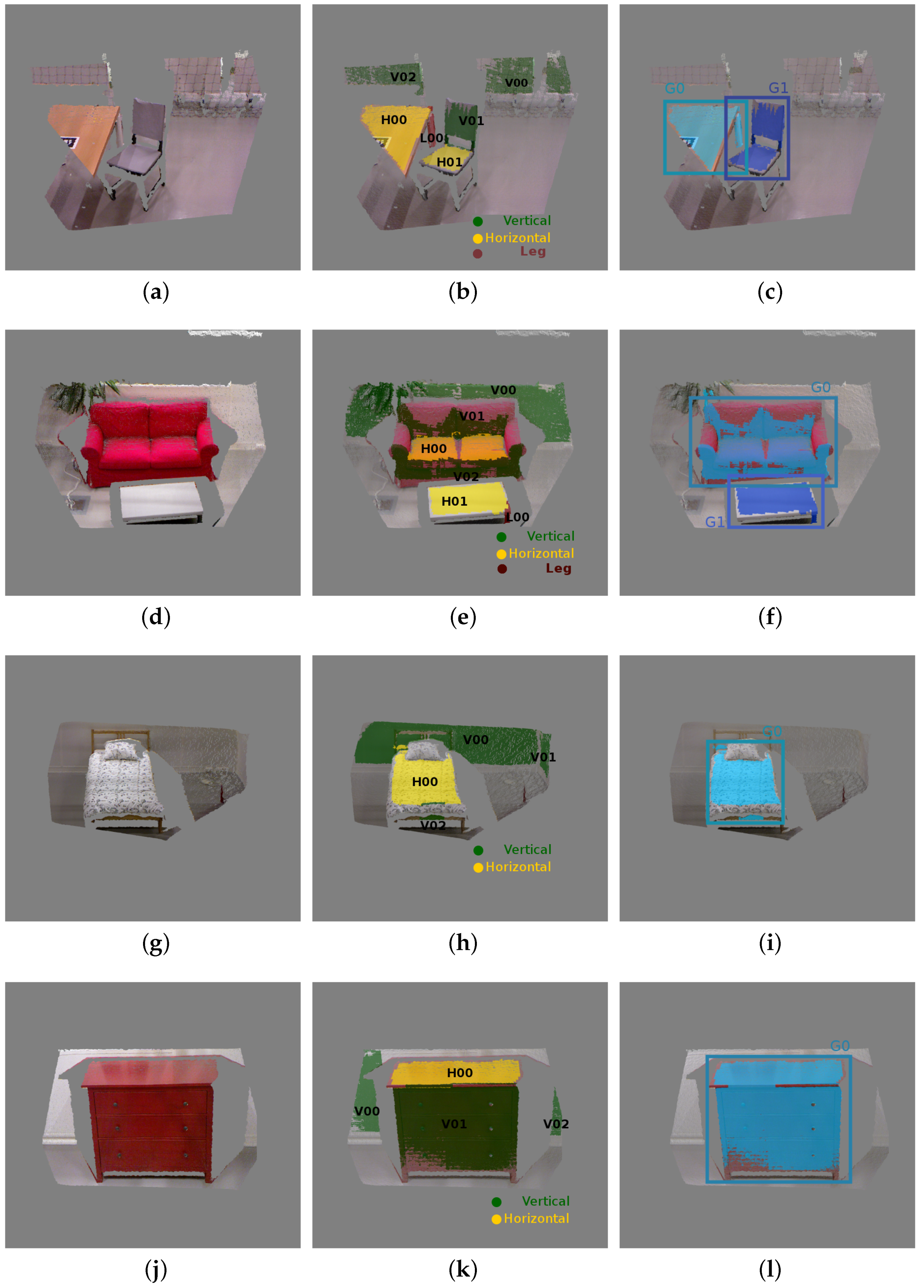
The first column in Figure 14 shows some scenes from the environment, where different pieces of furniture are present. Only four images with the six types of furniture are shown. The scene in Figure 14a is composed of a dinning table and a chair. After the geometrical components are extracted (Figure 14b), two horizontal planes corresponding to the dinning table and the chair are selected.

A comparison of those horizontal components to each one of the main nodes of the furniture graphs is performed. This results in two probable models (table and chest of drawers) for the plane labeled as “H0”, which actually corresponds to the table, and three probable models (chair, center table and couch) for the plane labeled “H01” (which corresponds to a chair). The similarities computed can be observed as “Node Sim.” in

Table 4. Example for graph classification.

Main Node	Main Node Sim.	Adjacent Nodes	Adjacent Node Sim.	Graph Similarity
H00	Table	V02	Table leg	0.0.6670
	0.8743		0.7015
H00	Chest of Drawers	V02	No Match	X
	0.8014
H01	Chair	V01	Backrest	0.5740
	0.9891		0.8878
H01	Center Table	V01	No match	X
	0.8895
H01	Couch	V01	Backrest	0.3204
	0.7277		0.7150

.

Next, graphs are constructed for each horizontal plane (the main node) and adding its adjacent components. In this case, both graphs have only one adjacent node.

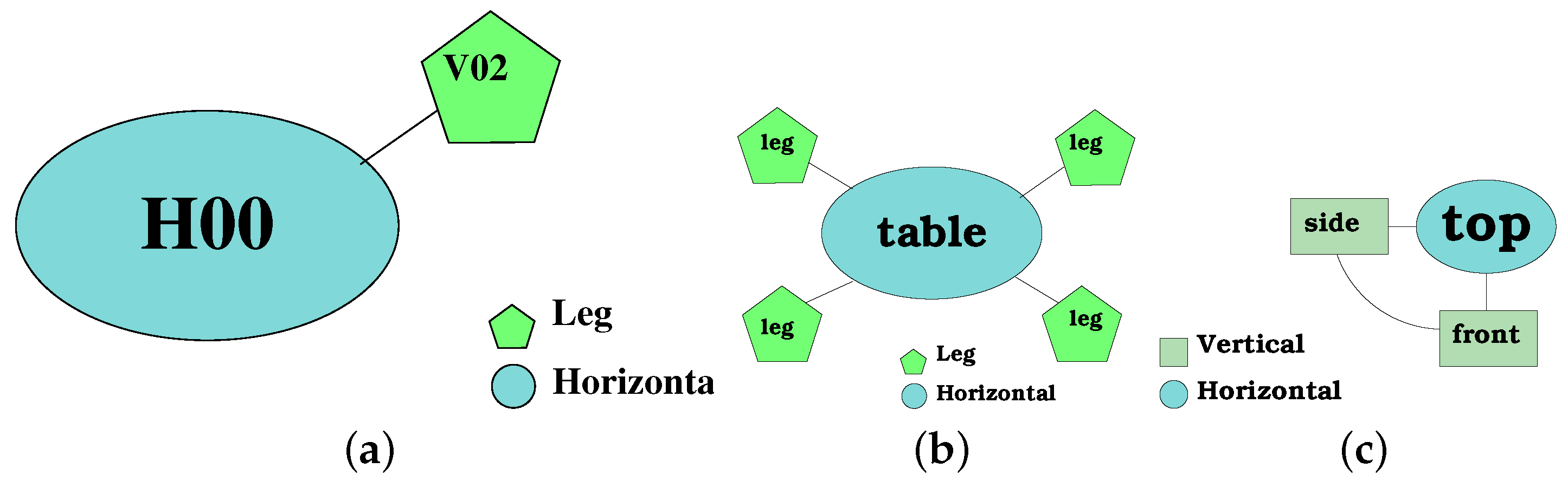
Figure 15a shows the generated Graph (“G0”) from the scene and the partial-views graphs from the selected probable models. It can be observed that “G0” has an adjacent leg node, so it can only be a sub-graph for the table graph since the chest of drawers graph has only adjacent vertical nodes.

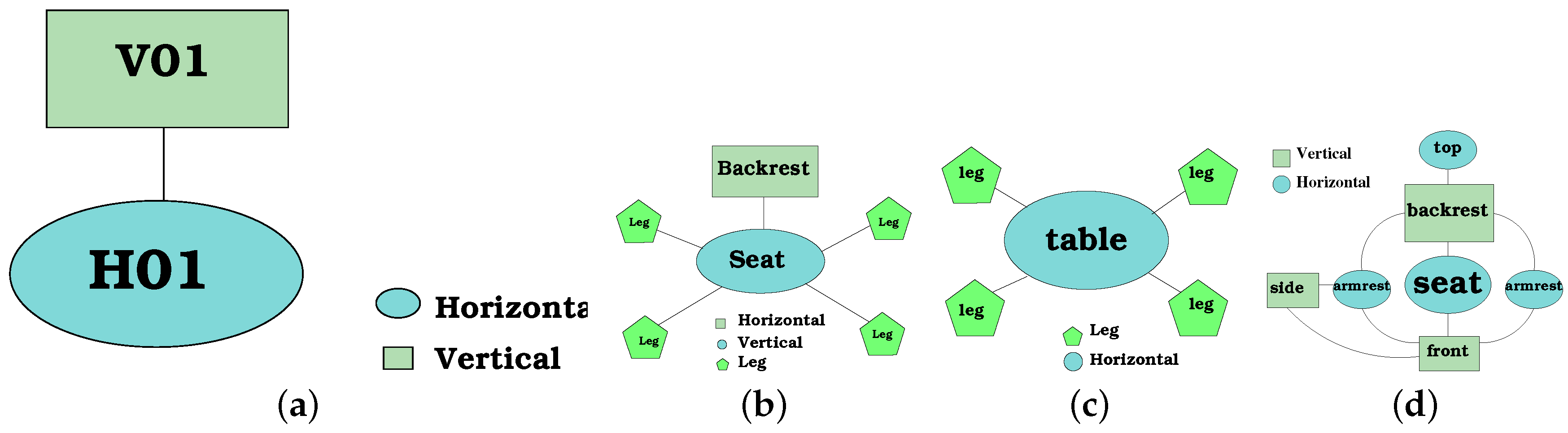
For “G1” (Figure 16a), its adjacent node is a vertical node with a higher height than the main node, so it is matched to the backrest node of the chair and of the couch (Figure 16b,d). Moreover, there is no match with the center table graph (Figure 16c).

The similarity for adjacent nodes is noted in Table 4. Graph similarity is calculated with Equation (9) and shown in the last column of the table. “G0” is selected as a table and “G1” as a chair (Figure 14c).

Figure 14 shows the results of applying the described procedure to different scenes with different types of furniture. The first column (Figure 14a,d,g,j) shows the point clouds from the scenes. The column at the center (Figure 14b,e,h,k) shows the geometrical components found on the corresponding scene. Finally, the last column (Figure 14c,f,i,l) shows the generated graphs classified correctly.

As our approach is probabilistic, it can deal with the noise from the sensor; as well as partially occluded views, at this time, with occlusions no greater than 50% of the main horizontal plane, as this plane is the key factor in the graph.

While types of furniture can have the same graph structure, values in their components are particular for a given instance. Therefore, it is not possible to recognize with the same graph different instances of a type of furniture. In other words, a particular graph for a bed cannot be used for beds with different sizes; however, the graph structure could be the same.

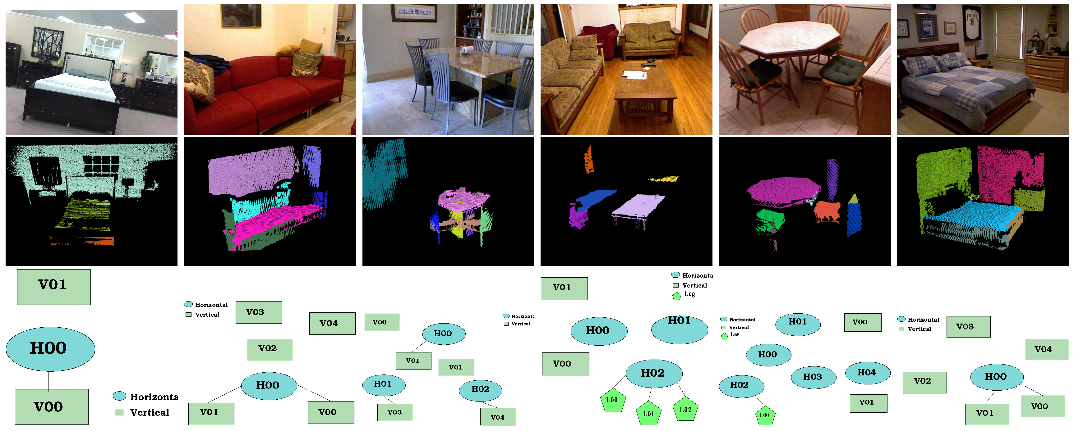
Additionally, to test the approach on more examples, we have tested on selected images from the dataset SUNRGB-D [23]. Figure 17 shows the results of the geometrical components’ extraction and the graph generation for the selected images. The color images corresponding to house environments similar to the test environments scenes are presented at the top of the figure; the corresponding geometrical component extraction is shown at the center of the figure; and the corresponding graphs are presented at the bottom of the figure.

It is important to note that to detect the geometrical components over these scenes, the point cloud from each selected scene was treated using the intrinsic and extrinsic parameters provided in the dataset. Consequently, a similar footprint reference frame is obtained such as the frame provided by the robots in this work. This manual adjustment was necessary to simulate the translation needed to align the coordinate frame of the image with the environment, as described in Section 4.1.

Since the proposed approach requires a complete model for each piece of furniture, which were not provided by the dataset, it was not possible to match the graphs generated to a given piece of furniture. However, the approach has worked as expected (Figure 17).

7. Conclusions and Future Work

This study proposed a graph representation useful for detecting and recognizing furniture using autonomous mobile robots. These graphs are composed of geometrical components, where each geometrical component corresponds roughly to a different part of a given piece of furniture. At this stage of our proposal, only three different types of geometrical components were considered; horizontal planes, vertical planes and the poles. A fast and linear method for extraction of geometrical components has been presented to deal with 3D data from the scenes. Additionally, similarity metrics have been proposed in order to compare the geometrical components and the graphs between the models in the learned set and the scenes. Our graph representation allows performing a directed search when comparing the graphs. To validate our approach, evaluations were performed on house-like environments.

Two different environments were tested with two different robots provided with different brands of RGB-D cameras. The environments presented the same type of furniture, but not completely the same instances; and robots had their RGB-D camera in the head to provide a similar point of view to a human. These preliminary evaluations have proven the efficiency of the presented approach.

As future work, other geometrical components (spheres and cylinders) and other characteristics will be added and assessed to improve our proposal. Furthermore, other types of furniture will be evaluated using our proposal.

It will be desirable to bring the robots to a real house environment to test their performance.