Minimum Barrier Distance-Based Object Descriptor for Visual Tracking

School of Computer Science and Technology, Anhui University, Hefei 230601, China
*
Author to whom correspondence should be addressed.
Appl. Sci. 2018, 8(11), 2233; https://doi.org/10.3390/app8112233
Submission received: 10 September 2018
/
Revised: 24 October 2018
/
Accepted: 30 October 2018
/
Published: 13 November 2018
(This article belongs to the Special Issue Advanced Intelligent Imaging Technology)
Abstract
:In most visual tracking tasks, the target is tracked by a bounding box given in the first frame. The complexity and redundancy of background information in the bounding box inevitably exist and affect tracking performance. To alleviate the influence of background, we propose a robust object descriptor for visual tracking in this paper. First, we decompose the bounding box into non-overlapping patches and extract the color and gradient histograms features for each patch. Second, we adopt the minimum barrier distance (MBD) to calculate patch weights. Specifically, we consider the boundary patches as the background seeds and calculate the MBD from each patch to the seed set as the weight of each patch since the weight calculated by MBD can represent the difference between each patch and the background more effectively. Finally, we impose the weight on the extracted feature to get the descriptor of each patch and then incorporate our MBD-based descriptor into the structured support vector machine algorithm for tracking. Experiments on two benchmark datasets demonstrate the effectiveness of the proposed approach.
1. Introduction
Object tracking is an important issue for video analysis in the field of computer vision, with wide-ranging applications including surveillance, human-computer interaction and medical imaging. Given the first frame including the target location and the size of the bounding box, the object tracking task is to estimate the location of the target in the current frame without the target motion information in advance [1]. In recent years, along with many new tracking algorithms emerging, the performance of visual tracking has been greatly promoted. However, object tracking is still a challenging issue due to many problems existing in the tracking process such as illumination variation, occlusion, large deformations and background clutters, which are not solved well. Therefore, object tracking still needs to be investigated. In this paper, we tackle the complex background challenges in the bounding box caused by target occlusion, large deformations or background clutters in visual tracking.
As an important branch in visual tracking, many tracking-by-detection algorithms [2,3,4,5,6,7,8,9] have attracted much attention. The idea of tracking-by-detection algorithms is regarded as finding target localization as a classification problem. The classifier is trained with positive and negative samples corresponding to foreground and background areas, respectively. During the tracking process, the object always has occlusion, deformation or size variation, leading to the bounding box containing too much background area, which brings a negative influence to the classifier updating. To reduce the effect of an enlarged background, a new representation for the target was proposed, called the spatially-ordered and weighted patch descriptor (SOWP) [10], which conveys structural information of the object within the bounding box. However, SOWP uses a calculation method similar to Euclidean distance to calculate the similarity between two patches, as well as many current tracking algorithms [6,11,12,13], which makes it difficult to distinguish the target from the background when there are some appearance similarities brought by background blur, occlusion or fast motion in the bounding box.
In order to improve the above problem and considering that the minimum barrier distance (MBD) [14] is more robust to pixel value fluctuation caused by motion or noise, we construct a robust object representation by applying MBD to calculate the weights of patches. Given the bounding box of a target in the search area, we divide it into non-overlapping patches and describe them with a combination of an RGB (Red-Green-Blue) color histogram and a histogram of oriented gradients (HOG) feature. Then, we expand the bounding box outwards, and the boundary patches in the extended bounding box are regarded as the seed patches according to the appearance-based backgroundness cue [15,16]. The image boundary prior assumes that most of the image boundary area is background [15], so we set the boundary patches as the background seed set. Instead of generating an affinity matrix by calculating the similarity between patches, we construct the MBD-based descriptor through a distance transform map for visual tracking. Specifically speaking, we use each patch as a node and two adjacent nodes to form an edge and obtain a distance transform map by iteratively calculating the MBD from each patch to the seed set. The weight of each node represented by the value of the MBD describes how likely this patch belongs to the target. The larger the value of the MBD, the smaller the similarity of the current patch to the boundary patch and the greater the probability that the current patch belongs to the target.
As shown in Figure 1, the target in the sequence “Skating2-1” is a female skater, and it is obvious that the video includes fast motion and deformation due to the rapid movement of the skater. The bounding box in the result of SOWP [10] and contains a large number of background regions (male skaters) in Frame 136, resulting in false tracking and the loss of real targets at Frame 396. The athletes in the sequence “Bolt2” are almost similar to each other in appearance, and their appearance changes significantly due to background clutter and deformation, which leads to SOWP [10], ACFN (Attentional Correlation Filter Network) [18] and MEEM (Multiple Experts Using Entropy Minimization) [19] mistakenly tracking other athletes; meanwhile, the trackers MUSTer (MUlti-Store Tracker) [20] and TLD (Tracking-Learning-Detection) [21] drift. It is easy to see that our algorithm achieves accurate tracking under these challenges because MBD is used for calculating the similarity between the target and the background.
The main contribution of this paper is that we present a novel MBD-based descriptor for visual tracking. Specifically, we propose to apply the MBD to calculate the weights of patches to construct the object descriptor for visual tracking, since MBD is more robust to pixel value fluctuation caused by motion or noise. Then, we adopt the boundary patches on each side in the bounding box as labeled background queries and calculate the MBD between the image patches and the seed patches; thus, the foreground target can be highlighted, and the background noise can be suppressed. Extensive experiments demonstrate that our proposed MBD-based descriptors can achieve more robust performances against other recent visual trackers when confronting fast motion and background clutter, as well as reduce drift effectively.
The rest of this paper is organized as follows: Section 2 reviews the background and some state-of-the-art or classic methods related to our method. We will give a detailed introduction of our proposed algorithm in Section 3. Section 4 discusses experimental results including qualitative analysis and quantitative analysis. We draw the conclusion of this paper in Section 5.
2. Related Work
Visual tracking is an important issue in computer vision, as it is the foundation of a high level visual task. The current tracking algorithms can be divided into two major categories: generative models [22,23,24,25] and discriminative models [26,27,28,29,30,31]. By describing the target appearances using generative models such as subspace models, generative methods search for regions most similar to the target object and updating the appearance model dynamically to solve object tracking. In general, the generative models focus on the characterization of the target and ignore the background information; hence, they are prone to drift when the target changes dramatically and often fail in a cluttered background [21]. In contrast, discriminative trackers build a binary classifier, which focuses on differentiating the target from the background [32]. Belonging to discriminative trackers, adaptive tracking-by-detection approaches build a classifier during tracking and update the classifier using generated binary labeled training samples around the current object location [21]. To avoid the label errors during the classification step, the kernelized structured output support vector machine (SVM) has been used in [33] for adaptive visual object tracking. However, this method uses simple low-level features and has low efficiency at handling occlusion. Therefore, generating correct labeled training samples is very important for the classifier updating, and designing a good sample descriptor is crucial for distinguishing positive or negative samples clearly.
As we mentioned above, tracking-by-detection approaches almost perform not well when there is complex background information in the bounding box, which inevitably exists, caused by occlusion, deformation, size variation and background clutters. Many works have been proposed to improve the robustness of trackers to handle the influence of these challenging problems. Lu et al. [34] proposed a pixel-wise appearance model called pixel-wise spatial pyramid, which employs the pixel feature vector to combine several features. This pixel-wise spatial pyramid contributes to the accurate location of the tracked object, especially for drastic appearance change. Wei et al. [35] proposed a locality sensitive histogram, taking into account the contributions from each pixel and facilitating robust multi-region tracking. However, these pixel-based trackers failed to handle occlusion and cluttered background due to pixel-wise appearance models lacking structural information.
For improving some pixel-based trackers, superpixel-based trackers [36,37,38] then came out to handle non-rigid and deformable targets, by segmenting images into superpixels and providing the semantic structure of the target. Wang and Yang et al. [36,39] built the superpixel-based appearance models, with some effects on object occlusion and deformation. However, trackers based on superpixels are complex and have difficulty dealing with cluttered backgrounds, which often lead to unstable results. In recent years, patch-based tracking methods have received more attention, because patch-based trackers can describe the structure information of the object better, and they often use different descriptors to represent the object [10,12,40]. As a new and effective method, SOWP [10] decomposed the object bounding box into multiple patches, and the patch weights were calculated by performing random walk with restart simulations. The weighted patch descriptor [10] is more flexible for partial occlusion and appearance changes of the object. Similar to SOWP, some methods [41,42] weight the sample with patch likelihoods in particle filters, and [43] used adaptive weighting in patch-based correlation filters to mitigate the effect of occlusion. However, when the object is occluded for a long time, SOWP still has drift, and it is difficult to distinguish target and background when there are some appearance similarities brought by background blur or target occlusion in the bounding box. In this paper, we propose a novel approach to solve the appearance similarity measure problem by minimum barrier distance weighting. Experiments have shown that the performance of our method has a better robustness than many other visual trackers.
3. The Proposed Algorithm
3.1. Overview
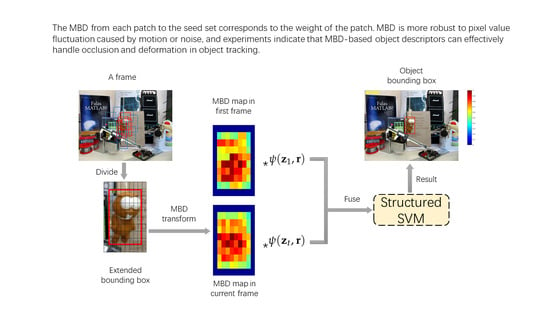
We propose a novel tracking algorithm named the MBD-based descriptor for tracking. Given a candidate bounding box of a target in a search region at the current frame, we first divide it into patches and expand the bounding box to patches, as shown in Figure 2b. Each patch is described with a combination of RGB color histogram and HOG feature. Then, in each frame, an MBD map is constructed for each bounding box, and we calculate the MBD from each patch to the seed set, which is represented as S, and generate an MBD transform map by performing the raster scan, as well as the MBD of each patch corresponding to the weight of the patch, which reflects the difference between target and background. Finally, we combine MBD with corresponding patch features to construct a robust object descriptor and evaluate the descriptor on structured SVM to carry out the tracking. The pipeline of our algorithm is shown in Figure 2.
3.2. Patch-Based Representation
First, we divide the bounding box into patches, and different gridding sizes from to are tried in the proposed method. We decided to divide the bounding box into 64 patches as a trade-off between accuracy and efficiency, i.e., the parameter n is 8. Since the results will become worse if adopting other gridding sizes bigger or smaller than 8 ∗ 8, a patch should have the proper size to make the tracker more robust. Each patch is characterized with a d-dimensional feature vector through a combination of the RGB color histogram and HOG feature. Then, the feature descriptor [10] for a bounding box in the t-th frame is given by:
where represents a bounding box in the t-th frame and is the feature vector of each patch. is a simple feature descriptor for . To assign a weight for each patch, we adopt the MBD to calculate it. By considering these patches as nodes V and the 4-neighbor links between patches as edges E, the bounding box in the current frame can be represented by a graph . The MBD from a patch to seed set S reflects the difference between the patch with background. Therefore, our next step is to calculate the MBD between each patch and the boundary patches, while the MBD of each boundary patch is set to 0. Then, the distance is regarded as the weight of each patch, which describes how likely it belongs to the target object.
3.3. MBD-Based Patch Weighting
The MBD is defined by the path cost function. It is the minimum value of the barrier strength of the path between two nodes in the path [14]. The difference between MBD and a common distance function is that the length of the path may remain constant during the growth of the path, until a new, stronger barrier is encountered on the path. The MBD calculates the distance value in a digital image effectively. MBD has many interesting theoretical properties. It has proven to be a potentially useful tool in image processing [44]. When considering the variation of the seed position and the introduction of noise, it is advantageous compared to fuzzy and geodesic distance [45].
In the graph , we set , where represents patch i. Then, a path on the graph refers to a sequence of patches along a to c, and this sequence contains any path , where and are adjacent , i∈ {}. We use to denote all the paths connecting the seeds to c, and indicates the path cost on the path . Then, we calculate the distance for node c to the seeds and update the distance map with the following formula:
The definition of the function f depends on the image intensity and differs for different methods. In our work, to calculate the barrier distance, we use to denote the path cost connecting S to node i on graph G, and the cost function of distance transform [46] is defined as:
where returns the MBD of path , which is the formula for the MBD transform. Similar to the raster scan algorithm used for the geodesic distance transform [46], we need to access each patch in the raster scan or reverse raster scan in order. In the raster scan method, the distance values are propagated by sequentially scanning the image in a predefined sequence. That is, each line is scanned, first from the upper left to the lower right, and then from the lower right to the upper left until convergence (see the illustration in Figure 3). For example, when visiting a node x in a raster scan order, for each node b in the mask area of the current node x as shown in Figure 3b, we compute the MBD of x according to Equation (4).
where and represent the highest and lowest values on b, respectively, which are used to ensure the highest and lowest values of the cost on the current path, and H and L are auxiliary maps. Given the image G, the seed set S is set to 0, and is initialized to ∞. refers to the path cost of MBD for each path from the node x to S. Then, the distance map D and the auxiliary maps are updated in a raster scan pass and an inverse raster scan pass, until the number of iterations is k. The MBD is updated when the value of path costs is greater than the current maximum or less than the current minimum in the path [46,47].
where refers to the path from x to S, b is the adjacent node of x and represents the path from the node x to S and through the node b. For example, a path connects the node b to the seed set S, and the edge is appended to the path to form a new edge, which is denoted as , each adjacent node b of x is used to minimize x iteratively. If , update to . Meanwhile, update to max{, }, to min{, }, and then, visit the next node. We summarize the MBD transform in Algorithm 1, and k is the number of iterations in the raster scan.
As shown in Figure 3, one raster scan will only access the two neighbors of the current node since graph G is a map of the 4-neighbor. indicated by the green arrow represents a path from current node x to S and through its upper neighbor , and represents the path of the current node to S and through its left neighbor ; if , then .
Finally, we can obtain the enhanced object descriptor by multiplying the feature descriptor with the corresponding patch weight as follows:
| Algorithm 1 Minimum Barrier Distance transform. |
| Input: image G, seed set S, number of passes k. Output: MBD map D.
|
3.4. Structured SVM Tracking
In this section, we incorporate our descriptor into the conventional tracking algorithm, structured SVM [4], as Struck [4] excels in the recent benchmark according to [1,10]. Firstly, we set a searching window around the bounding box obtained in the previous frame. Then, in the searching window, our MBD-based descriptors for candidate bounding boxes are incorporated into structured SVM to estimate the maximum classification score and select the current bounding box standing for the object. Finally, we may need to update the classifier and proceed to the next frame. Specifically, Struck estimates the object bounding box in the t-th frame by maximizing a classification score. To avoid the model drift, we fuse the model of the first frame and the current frame in our algorithm. The bounding box , which can maximize a classifier score, is the object, as follows:
where is the normal vector of a decision plane and is learned in the initial frame. represents the weighted feature descriptor for bounding box in frame t, and is a tradeoff parameter. Maximizing a classifier score by evaluating the samples represented with weighted features can obtain the best classification.
We adopt the good strategy mentioned in SOWP [10] to detect abrupt changes of object appearance, and we update the classifier when the confidence score of the tracking result is greater than a threshold . A confidence score is given by:
where s is a positive support vector and is the set of s at time t. The confidence score in the t-th frame refers to the average similarity between the MBD descriptor of the tracked bounding box and the positive support vectors. Therefore, the confidence score measures the reliability of the object in the bounding box in the current frame.
We estimate the target scale by training a scale classifier on a scale pyramid [48]. This allows us to estimate the target scale independently after the optimal position is found. stands for the object size in the current frame, and M is the size of the scale filter. Then, we extract an image patch with the size centered around the target as follows:
4. Experimental Results
The proposed tracker with MBD-based descriptor was implemented in C++ on an Intel Core i7-6700K (Intel Corporation, Santa Clara, CA, USA) 3.40 GHz CPU with 8 GB RAM and run at 4.7 FPS (frames per second). We evaluated our tracker on the OTB-100 (object tracking benchmark) dataset [17] and TColor-128 (Temple Color) dataset [49]. The experimental results demonstrate the effectiveness of our algorithm through qualitative analysis and quantitative analysis. For a fair comparison, the parameter was empirically set as 0.395, and a = 1.052, M = 33, = 0.3, k = 3 for all the sequences in the experiment.
4.1. Evaluation Method
We evaluated our tracker on the OTB-100 dataset [17] and TColor-128 dataset [49]. In these datasets, precision rate (PR) and success rate (SR) were adopted to evaluate the quantitative performances of trackers. The precision shows the ratio of frames that the distance between the estimated bounding box and the given ground-truth is smaller than a threshold. OTB-100 uses the score when the threshold is set to 20 pixels as the representative precision rate score for each tracker. By measuring the overlap ratio between the estimated bounding box and ground-truth, success rate counts the number of successful frames whose overlap ratio is larger than the given threshold 0.5. The area under curve (AUC) of each success plot is adopted to rank the tracking algorithms.
4.2. Qualitative Evaluation
We will first perform the qualitative analysis. Comparing with SOWP [10], we found that our algorithm can track the target accurately in many challenging sequences, while the SOWP failed. As shown in Figure 4, the “Basketball”, “Car4”, “Freeman1”, “Girl2”, “Lemming”, “Suv” and “Human3” sequences contain occlusion, background clutters, scale variation and deformation, for which many trackers cannot track the given object accurately. In this work, we compare our tracker with SOWP on OTB-100 and give some results in Figure 4. The illustration shows that the proposed approach effectively handled scenes’ fast motion (“Basketball” and “Lemming”), background clutters (“Car4” and “Basketball”), occlusion (“Freeman1”, “Suv” and “Human3”) and deformation (“Basketball”, “Girl2” and “Human3”). For example, SOWP lost the object on the sequence “Basketball”, due to sudden illumination variation and another athlete with a similar appearance. In contrast, our tracker could track the target successfully. SOWP also did not perform well on the sequence “Lemming”. When the object reappeared in frame 901, SOWP failed to find it, but our tracker could track it steadily. The performance of SOWP was not satisfactory for sequence "Freeman1" due to background blur. It considered some background as a part of the target and led to inaccurate tracking results. It is easy to find that our algorithm could achieve better results on these challenging videos due to the utilization of weighted patches with the MBD.
4.3. Quantitative Evaluation
4.3.1. Evaluation on OTB-100
OTB-100 includes 100 video sequences with fully-annotated ground-truth and attributes. It groups 100 sequences into 11 different attributes, including illumination variation (IV), out-of-plane rotation (OPR), scale variation (SV), occlusion (OCC), deformation (DEF), motion blur (MB), fast motion (FM), in-plane rotation (IPR), out-of-view (OV), background clutters (BC) and low resolution (LR). In addition to the 29 trackers given by OTB-100, we also compared the proposed algorithm with some recent proposed tracking methods, and Table 1 shows the results of a comparison between our tracker and nine recent trackers, including SOWP [10], ACFN [18], MEEM [19], MUSTer [20], LCT (Long-term correlation tracking) [50], DSST (Discriminative Scale Space Tracker) [48], KCF (Kernelized Correlation Filters) [5], Struck [4] and TLD [21], among which ACFN [18] is a deep learning method. We used the PR/SR scores proposed in OTB-100, and the results of the trackers were obtained by running the published codes. We found that our tracker performed not well especially for the low resolution (LR) sequences, as shown in Table 1, because our algorithm took boundary patches as seeds in the bounding box, and the low resolution or heavy background clutter would influence the initialization of seeds, which led to unsatisfactory results in these cases. However, we observed that our tracker performed favorably against the other state-of-the-art trackers, and it achieved the best overall performance and performed well in most of the attributes.
In order to evaluate the effectiveness of the proposed MBD-based object descriptor, we compared our algorithm with recent trackers and replaced the MBD with different distance metrics in Table 2. The results in Table 2 indicate that our algorithm performed well compared to several state-of-the-art algorithms including MemTrack (Dynamic Memory Networks) [51], scaleDLSSVM (Dual Linear Structured SVM) [29], DCFNet (Discriminant Correlation Filters Network) [52], CNN-SVM (Convolutional Neural Network) [8], SiamFC-3s (Fully-Convolutional Siamese Networks) [53] and SINT++ (Siamese Network) [2]. Of these trackers, MemTrack [51] and SINT++ [2] are neural network-based methods; scaleDLSSVM [29] and CNN-SVM [8] are tracking-by-detection-based methods; DCFNet [52] and SiamFC-3s [53] are correlation filter-based methods. In addition to the latest tracker MemTrack, which obtained comparable results to ours, our method was better than other state-of-the-art algorithms. OURS-Eu, OURS-L1 and OURS-KL are the results of replacing our MBD with Euclidean distance, L1 distance and KL divergence, respectively. To verify the effectiveness of MBD-tuned weights, we also created a version of our algorithm with random weights subjected to Gaussian distribution, named OURS-Ga. Our method also gets better results than OURS-Eu, OURS-L1, OURS-KL and OURS-Ga, which verifies the effectiveness of MBD-tuned weighting.
We rank the top 16 trackers by running the one-pass evaluation (OPE) on the OTB-100 as shown in Figure 5. MemTrack [51] is the latest method based on a deep network and obtained comparable results to ours. Our tracker (0.835/0.595) achieved performance gains of in precision and in success rates over MEEM [19] (0.781/0.530), even if MEEM may have recovered from the corrupted classifier by utilizing a multi-expert tracking framework. Our tracker outperformed the tracker SOWP [10] (0.803/0.560) with in precision and success rates, respectively. That means that our method had a more robust descriptor than SOWP, which also used patch descriptors.
We present the precision plots and success plots with eight different attributes in Figure 6 such as DEF, OPR, SV, OCC, OV, MB, FM and BC. We can see from the illustration that our algorithm outperformed on deformation compared with other trackers; especially, our tracker was better than the second tracker CNN-SVM [8] by and in precision and success rates on DEF, respectively. At the same time, our tracker achieved performance gains of in the PR score and in the SR score over SOWP [10] on FM. Compared with SOWP adopting the weighted descriptor, it shows that the MBD-based weighted patches performed more robustly with the fluctuation of node values.
The results in Figure 6 show that the hard positive sample generated by training the hard positive transformation network in SINT++ [2] was advantageous for OV, while our methods outperformed SINT++ in the other seven attributes. The latest MemTrack [51] obtained the best results on most of the attributes due to the superiority of deep networks. The MUSTer [20] tracker achieved better results over ours for BC by exploiting both the short-term and long-term systems to process the image with the target being tracked, but its overall performance was not so robust as ours. ACFN [18] achieved better results for SV in the success plots than our method, but our algorithm outperformed against the ACFN on the other attributes including OCC, FM and BC. This shows that our proposed MBD-based weighted descriptor could locate the target object in a complex background even without strong features. These experiments validate the effectiveness of the proposed algorithm.
We compared our tracker with real-time part-based visual tracking (RPVT) [43] with dynamic weighting. RPVT tested its method on 16 selected challenging tracking sequences in OTB-50 [1] to show its ability for handling occlusion, scale and appearance changes. We have also run our method on the same sequences and adopted the average center location error and average overlap rate the same as in that paper, and the results are shown in Table 3 and Table 4. In general, RPVT obtained better results than ours for these 16 tracking sequences. However, our tracker performed better on the most of the other 34 sequences in Table 5. This evinces that RPVT was better for handling occlusion, scale and appearance changes, while our tracker was good at the challenges including fast motion, background clutter and deformation.
We also compared our tracker with the occlusion probability mask-based tracker (OPM) [41]. We ran our method on the same sequences and adopted the same average center location error for comparing with this method, and the results are shown in Table 6. OPM selected eight sequences from OTB-100 in its experiment. We can see from Table 6 that OPM performed better than ours on these sequences, and this shows that OPM had advantages in dealing with some sequences with occlusion; however, our tracker performed better for the sequences with illumination variation and scale variation.
4.3.2. Evaluation on TColor-128
TColor-128 [49] contains a large set of 129 color sequences with ground truth and challenge factor annotations. Compared with OTB-100, TColor-128 contains more challenging sequences and is more difficult to track. We evaluated our tracker on the TColor-128 dataset and show the evaluation results between our tracker and recent trackers including Staple [54], DGT (Dynamic Graph for Visual Tracking) [9], MEEM [19], Struck [4], KCF [5], ALSA ( Adaptive Structural Local Sparse Appearance Model) [55] and LCT [50] in Figure 7.
4.3.3. Evaluation on Challenges
Occlusion is a difficult issue as the object might be occluded by other objects or disappear from the scene. Inspired by [56,57], we evaluated the proposed algorithm on motion blur and different levels of occlusion and background clutter, as shown in Table 7. We divided these challenges into partial occlusion (PO) [57], heavy occlusion (HO) [57], slight background clutter (SBC), heavy background clutter (HBC), motion blur (MB) and deformation (DEF). We have found 84 sequences in total with occlusion in OTB-100 and TColor-128 datasets, including 41 partial occlusion and 43 heavy occlusion sequences. Almost all the targets in these sequences with heavy occlusion were completely occluded and disappeared. We also found 31 sequences with slight background clutter, 27 sequences with heavy background clutter, 53 sequences with motion blur and 63 sequences with deformation in OTB-100 and TColor-128.
Our proposed method was more robust to PO, SBC and DEF, as shown in Table 7. This shows that the MBD-based object descriptor could effectively alleviate the influence of background information in the bounding box. ACFN [18] performed best for handling HBC due to its powerful deep features. As mentioned in Section 3.1, we regard boundary patches of bounding box as seeds. If the boundary patches have heavy blur, they will affect the initialization of the seeds and lead to our algorithm not performing best on MB. In our future work, we will improve on this shortcoming to make our tracker more robust to these challenges.
5. Conclusions
In this paper, we propose an effective descriptor named the minimum barrier distance-based object descriptor to obtain more accurate target object representation for visual tracking. We adopt MBD to calculate the reliable patch weights iteratively to highlight the foreground target and suppress the background noise. Finally, we incorporate the feature descriptor constructed by combining patch weights with patch features into the structured SVM framework and achieve an accurate visual tracking result. Experiments on two benchmark datasets demonstrate the effectiveness of the proposed approach against many other visual trackers.
Author Contributions
Conceptualization, Z.T. and C.L.; methodology, L.G.; software, L.G.; validation, L.G., Z.X. and X.W.; formal analysis, C.L.; investigation, L.G.; resources, Z.T.; data curation, L.G.; writing—original draft preparation, L.G. and Z.X.; writing—review and editing, Z.T. and X.W.; visualization, L.G. and Z.X.; supervision, C.L.; project administration, Z.T.; funding acquisition, Z.T.
Funding
This research is supported by the National Natural Science Foundation of China (No. 61602006, 61702002, 61602001). This work was also supported in part by National Natural Science Foundation of China (No. 61860206004, 61872005) and the Natural Science Foundation of Anhui Higher Education Institutions of China (No. KJ2015ZD44).
Conflicts of Interest
The authors declare no conflicts of interest.
References
- Wu, Y.; Lim, J.; Yang, M.H. Online Object Tracking: A Benchmark. In Proceedings of the IEEE Conference on Computer Vision and Pattern Recognition, Portland, OR, USA, 23–28 June 2013; pp. 2411–2418. [Google Scholar]
- Wang, X.; Li, C.; Luo, B.; Tang, J. SINT++: Robust Visual Tracking via Adversarial Positive Instance Generation. In Proceedings of the IEEE Conference on Computer Vision and Pattern Recognition, Lake Tahoe, NV, USA, 12–15 March 2018. [Google Scholar]
- Li, X.; Shen, C.; Dick, A.; van den Hengel, A. Learning Compact Binary Codes for Visual Tracking. In Proceedings of the IEEE Conference on Computer Vision and Pattern Recognition, Portland, OR, USA, 23–28 June 2013; pp. 2419–2426. [Google Scholar]
- Torr, P.H.; Hare, S.; Saffari, A. Struck: Structured output tracking with kernels. In Proceedings of the IEEE International Conference on Computer Vision, Barcelona, Spain, 6–13 November 2011; pp. 263–270. [Google Scholar]
- Henriques, J.F.; Caseiro, R.; Martins, P.; Batista, J. High-Speed Tracking with Kernelized Correlation Filters. IEEE Trans. Pattern Anal. Mach. Intell. 2015, 37, 583–596. [Google Scholar] [CrossRef] [PubMed] [Green Version]
- Li, X.; Han, Z.; Wang, L.; Lu, H. Visual Tracking via Random Walks on Graph Model. IEEE Trans. Cybern. 2016, 46, 2144–2155. [Google Scholar] [CrossRef] [PubMed]
- Nam, H.; Han, B. Learning Multi-domain Convolutional Neural Networks for Visual Tracking. In Proceedings of the IEEE Conference on Computer Vision and Pattern Recognition, Las Vegas, NV, USA, 27–30 June 2016; pp. 4293–4302. [Google Scholar]
- Hong, S.; You, T.; Kwak, S.; Han, B. Online tracking by learning discriminative saliency map with convolutional neural network. In Proceedings of the IEEE International Conference on Machine Learning, Miami, FL, USA, 9–11 December 2015; pp. 597–606. [Google Scholar]
- Li, C.; Lin, L.; Zuo, W.; Tang, J. Learning Patch-Based Dynamic Graph for Visual Tracking. In Proceedings of the AAAI Conference on Artificial Intelligence, San Francisco, CA, USA, 4–9 February 2017; pp. 4126–4132. [Google Scholar]
- Kim, H.U.; Lee, D.Y.; Sim, J.Y.; Kim, C.S. SOWP: Spatially Ordered and Weighted Patch Descriptor for Visual Tracking. In Proceedings of the IEEE International Conference on Computer Vision, Stanford, CA, USA, 25–28 October 2016; pp. 3011–3019. [Google Scholar]
- Kim, G.Y.; Kim, J.H.; Park, J.S.; Kim, H.T.; Yu, Y.S. Vehicle Tracking using Euclidean Distance. J. Korea Inst. Electron. Commun. Sci. 2012, 7, 1293–1299. [Google Scholar]
- Li, Y.; Zhu, J.; Hoi, S.C.H. Reliable Patch Trackers: Robust visual tracking by exploiting reliable patches. In Proceedings of the IEEE Conference on Computer Vision and Pattern Recognition, Boston, MA, USA, 7–12 June 2015; pp. 353–361. [Google Scholar]
- Li, C.; Zhu, C.; Huang, Y.; Tang, J.; Wang, L. Cross-modal ranking with soft consistency and noisy labels for RGB-T object tracking. In Proceedings of the European Conference on Computer Vision, Munich, Germany, 8–14 September 2018. [Google Scholar]
- Strand, R.; Ciesielski, K.C.; Malmberg, F.; Saha, P.K. The minimum barrier distance. Comput. Vis. Image Understand. 2013, 117, 429–437. [Google Scholar] [CrossRef]
- Jiang, H.; Wang, J.; Yuan, Z.; Wu, Y.; Zheng, N.; Li, S. Salient Object Detection: A Discriminative Regional Feature Integration Approach. In Proceedings of the IEEE Conference on Computer Vision and Pattern Recognition, Portland, OR, USA, 23–28 June 2013; pp. 2083–2090. [Google Scholar]
- Wei, Y.; Wen, F.; Zhu, W.; Sun, J. Geodesic Saliency Using Background Priors. In Proceedings of the European Conference on Computer Vision, Florence, Italy, 7–13 October 2012; pp. 29–42. [Google Scholar]
- Wu, Y.; Lim, J.; Yang, M.H. Object Tracking Benchmark. IEEE Trans. Pattern Anal. Mach. Intell. 2015, 37, 1834–1848. [Google Scholar] [CrossRef] [PubMed]
- Choi, J.; Chang, H.J.; Yun, S.; Fischer, T.; Demiris, Y.; Jin, Y.C. Attentional Correlation Filter Network for Adaptive Visual Tracking. In Proceedings of the IEEE Conference on Computer Vision and Pattern Recognition, Honolulu, HI, USA, 21–26 July 2017; pp. 4828–4837. [Google Scholar]
- Zhang, J.; Ma, S.; Sclaroff, S. MEEM: Robust Tracking via Multiple Experts Using Entropy Minimization. In Proceedings of the European Conference on Computer Vision, Zurich, Switzerland, 6–12 September 2014; pp. 188–203. [Google Scholar]
- Hong, Z.; Chen, Z.; Wang, C.; Mei, X.; Prokhorov, D.; Tao, D. MUlti-Store Tracker (MUSTer): A cognitive psychology inspired approach to object tracking. In Proceedings of the IEEE Conference on Computer Vision and Pattern Recognition, Boston, MA, USA, 7–12 June 2015; pp. 749–758. [Google Scholar]
- Kalal, Z.; Mikolajczyk, K.; Matas, J. Tracking-Learning-Detection. IEEE Trans. Pattern Anal. Mach. Intell. 2012, 34, 1409–1422. [Google Scholar] [CrossRef] [PubMed] [Green Version]
- Kwon, J.; Lee, K.M. Visual tracking decomposition. In Proceedings of the IEEE Conference on Computer Vision and Pattern Recognition, San Francisco, CA, USA, 13–18 June 2010; pp. 1269–1276. [Google Scholar]
- Mei, X.; Ling, H. Robust Visual Tracking and Vehicle Classification via Sparse Representation. IEEE Trans. Pattern Anal. Mach. Intell. 2011, 33, 2259–2272. [Google Scholar] [PubMed] [Green Version]
- Fernando, T.; Denman, S.; Sridharan, S.; Fookes, C. Tracking by Prediction: A Deep Generative Model for Mutli-person Localisation and Tracking. In Proceedings of the IEEE Winter Conference on Applications of Computer Vision, Lake Tahoe, NV, USA, 12–15 March 2018; pp. 1122–1132. [Google Scholar]
- Feng, P.; Xu, C.; Zhao, Z.; Liu, F.; Guo, J.; Yuan, C.; Wang, T.; Duan, K. A deep features based generative model for visual tracking. Neurocomputing 2018, 308, 245–254. [Google Scholar] [CrossRef]
- Avidan, S. Support Vector Tracking. In Proceedings of the IEEE Conference on Computer Vision and Pattern Recognition, Madison, WI, USA, 16-22 June 2003; pp. 1064–1072. [Google Scholar]
- Matas, J.; Mikolajczyk, K.; Kalal, Z. P-N learning: Bootstrapping binary classifiers by structural constraints. In Proceedings of the IEEE Conference on Computer Vision and Pattern Recognition, San Francisco, CA, USA, 13–18 June 2010; pp. 49–56. [Google Scholar]
- Babenko, B.; Yang, M.H.; Belongie, S. Robust Object Tracking with Online Multiple Instance Learning. IEEE Trans. Pattern Anal. Mach. Intell. 2011, 33, 1619–1632. [Google Scholar] [CrossRef] [PubMed] [Green Version]
- Ning, J.; Yang, J.; Jiang, S.; Zhang, L.; Yang, M.H. Object Tracking via Dual Linear Structured SVM and Explicit Feature Map. In Proceedings of the IEEE Conference on Computer Vision and Pattern Recognition, Las Vegas, NV, USA, 27–30 June 2016; pp. 4266–4274. [Google Scholar]
- Li, C.; Cheng, H.; Hu, S.; Liu, X.; Tang, J.; Lin, L. Learning Collaborative Sparse Representation for Grayscale-thermal Tracking. IEEE Trans. Image Process. 2016, 25, 5743–5756. [Google Scholar] [CrossRef] [PubMed]
- Li, C.; Wu, X.; Zhao, N.; Cao, X.; Tang, J. Fusing two-stream neural networks for RGB-T object tracking. Neurocomputing 2018, 281, 71–85. [Google Scholar] [CrossRef]
- Wen, L.; Cai, Z.; Lei, Z.; Yi, D.; Li, S.Z. Robust Online Learned Spatio-Temporal Context Model for Visual Tracking. IEEE Trans. Image Process. 2014, 23, 785–796. [Google Scholar] [CrossRef] [PubMed] [Green Version]
- Hare, S.; Golodetz, S.; Saffari, A.; Vineet, V.; Cheng, M.M.; Hicks, S.; Torr, P. Struck: Structured Output Tracking with Kernels. IEEE Trans. Pattern Anal. Mach. Intell. 2015, 38, 2096–2109. [Google Scholar] [CrossRef] [PubMed]
- Lu, H.; Lu, S.; Wang, D.; Wang, S.; Leung, H. Pixel-Wise Spatial Pyramid-Based Hybrid Tracking. IEEE Trans. Circuits Syst. Video Technol. 2012, 22, 1365–1376. [Google Scholar] [CrossRef]
- He, S.; Yang, Q.; Lau, R.W.H.; Wang, J.; Yang, M.H. Visual Tracking via Locality Sensitive Histograms. In Proceedings of the IEEE Conference on Computer Vision and Pattern Recognition, Portland, OR, USA, 23–28 June 2013; pp. 2427–2434. [Google Scholar]
- Wang, L.; Lu, H.; Yang, M. Constrained Superpixel Tracking. IEEE Trans. Cybern. 2018, 48, 1030–1041. [Google Scholar] [CrossRef] [PubMed]
- Yuan, Y.; Fang, J.; Wang, Q. Robust Superpixel Tracking via Depth Fusion. IEEE Trans. Circuits Syst. Video Technol. 2014, 24, 15–26. [Google Scholar] [CrossRef]
- Yeo, D.; Son, J.; Han, B.; Han, J.H. Superpixel-Based Tracking-by-Segmentation Using Markov Chains. In Proceedings of the IEEE Conference on Computer Vision and Pattern Recognition, Honolulu, HI, USA, 21–26 July 2017; pp. 511–520. [Google Scholar]
- Yang, F.; Lu, H.; Yang, M.H. Robust superpixel tracking. IEEE Trans. Image Process. 2014, 23, 1639–1651. [Google Scholar] [CrossRef] [PubMed]
- Li, C.; Lin, L.; Zuo, W.; Tang, J.; Yang, M.H. Visual Tracking via Dynamic Graph Learning. IEEE Trans. Pattern Anal. Mach. Intell. 2018. [Google Scholar] [CrossRef] [PubMed]
- Meshgi, K.; Maeda, S.I.; Oba, S.; Ishii, S. Data-Driven Probabilistic Occlusion Mask to Promote Visual Tracking. In Proceedings of the IEEE Conference on Computer and Robot Vision, Victoria, BC, Canada, 1–3 June 2016; pp. 178–185. [Google Scholar]
- Kwak, S.; Nam, W.; Han, B.; Han, J.H. Learning occlusion with likelihoods for visual tracking. In Proceedings of the IEEE International Conference on Computer Vision, Barcelona, Spain, 6–13 November 2011; pp. 1551–1558. [Google Scholar]
- Liu, T.; Wang, G.; Yang, Q. Real-time part-based visual tracking via adaptive correlation filters. In Proceedings of the IEEE Conference on Computer Vision and Pattern Recognition, Boston, MA, USA, 7–12 June 2015; pp. 4902–4912. [Google Scholar]
- Strand, R.; Ciesielski, K.C.; Malmberg, F.; Saha, P.K. The Minimum Barrier Distance: A Summary of Recent Advances. In Proceedings of the International Conference on Discrete Geometry for Computer Imagery, Vienna, Austria, 19–21 September 2017; pp. 57–68. [Google Scholar]
- Ciesielski, K.C.; Strand, R.; Malmberg, F.; Saha, P.K. Efficient algorithm for finding the exact minimum barrier distance. Comput. Vis. Image Understand. 2014, 123, 53–64. [Google Scholar] [CrossRef]
- Zhang, J.; Sclaroff, S.; Lin, Z.; Shen, X.; Price, B.; Mech, R. Minimum Barrier Salient Object Detection at 80 FPS. In Proceedings of the IEEE International Conference on Computer Vision, Lyon, France, 19–22 October 2015; pp. 1404–1412. [Google Scholar]
- Wang, Q.; Zhang, L.; Kpalma, K. Fast filtering-based temporal saliency detection using Minimum Barrier Distance. In Proceedings of the IEEE International Conference on Multimedia Expo Workshops, Hong Kong, China, 10–14 July 2017; pp. 232–237. [Google Scholar]
- Danelljan, M.; Häger, G.; Khan, F.S.; Felsberg, M. Accurate Scale Estimation for Robust Visual Tracking. In Proceedings of the British Machine Vision Conference, Nottingham, UK, 1–5 September 2014. [Google Scholar]
- Liang, P.; Blasch, E.; Ling, H. Encoding Color Information for Visual Tracking: Algorithms and Benchmark. IEEE Trans. Image Process. 2015, 24, 5630–5644. [Google Scholar] [CrossRef] [PubMed]
- Ma, C.; Yang, X.; Zhang, C.; Yang, M.H. Long-term correlation tracking. In Proceedings of the IEEE Conference on Computer Vision and Pattern Recognition, Boston, MA, USA, 7–12 June 2015; pp. 5388–5396. [Google Scholar]
- Yang, T.; Chan, A.B. Learning Dynamic Memory Networks for Object Tracking. arXiv, 2018; arXiv:1803.07268. [Google Scholar]
- Wang, Q.; Gao, J.; Xing, J.; Zhang, M.; Hu, W. DCFNet: Discriminant Correlation Filters Network for Visual Tracking. arXiv, 2017; arXiv:1704.04057. [Google Scholar]
- Bertinetto, L.; Valmadre, J.; Henriques, J.F.; Vedaldi, A.; Torr, P.H.S. Fully-Convolutional Siamese Networks for Object Tracking. In Proceedings of the European Conference on Computer Vision, Amsterdam, The Netherlands, 8–16 October 2016; pp. 850–865. [Google Scholar]
- Bertinetto, L.; Valmadre, J.; Golodetz, S.; Miksik, O.; Torr, P.H. Staple: Complementary learners for real-time tracking. In Proceedings of the IEEE Conference on Computer Vision and Pattern Recognition, Las Vegas, NV, USA, 27–30 June 2016; pp. 1401–1409. [Google Scholar]
- Jia, X.; Lu, H.; Yang, M.H. Visual tracking via adaptive structural local sparse appearance model. In Proceedings of the IEEE Conference on Computer Vision and Pattern Recognition, Providence, RI, USA, 16–21 June 2012; pp. 1822–1829. [Google Scholar]
- Dubuisson, S.; Gonzales, C. A survey of datasets for visual tracking. Mach. Vis. Appl. 2015, 27, 23–52. [Google Scholar] [CrossRef]
- Li, C.; Liang, X.; Lu, Y.; Zhao, N.; Tang, J. RGB-T Object Tracking: Benchmark and Baseline. arXiv, 2018; arXiv:1805.08982. [Google Scholar]
Figure 1.
The illustration of background information redundancy in the bounding box caused by fast motion and background clutter, “Skating2-1” and “Bolt2” are from the OTB-100 (object tracking benchmark) dataset [17]. The compared visual tracking algorithms including the spatially-ordered and weighted patch descriptor (SOWP) [10], ACFN (Attentional Correlation Filter Network) [18], MEEM (Multiple Experts Using Entropy Minimization) [19], MUSTer (MUlti-Store Tracker) [20], TLD (Tracking-Learning-Detection) [21] and ours.

Figure 2.
The pipeline of our proposed algorithm. (a) A frame with some candidate bounding boxes in a search region around the position from the previous frame. (b) An extended bounding box and the bounding box shown in red. (c) The minimum barrier distance (MBD) map of the bounding box in the current frame. The MBD of boundary patches in the extended bounding box is set to 0 (the dark blue area) because they are seeds. (d) The MBD map of the bounding box in the first frame. (e) The bounding box obtained by our tracker. Structured support vector machine (SVM) is learned online to provide adaptive tracking.

Figure 3.
Illustration of the raster scan pass and the inverse raster scan pass. The node x is the current visited patch and its masked neighbor area for 4-adjacency is denoted as b.
Figure 3.
Illustration of the raster scan pass and the inverse raster scan pass. The node x is the current visited patch and its masked neighbor area for 4-adjacency is denoted as b.

Figure 4.
The visualization of the results from our tracker and SOWP [10] on several challenging sequences from OTB-100. The red bounding box is ours, and the green is SOWP.
Figure 4.
The visualization of the results from our tracker and SOWP [10] on several challenging sequences from OTB-100. The red bounding box is ours, and the green is SOWP.

Figure 5.
The evaluation results on OTB-100. The left shows precision plots, and the right is the success plots of one-pass evaluation (OPE).
Figure 5.
The evaluation results on OTB-100. The left shows precision plots, and the right is the success plots of one-pass evaluation (OPE).

Figure 6.
The evaluation results of precision rate (PR) and success rate (SR) on eight attributes.


Figure 7.
The evaluation results on TColor-128 (Temple Color). The left shows the precision plots, and the right is the success plots.
Figure 7.
The evaluation results on TColor-128 (Temple Color). The left shows the precision plots, and the right is the success plots.


Table 1.
The PR/SR scores of our tracker and recent state-of-the-art trackers on the 11 challenging factors: illumination variation (IV), out-of-plane rotation (OPR), scale variation (SV), occlusion (OCC), deformation (DEF), motion blur (MB), fast motion (FM), in-plane rotation (IPR), out-of-view (OV), background clutters (BC) and low resolution (LR). The red number is the best result.
| MEEM [19] | MUSTer [20] | SOWP [10] | LCT [50] | DSST [48] | KCF [5] | Struck [4] | TLD [21] | ACFN [18] | OURS | |
|---|---|---|---|---|---|---|---|---|---|---|
| IV (36) | 0.728/0.515 | 0.770/0.592 | 0.766/0.554 | 0.732/0.557 | 0.708/0.485 | 0.693/0.471 | 0.545/0.422 | 0.535/0.401 | 0.777/0.554 | 0.765/0.553 |
| OPR (63) | 0.794/0.525 | 0.744/0.537 | 0.787/0.547 | 0.746/0.538 | 0.670/0.448 | 0.670/0.450 | 0.593/0.424 | 0.570/0.390 | 0.777/0.543 | 0.816/0.573 |
| SV (64) | 0.736/0.470 | 0.710/0.512 | 0.746/0.475 | 0.681/0.488 | 0.662/0.409 | 0.636/0.396 | 0.600/0.404 | 0.565/0.388 | 0.764/0.551 | 0.779/0.526 |
| OCC (49) | 0.741/0.504 | 0.734/0.554 | 0.754/0.528 | 0.682/0.507 | 0.615/0.426 | 0.625/0.441 | 0.537/0.394 | 0.535/0.371 | 0.756/0.542 | 0.799/0.557 |
| DEF (44) | 0.754/0.489 | 0.689/0.524 | 0.741/0.527 | 0.689/0.499 | 0.568/0.412 | 0.617/0.436 | 0.527/0.383 | 0.484/0.341 | 0.772/0.535 | 0.813/0.563 |
| MB (29) | 0.731/0.556 | 0.678/0.544 | 0.702/0.567 | 0.669/0.533 | 0.611/0.467 | 0.606/0.463 | 0.594/0.468 | 0.542/0.435 | 0.731/0.568 | 0.757/0.592 |
| FM (39) | 0.752/0.542 | 0.683/0.533 | 0.723/0.556 | 0.681/0.534 | 0.584/0.442 | 0.625/0.463 | 0.626/0.470 | 0.563/0.434 | 0.758/0.566 | 0.780/0.595 |
| IPR (51) | 0.794/0.529 | 0.773/0.551 | 0.828/0.567 | 0.782/0.557 | 0.724/0.485 | 0.697/0.467 | 0.639/0.453 | 0.613/0.432 | 0.785/0.546 | 0.801/0.562 |
| OV (14) | 0.685/0.488 | 0.591/0.469 | 0.633/0.497 | 0.592/0.452 | 0.487/0.373 | 0.512/0.401 | 0.503/0.384 | 0.488/0.361 | 0.692/0.508 | 0.713/0.537 |
| BC (31) | 0.746/0.519 | 0.784/0.581 | 0.775/0.570 | 0.734/0.550 | 0.702/0.477 | 0.718/0.500 | 0.566/0.438 | 0.470/0.362 | 0.769/0.542 | 0.783/0.590 |
| LR (9) | 0.808/0.382 | 0.747/0.415 | 0.903/0.423 | 0.699/0.399 | 0.708/0.314 | 0.671/0.290 | 0.671/0.313 | 0.627/0.346 | 0.818/0.515 | 0.808/0.457 |
| average (100) | 0.781/0.530 | 0.774/0.577 | 0.803/0.560 | 0.762/0.562 | 0.695/0.475 | 0.693/0.476 | 0.640/0.463 | 0.597/0.427 | 0.802/0.575 | 0.835/0.595 |
Table 2.
The precision rate (PR) and success rate (SR) of our tracker and recent state-of-the-art trackers on OTB-100. Eu, Euclidean distance; Ga, Gaussian distribution. The red number is the best result and blue indicates the second.
Table 2.
The precision rate (PR) and success rate (SR) of our tracker and recent state-of-the-art trackers on OTB-100. Eu, Euclidean distance; Ga, Gaussian distribution. The red number is the best result and blue indicates the second.
| MemTrack [51] | Scale_DLSSVM [29] | DCFNet [52] | CNN-SVM [8] | SiamFC-3s [53] | SINT++ [2] | OURS-Eu | OURS-L1 | OURS-KL | OURS-Ga | OURS | |
|---|---|---|---|---|---|---|---|---|---|---|---|
| PR | 0.822 | 0.803 | 0.751 | 0.814 | 0.772 | 0.768 | 0.751 | 0.797 | 0.762 | 0.604 | 0.835 |
| SR | 0.627 | 0.562 | 0.580 | 0.555 | 0.583 | 0.574 | 0.546 | 0.563 | 0.550 | 0.407 | 0.595 |
Table 3.
Average center location error comparison with Real-time part-based visual tracking (RPVT) [43] on 16 sequences in OTB-50. The red number is the best result.
Table 3.
Average center location error comparison with Real-time part-based visual tracking (RPVT) [43] on 16 sequences in OTB-50. The red number is the best result.
| Car4 | Girl | Coke | Deer | Tiger1 | Couple | Singer1 | Singer2 | Shaking | CarScale | Football | Football1 | Walking2 | Sylvester | Freeman1 | Freeman3 | |
|---|---|---|---|---|---|---|---|---|---|---|---|---|---|---|---|---|
| RPVT [43] | 2.0 | 2.8 | 9.7 | 4.5 | 5.5 | 7.2 | 5.0 | 12.5 | 5.6 | 7.5 | 4.8 | 2.5 | 3.1 | 5.6 | 10.0 | 3.0 |
| Ours | 2.4 | 4.2 | 5.9 | 4.4 | 11.6 | 5.3 | 7.0 | 162.5 | 9.6 | 15.9 | 3.8 | 2.7 | 8.2 | 6.6 | 2.7 | 3.3 |
Table 4.
Average overlap rate (%) comparison with RPVT [43] on 16 sequences in OTB-50. The red number is the best result.
Table 4.
Average overlap rate (%) comparison with RPVT [43] on 16 sequences in OTB-50. The red number is the best result.
| Car4 | Girl | Coke | Deer | Tiger1 | Couple | Singer1 | Singer2 | Shaking | CarScale | Football | Football1 | Walking2 | Sylvester | Freeman1 | Freeman3 | |
|---|---|---|---|---|---|---|---|---|---|---|---|---|---|---|---|---|
| RPVT [43] | 90 | 80 | 72 | 76 | 65 | 68 | 75 | 82 | 72 | 70 | 72 | 78 | 82 | 71 | 47 | 82 |
| Ours | 84 | 59 | 55 | 79 | 69 | 60 | 38 | 7 | 69 | 55 | 71 | 79 | 60 | 68 | 47 | 64 |
Table 5.
Average center location error comparison with RPVT [43] on other sequences in OTB-50. The red number is the best result.
Table 5.
Average center location error comparison with RPVT [43] on other sequences in OTB-50. The red number is the best result.
| Basketball | Bolt | Boy | CarDark | Cross | David1 | David2 | David3 | Dog | Doll | Dudek | Faceocc1 | Faceocc2 | Fish | Fleetface | Freeman4 | Ironman | |
|---|---|---|---|---|---|---|---|---|---|---|---|---|---|---|---|---|---|
| RPVT [43] | 6.3 | 8.2 | 3.5 | 3.1 | 7.6 | 8.5 | 10.3 | 16.4 | 4.2 | 8.5 | 10.9 | 10.8 | 5 | 8.7 | 8.5 | 20.1 | 73 |
| Ours | 4.2 | 3.5 | 2.1 | 1.1 | 2.2 | 3.7 | 1.8 | 5.1 | 5.1 | 6.5 | 11.0 | 14.0 | 9.3 | 8.5 | 21.5 | 61.5 | 54.8 |
| Jogging | Jumping | Lemming | Liquor | Matrix | Mhyang | Motor | MountainBike | Skating1 | Skiing | Soccer | Subway | Suv | Tiger2 | Trellis | Walking | Woman | |
| RPVT [43] | 14.6 | 7.0 | 22.4 | 15.6 | 26 | 17.3 | 67.8 | 6.5 | 7.9 | 86.2 | 55.6 | 4.3 | 9 | 12.3 | 10.6 | 5.3 | 4.1 |
| Ours | 4.4 | 3.0 | 7.0 | 6.1 | 86.0 | 4.7 | 148.7 | 8.6 | 21.6 | 4.7 | 61.4 | 3.5 | 11.8 | 11.3 | 12.7 | 3.4 | 4.0 |
Table 6.
Average center location error comparison with occlusion probability mask-based tracker (OPM) [41] on some sequences in OTB-100. The red number is the best result.
Table 6.
Average center location error comparison with occlusion probability mask-based tracker (OPM) [41] on some sequences in OTB-100. The red number is the best result.
| Jumping | Car4 | Singer1 | Walking1 | Walking2 | Sylvester | Deer | FaceOcc2 | |
|---|---|---|---|---|---|---|---|---|
| OPM [41] | 2.7 | 4.1 | 3.9 | 2.6 | 0.5 | 2.4 | 0.9 | 4.7 |
| Ours | 3.0 | 2.4 | 7.0 | 3.4 | 8.2 | 6.6 | 4.4 | 9.3 |
Table 7.
The PR/SR score comparison of our tracker with recent state-of-the-art trackers on some challenges of motion blur and different levels of occlusion and background clutter: partial occlusion (PO), heavy occlusion (HO), slight background clutter (SBC), heavy background clutter (HBC), motion blur (MB) and deformation (DEF). The red number is the best result.
| ACFN [18] | Staple [54] | MEEM [19] | Struck [4] | KCF [5] | LCT [50] | SOWP [10] | DGT [9] | OURS | |
|---|---|---|---|---|---|---|---|---|---|
| PO (41) | 0.724/0.547 | 0.763/0.553 | 0.730/0.514 | 0.635/0.475 | 0.647/0.484 | 0.682/0.537 | 0.781/0.555 | 0.778/0.557 | 0.806/0.567 |
| HO (43) | 0.567/0.382 | 0.458/0.360 | 0.583/0.413 | 0.337/0.265 | 0.418/0.302 | 0.453/0.335 | 0.541/0.403 | 0.568/0.427 | 0.567/0.419 |
| SBC (31) | 0.830/0.587 | 0.858/0.620 | 0.816/0.562 | 0.684/0.500 | 0.777/0.533 | 0.770/0.565 | 0.838/0.593 | 0.819/0.566 | 0.868/0.620 |
| HBC (27) | 0.669/0.481 | 0.576/0.409 | 0.655/0.442 | 0.458/0.331 | 0.529/0.347 | 0.569/0.392 | 0.626/0.445 | 0.630/0.443 | 0.629/0.436 |
| MB (53) | 0.638/0.484 | 0.599/0.463 | 0.639/0.490 | 0.575/0.442 | 0.547/0.408 | 0.586/0.438 | 0.647/0.498 | 0.670/0.490 | 0.653/0.493 |
| DEF (63) | 0.744/0.537 | 0.686/0.500 | 0.743/0.497 | 0.616/0.440 | 0.611/0.435 | 0.686/0.508 | 0.741/0.531 | 0.768/0.523 | 0.795/0.555 |
© 2018 by the authors. Licensee MDPI, Basel, Switzerland. This article is an open access article distributed under the terms and conditions of the Creative Commons Attribution (CC BY) license (http://creativecommons.org/licenses/by/4.0/).
Share and Cite
MDPI and ACS Style
Tu, Z.; Guo, L.; Li, C.; Xiong, Z.; Wang, X. Minimum Barrier Distance-Based Object Descriptor for Visual Tracking. Appl. Sci. 2018, 8, 2233. https://doi.org/10.3390/app8112233
AMA Style
Tu Z, Guo L, Li C, Xiong Z, Wang X. Minimum Barrier Distance-Based Object Descriptor for Visual Tracking. Applied Sciences. 2018; 8(11):2233. https://doi.org/10.3390/app8112233
Chicago/Turabian StyleTu, Zhengzheng, Linlin Guo, Chenglong Li, Ziwei Xiong, and Xiao Wang. 2018. "Minimum Barrier Distance-Based Object Descriptor for Visual Tracking" Applied Sciences 8, no. 11: 2233. https://doi.org/10.3390/app8112233
Note that from the first issue of 2016, this journal uses article numbers instead of page numbers. See further details here.