Wind Turbine Power Curves Based on the Weibull Cumulative Distribution Function


1
Department of Electronics and Communication Engineering, Visvesvaraya National Institute of Technology, Nagpur 440010, India
2
Departamento de Enxeñería Eléctrica-Universidade de Vigo, Campus de Lagoas-Marcosende, 36310 Vigo, Spain
*
Authors to whom correspondence should be addressed.
†
These authors contributed equally to this work.
Appl. Sci. 2018, 8(10), 1757; https://doi.org/10.3390/app8101757
Submission received: 6 September 2018
/
Revised: 17 September 2018
/
Accepted: 26 September 2018
/
Published: 28 September 2018
(This article belongs to the Special Issue Wind Energy Conversion Systems)
Abstract
:The representation of a wind turbine power curve by means of the cumulative distribution function of a Weibull distribution is investigated in this paper, after having observed the similarity between such a function and real WT power curves. The behavior of wind speed is generally accepted to be described by means of Weibull distributions, and this fact allows researchers to know the frequency of the different wind speeds. However, the proposal of this work consists of using these functions in a different way. The goal is to use Weibull functions for representing wind speed against wind power, and due to this, it must be clear that the interpretation is quite different. This way, the resulting functions cannot be considered as Weibull distributions, but only as Weibull functions used for the modeling of WT power curves. A comparison with simulations carried out by assuming logistic functions as power curves is presented. The reason for using logistic functions for this validation is that they are very good approximations, while the reasons for proposing the use of Weibull functions are that they are continuous, simpler than logistic functions and offer similar results. Additionally, an explanation about a software package has been discussed, which makes it easy to obtain Weibull functions for fitting WT power curves.
1. Introduction
The development of wind energy has been increasing all over the world during the last few decades, and mainly since the end of last century. Countries like Germany, Denmark, the United States and Spain, first, and others such as India or China, some years later, began to promote wind energy power plants as a part of their electrical power systems. The use of such a clean energy resource can be an incentive for multiple countries to get a high level of energy independence. Additionally, the reduction of greenhouse gas emissions encourages many of them to use renewables and, in particular, wind [1] and solar (photovoltaic) [2] energy. This is especially relevant because of its undoubted ecological aspect.
This development goes hand in hand with its corresponding research, and a part of this research is the adequate use of wind turbine (WT) power curves, i.e., curves relating wind speed at hub height and wind power delivered by the WT. The WT power curves are generally provided by WT manufacturers as graphs where their points can be identified by pairs of the mentioned values. They are calibrated under certain requirements given by the International Electrotechnical Commission [3]. Figure 1 presented in [3] allows researchers to check the variability and uncertainty of such curves. In most calculation procedures, it is not easy to deal with such a degree of uncertainty, and more deterministic functions are needed.
The WT power curves are used in different calculation algorithms, especially when the users have a certain knowledge about wind speed, and the corresponding power value is needed. An example of this is load flow analysis in those electrical power systems where wind farms (WF) account for an important part of the load. More specifically, in probabilistic load flow (PLF) analysis, with the help of Monte Carlo (MC) simulations, such operations must be done repeatedly.
In the literature, there are several proposals for WT power curve models. They have frequently been represented by means of different groups of functions, either piece-wise or continuous [4,5]. Among continuous ones, logistic functions [6,7,8] have been very popular. Continuous representations of power curves seem to be advantageous when they must be included in algorithms with a very high number of operations, where power values have to be deduced from wind speeds. For instance, when MC simulations are needed in PLF analysis, the use of continuous functions can simplify operations [9,10]. Logistic functions have proven to be very accurate according to simulations validated with the help of power curves given by several manufacturers [7].
Weibull distributions have often been used for representing the behavior of wind speed in a cumulative way. So far, the Weibull distribution is used in applications such as synthetic generation of wind speed time series [11] and prediction of wind power/speed time series [12]. The fact that wind speed in a given location can be cumulatively modeled by means of such a distribution has been generally accepted. The shape of those curves is of interest in this work due to its similarity with WT power curves. This observation induces researchers to think about the possibility of fitting Weibull functions, by means of finding their appropriate parameters, to WT power curves. To the best of the authors’ knowledge, this is the first attempt to accommodate the power curve feature into a form of Weibull CDF expressions.
Summarizing, it can be said that logistic approaches achieve a high degree of accuracy, although they require several parameters and a certain degree of complexity during the fitting process. A further step consists of simplifying such a process, i.e., of achieving functions that provide a similar degree of accuracy, but easier to deal with. This is the case of functions such as Weibull ones, simpler than the logistic functions, continuous and very accurate, as well. As logistic functions offer very good results, they have been used for the validation process.
Finally, there is another reason for using Weibull functions when modeling WT power curves, and that has to do with WF power curves. The consideration that a WF power curve consist of the sum of its WT power curves is very simple. In general, due to some aerodynamic processes such as the wake effect, obtaining a WF power curve from their WT power curves generally requires more complex operations [13,14]. However, these operations can be simplified by using Weibull functions, as will be explained.
In the rest of the paper, the procedure is explained for obtaining WT power curves based on the Weibull CDF. The symbols used in the following sections are shown in Table 1.
2. Weibull CDF Model
The CDF of the Weibull distribution [15,16] is expressed as:
where represents the CDF of the wind speed series, k is the shape parameter and C is the scale parameter.
Following the proposed analogy, the power generated by a WT, P, as a function of the wind speed at hub height, v, can be expressed as:
where is the maximum WT power.
The parameters of the Weibull distribution can be obtained from the data given by the manufacturer, by interpreting the power values as frequencies. The procedure for wind speed series against frequencies can be read in [17] and is briefly explained in the following lines.
With the double logarithmic action on both sides of Equation (2), it can be operated to be written as:
In order to simplify the process, the values of power, P, can be normalized, i.e., the process is presented in per unit values ().
In the case of wind power curves, can be assumed to equal zero, because it is the minimum value for the wind, since dealing with negative values does not make any sense.
Equation (5) can be represented in the form of a straight line, as illustrated in Figure 1:
where , , and .
By solving Equation (5), the parameters k and C can be calculated. With the known values of k and C, the relationship between p and v is given by Equation (7).
which is equal to Equation (1) with the only difference that has been changed to p.
Finally, the wind power values can be reconstructed within their actual range with the denormalization process shown in Equation (2), and this constitutes the final proposal for the power curve expression.
3. Wake Analysis
The procedure presented in Section 2 allows researchers to get a very good approximation for representing WT power curves. It is simple, and it is a given by a continuous function; this means it is easy to implement in algorithms that require operating with such data. However, the most common case of calculations consists of having to operate with WF power curves instead of WT power curves.
A well-known model for calculation of WF power curves is proposed in [13], based on the Jensen model. In [18,19], it is discussed how this model is useful in wake effect simulations in WF power curves. Li et al. [13] proposed a model for a WF power curve by accumulating all WTs in the farm. This WF power is equivalent to the total power generated by m rows, n column layout and d spacing of WTs between rows and columns in the WF, although the wind direction parameter is not considered in the model. Assuming these conditions and considering WT thrust coefficient , the Wale decay constant , the distance between WTs d and the rotor diameter of WTs D, the wake coefficient () can be calculated with: (8) as discussed in [18].
In the mentioned paper [13], Li et al. proposed a model in which this wake coefficient is used to estimate the total power generated in the WF. A similar operation to that given by (2) permits calculating the total wind power produced in the WF with (9).
where:
is the mean value of the coefficient of mWTs in a column, and the mean values of the sequence are , as shown in Equation (10). Similar to the [13] and [20] models, the power generated by any of the WTs can be calculated with Equation (2), when v is replaced by , where is the wake effect coefficient experienced by corresponding WT.
4. Case Study
The same WTs as in [21] have been simulated with the proposed Weibull CDF model. The performance of 4P-OP, 4P-DP, 4P-DS and 3P-DPalong with other piecewise models was already presented in [7]. In the case study proposed here, shape and scale parameters have been deduced for all WTs, with the constraint that they must satisfy Equation (5). The values obtained have been tabulated in Table 2. Furthermore, a comparison of errors made by means of the proposed model with those made by using the other models is expressed in terms of root mean square error (RMSE) and mean absolute error (MAE) in Table 3 and Table 4, respectively. These error measures are defined in Equations (11) and (12):
where N is the number of calculated values, the calculated power according to the Weibull CDF proposed function and the specified power, i.e., the value given by the manufacturer.
5. Future Scope
The proposed approach consists of using the known Weibull CDF expression to fit a WT power curve, but keeping in mind that the fitted WT power curve expression is not a CDF equation. The methodology proposed in the article is based on a graphical method to estimate the ‘k’ and ‘C’ values of a Weibull distribution. A sound comparison of such methods can be found in [22,23,24], containing various methodologies including the maximum likelihood estimation (MLE), the method of moments (MOM) and the least squares method (LSM). These methods have been derived and simplified for Weibull distribution parameter estimations. Though these derivations cannot be directly applicable for fitting the WT power curves, a few modifications the in methodologies can make it applicable. In order to understand the scope for improvements, a trial and error method is used to estimate the optimum values of the ‘k’ and ‘C’ parameters for the mentioned WTs. Consider the example of the Vestas V80 WT. With the proposed methodology, the obtained ‘k’ and ‘C’ values are 4.6256 and 9.3890, respectively. Considering these values as a reference, all values of ‘k’ in the range from 3–5 and those of ‘C’ in the range from 8–10 at an interval of 0.01 are used to fit the WT power curves on a trail and error basis with Equation (7). The optimum parameter values for all WTs for which the minimum error arises are noted in Table 5, and the corresponding error values are shown in Table 6.
These best case values of ‘k’ and ‘C’ ensure the possibility of the improvement in the proposed methodology.
6. Conclusions
The proposal of this paper consists of fitting WT power curves to Weibull CDF expressions. Shape and scale parameters have been deduced for a given group of WTs, and results have been compared with those obtained by means of several logistic functions proposed in the literature. This article concludes that the proposed function can be used in achieving accuracy in the wind power curve fitting process with a comparatively less complex approach. The proposed function shows comparable accuracy with three and four parameter logistic functions. Further investigation into Weibull CDFs, parameter estimation techniques and corresponding improvement in curve fitting accuracy can motivate the use of the proposed function. Further, a software package has been included in Appendix A, which makes it easy to obtain Weibull functions for fitting WT power curves.
Author Contributions
Conceptualization, N.B. and A.F. Methodology, N.B. and A.F. Software, N.B. Validation, N.B., A.F. and D.V. Formal analysis, D.V. Investigation, A.F. Resources, N.B. and A.F. Data curation, N.B. and A.F. Writing, original draft preparation, A.F. and N.D. Writing, review and editing, D.V. Visualization, N.B. Supervision, A.F. and D.V. Project administration, A.F.
Funding
This research received no external funding.
Acknowledgments
Neeraj Bokde was supported by the R&D project work undertaken under the Visvesvaraya PhD Scheme of the Ministry of Electronics & Information Technology, Government of India, being implemented by Digital India Corporation.
Conflicts of Interest
The authors declare no conflict of interest.
Abbreviations
The following abbreviations are used in this manuscript:
| CDF | Cumulative distribution function |
| LSM | Least squares method |
| MAE | Mean absolute error |
| MC | Monte Carlo |
| MLE | Maximum likelihood estimation |
| MOM | Method of moments |
| PLF | Probabilistic load flow |
| RMSE | Root mean square error |
| WF | Wind farm |
| WT | Wind turbine |
Appendix A. WindCurves: An R Package for Fitting Wind Turbine Power Curves
Appendix A.1. Introduction
In this Appendix, a software package is presented that makes it easy to obtain Weibull functions for fitting WT power curves.
One of the advantages of the package is that it allows using the graph obtained by the manufacturer’s data as an input, while the output is the continuous function that fits that curve. In such a study, R users will have a software tool that makes it easier for the use of power curves. The only thing a researcher will need is to have a set of pairs of points (wind speed, generated power), and the package will do its work and will provide a continuous function, based either on a logistic approximation [7] or a Weibull cumulative distribution function (CDF).
Appendix A.2. Overview of WindCurves
WindCurves [25] is used as a tool to fit WT power curves. As mentioned in the previous section, it can be useful for researchers, data analysts/scientists, practitioners, statisticians and students working on WT power curves. The most salient features of WindCurves are the following:
- It facilitates fitting the WT power curve with the Weibull CDF, the logistic function [7] and user-defined techniques. The user-defined techniques include a power curve fitting technique that has to be compared with the performance of the above-mentioned default methods. In other words, this tool can be utilized as a test bench on a similar principle as ‘imputetTestbench’ [26,27] to compare the performance of distinct WT power curve fitting techniques.
- It provides the visualization, information in the form of parametric equations and a comparison of fitted WT power curves in term of various error measures including RMSE, MAE and MAPE. Other user-defined error measures can be added in the comparison.
- Datasets [21] on the power curves of the WT from four major manufacturers are available in the package: Siemens, Vestas, REpower and Nordex. The use of such datasets ensures the comparison study within an industry standard. These datasets represent wind WT power output in ‘kW’ against wind speed in ‘m/s’.
- It provides a feature to extract/capture wind speed versus generated wind power discrete points from power curve images. It works on a similar principle as the ‘digitize’ package [28], but in updated form, more precisely for wind power curves along with a few additional features.
The primary function is ‘fitcurve()’, which is used to fit the power curve with various curve fitting techniques. The ‘validatecurve()’ function is used to compare the performance of curve fitting techniques operated in the ‘fitcurve()’ function, and ‘fitcurve_plot()’ (an S3method function) provides a plotting option to demonstrate how accurately the power curves are fitted. The above-mentioned sample dataset [21] of the WT power curve is in the ‘pcurves()’ function. The remaining function, ‘img2points()’, is used to extract discrete values of wind speed (in m/s) and corresponding generated wind power (in kW) from a power curve image. The dependencies include additional packages for graphing (grid [29], grDevices [29], graphics [29] and readbitmap [30]), statistical analysis (stats [29]) and the standard tool (methods [29]). The details of these functions are described below.
Appendix A.2.1. The ‘fitcurve()’ Function
The ‘fitcurve()’ function fits the power curves for given discrete values of wind speed and corresponding generated power. These values are accepted in the form of the data frame object having two columns, wind speed and generated power, respectively. The default methods of wind curve fitting included in ‘fitcurve()’ are the Weibull CDF and logistic function [7] methods. These methods have shown better accuracy in fitting the power curves in comparison to various piece-wise and other contemporary methods. The shape of a WT power curve is very similar to the shape of some CDFs. When using the Weibull CDF, a good approach is obtained by estimating two of the three parameters of a Weibull distribution, i.e., shape and scale parameters, to fit a WT power curve by means of such a function; whereas, in the logistic function, a three-parameter function obtained with the ‘stats’ [29] package is used. Although only two methods are used in the function, these default methods are very efficient in fitting WT power curves. As noted below, the additional method can be added as needed. The ‘fitcurve()’ function has the following arguments:
fitcurve(data, MethodPath, MethodName)
- data:
- A data frame object that will be evaluated. The input object is a dataset in the form of data frame having two columns, wind speed and its corresponding generated power. The example in the documentation uses the wind speed and wind power generated by the ‘Nordex N90’ WT [21], which is also available in ‘WindCurves’ in the ‘pcurves’ dataset.
- MethodPath:
- A character string for the sourced path of the user-defined function that includes a function passed to methods. This path can be absolute or relative within the working directory for the current R session. The ‘fitcurve()’ function uses the sourced path and adds the user-defined curve fitting function to the global environment.
- MethodName:
- A character string that represents the name for the user-defined function, which is added in the ‘fitcurve()’ function through the ‘MethodPath’ argument.
Considering the default values of the above arguments, the ‘fitcurve()’ function returns the fitted model of the Weibull CDF and logistic functions with the corresponding calculated parameters and the fitted WT power curve values.
library(WindCurves)
data(pcurves)
s <- pcurves$Speed
p <- pcurves$‘Nordex N90‘
da <- data.frame(s,p)
x <- fitcurve(da)
#> Weibull CDF model
#> -----------------
#> P = 1 - exp[-(S/C)^k]
#> where P -> Power and S -> Speed
#>
#> Shape (k) = 4.242446
#> Scale (C) = 9.564993
#> ===================================
#>
#> Logistic Function model
#> -----------------------
#> P = phi1/(1+exp((phi2-S)/phi3))
#> where P -> Power and S -> Speed
#>
#> phi 1 = 2318.242
#> phi 2 = 8.65861
#> phi 3 = 1.366053
#> ===================================
x
#> $Speed
#> [1] 1 2 3 4 5 6 7 8 9 10 11 12 13 14 15 16 17 18 19 20 21 22 23
#> [24] 24 25
#>
#> Power
#> [1] 0 0 0 35 175 352 580 870 1237 1623 2012 2230 2300 2300
#> [15] 2300 2300 2300 2300 2300 2300 2300 2300 2300 2300 2300
#>
#> ‘Weibull CDF‘
#> [1] 0.0000 0.0000 0.0000 90.3871 175.0000 327.5161 563.9085
#> [8] 882.3965 1253.7489 1623.0000 1929.1254 2134.6685 2242.6251 2285.2438
#> [15] 2297.3355 2299.6816 2299.9764 2299.9990 2300.0000 2300.0000 2300.0000
#> [22] 2300.0000 2300.0000 2300.0000 2300.0000
#>
#> ‘Logistic Function‘
#> [1] 0.00000 0.00000 0.00000 74.12813 148.99331 289.70713
#> [7] 530.79720 884.98933 1303.20985 1686.50765 1964.36723 2133.40810
#> [13] 2225.51236 2272.70005 2296.11389 2307.54694 2313.08606 2315.75946
#> [19] 2317.04738 2317.66729 2317.96554 2318.10900 2318.17801 2318.21119
#> [25] 2318.22715
#>
#> attr(,"row.names")
#> [1] 1 2 3 4 5 6 7 8 9 10 11 12 13 14 15 16 17 18 19 20 21 22 23
#> [24] 24 25
#> attr(,"class")
#> [1] "fitcurve"$
Appendix A.2.2. Analyzing Results from ‘fitcurve()’
Apart from this, the ‘validatecurve()’ function presents the accuracy of curve fitting methods compared to the object generated by the ‘fitcurve()’ function. This function returns the comparison of different curve fitting methods with various error metrics. The default error metrics available in the ‘validatecurve()’ function are root-mean-squared error (RMSE), mean absolute error (MAE), mean absolute percent error (MAPE), R squared values (R2) and correlation coefficients (COR). Apart from these, the additional error metrics can be added in the ‘validatecurve()’ analysis as user-supplied functions using the ‘MethodPath’ and ‘MethodName’ arguments. These arguments are similar to the ‘MethodPath’ and ‘MethodName’ arguments used in the ‘fitcurve()’ function, except for their intention to include new error metrics in the analysis. Considering the default values for the input arguments, the ‘validatecurve()’ function returns the comparison of the fitted wind curve in terms of distinct error metrics as follows.
validate.curve(x)
#> Metrics Weibull CDF Logistic Function
#> 1 RMSE 30.8761687 38.8753476
#> 2 MAE 15.1381094 29.3213484
#> 3 MAPE 3.9292946 5.9183795
#> 4 R2 0.9989322 0.9983073
#> 5 COR 0.9995413 0.9991591
Appendix A.2.3. Extracting Discrete WT Power Curve Points from a Power Curve Image
Generally, WT manufacturers provide the power curves in the form of graphs, and manual ruler-based approach has been used to extract the wind speed and corresponding power values from the curve. A similar approach is exercised while replicating the power curves from research articles, books or digital manuals. In order to minimize these efforts, ‘WindCurves’ provides the ‘img2points()’ function, which eases the process of extracting discrete WT power curve points from a power curve image. The ‘img2points()’ function works on a similar principal of the ‘digitize’ package [28], but designed more specifically for WT power curves fitting with additional features. The ‘img2points()’ function has the following arguments:
img2points(imagePath, n)
- imagePath’:
- A character string for the path of an image of a power curve from which discrete values have to be extracted. This path can be absolute or relative within the working directory for the current R session. The ‘img2points()’ function uses this path and allows the user to select the desired points on the curve image.
- n:
- An integer that represents the number of points to be captured on the curve image. The default value of the argument is fixed to 15.
The procedure to use the ‘img2points()’ function is as follows:
img2points(“image.jpeg”)
This function will import the desired image in the viewer panel and ask the user to locate two points on the X-axis and Y-axis of each of power curve image. Furthermore, it will ask the user to provide the actual values of the located four points on the image. The selection of any two points on each axis will work, but it is desired to select the extreme endpoints (with known values) of the curve image.
With these values, the ‘img2points()’ function maps the curve image and asks the user to point to ‘n’ points on the mapped image. Eventually, this function returns a data frame with two columns, wind speed, and generated power, that can be directly processed with the ‘fitcurve()’ function.
The ‘img2points()’ function operates similarly and as accurately as the ‘digitize’ package [28]. As discussed in [28], the performance of the ‘digitize’ package gets deflected for the inclined input images. For such an inclined image, the points extracted from the curve are found to be deflected from its expected positions. The ‘img2points()’ function tackles such situations internally and retains the image with zero inclination in the X- and Y-axes. Eventually, this provides higher accuracy in extracting the discrete power curve points. Furthermore, in several cases, when the image is highly inclined and after relocating it to zero inclination of axes, the initial mapping of extreme ends of axes varies slightly and may produce a minute error in the system. Hence, in such cases, the ‘img2points()’ function asks the user to make the decision whether to map the extreme ends of axes again. The user can observe the deviation in mapping and accordingly decide whether to map the axes’ points again.
Appendix A.3. Demonstration of ‘WindCurves’
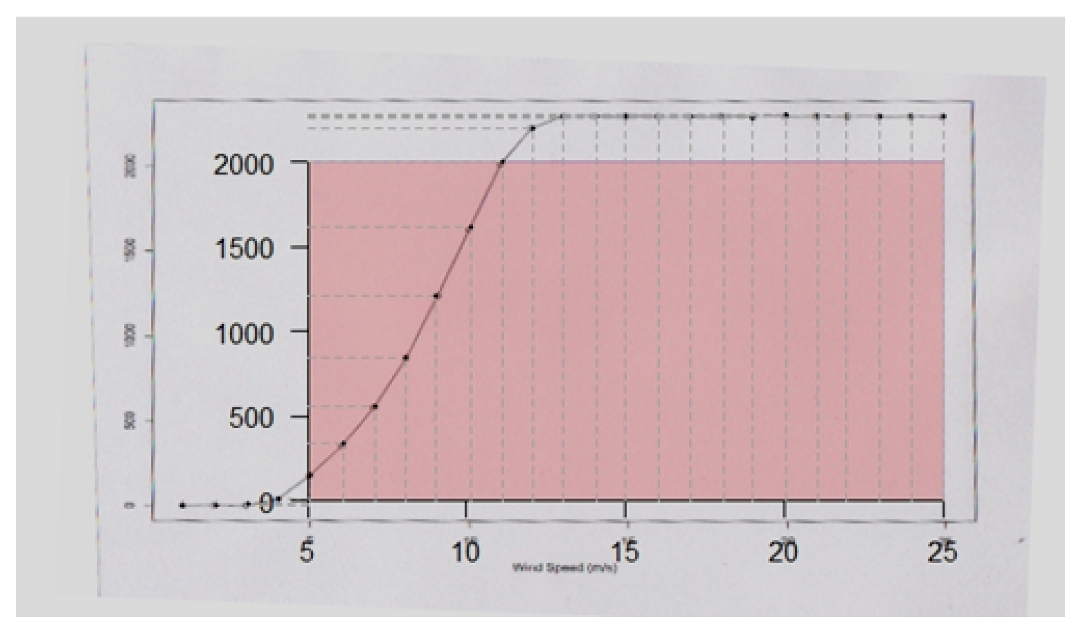
This example demonstrates how ‘WindCurves’ can be used as a useful tool for analyzing and fitting the WT power curves. The objective of this demonstration is to become aware of the procedures to be followed when using the ‘WindCurves’ package to fit the WT power curves. In an earlier section, the ‘Nordex N90’ dataset was fitted, whereas in this section, the discrete values of the power curve were extracted from the curve image shown in Figure A1.
Figure A1.
The WT power curve image to be supplied to ‘img2points()’ function.

Appendix A.3.1. Step 1: Extract Discrete Values of the Power Curve
This step involves two actions:
- 1.
- Select two extreme points on each X- and Y-axes (Figure A2).
In this state, the inclination angle of the image (if there is one) is informed to the user who is asked to decide whether to re-map the X- and Y-axes’ points in the image. Furthermore, it transforms the inclined image with a new and non-inclined image. If the user permits character “Y”, the ‘img2points()’ function will ask again to map the axes’ points, and a more accurate mapping is achieved. Otherwise, the following action is activated.
Figure A2.
Selection and mapping of two points on each X- and Y-axes.

- 2.
- Point to ‘n’ numbers of points on the power curve image. (Figure A3).
a <- img2points(“scanned_image.jpeg”, n = 25)
#> Click on leftmost point on X axis and then enter the value of the point:
#> Enter the value: 5
#> Click on rightmost point on X axis and then enter the value of the point:
#> Enter the value: 25
#> Click on lowermost point on Y axis and then enter the value of the point:
#> Enter the value: 0
#> Click on uppermost point on Y axis and then enter the value of the point:
#> Enter the value: 2000
#>
#> The image was tilted by -2.11550492800417 Degrees.
#> Do you wish to resize the Scale?(Y/N)
#> N
#>
#> Select desired 25 points on the curve:
#>
a
#> Speed Power
#> 1 1.033058 0.00000
#> 2 2.079890 0.00000
#> 3 3.016529 29.62963
#> 4 4.118457 44.44444
#> 5 5.000000 177.77778
#> 6 5.936639 370.37037
#> 7 6.983471 562.96296
#> 8 8.030303 874.07407
#> 9 9.022039 1244.44444
#> 10 10.068871 1644.44444
#> 11 11.060606 2014.81481
#> 12 11.997245 2222.22222
#> 13 12.988981 2311.11111
#> 14 14.035813 2311.11111
#> 15 15.027548 2311.11111
#> 16 16.019284 2311.11111
#> 17 17.011019 2311.11111
#> 18 18.002755 2311.11111
#> 19 18.994490 2325.92593
#> 20 20.041322 2311.11111
#> 21 20.977961 2325.92593
#> 22 22.024793 2325.92593
#> 23 23.016529 2325.92593
#> 24 24.008264 2325.92593
#> 25 25.000000 2325.92593
Figure A3.
Extraction of discrete points from the WT power curve.

Appendix A.3.2. Step 2: Fit the Curve for Discrete Values Extracted in Step 1 with the ‘fitcurve()’ Function
The default syntax for the ‘fitcurve()’ function is as follows.
b <- fitcurve(data = a)
In this example, the following sample curve fitting method ‘random()’ is added in the study.
random <- function(x)
{
data_y <- sort(sample(1:1500, size = 25, replace = TRUE))
d <- data.frame(data_y)
return(d)
}
b <- fitcurve(data = a,
MethodPath = "source(’~/curves/random.R’)",
MethodName = "Random Method")
#> Weibull CDF model
#> -----------------
#> P = 1 - exp[-(S/C)^k]
#> where P -> Power and S -> Speed
#>
#> Shape (k) = 4.292249
#> Scale (C) = 9.713117
#> ===================================
#>
#> Logistic Function model
#> -----------------------
#> P = phi1/(1+exp((phi2-S)/phi3))
#> where P -> Power and S -> Speed
#>
#> phi 1 = 2325.242
#> phi 2 = 8.690274
#> phi 3 = 1.39292
#> ===================================
b
#> $Speed
#> [1] 0.9668508 2.0718232 3.0662983 4.0607735 5.0552486 6.0497238 6.9889503
#> [8] 8.0386740 8.9779006 10.1381215 11.0220994 12.0165746 13.0662983 14.0607735
#> [15] 15.0000000 16.1049724 17.0441989 18.0386740 19.0331492 20.1381215 21.0220994
#> [22] 22.0165746 23.0110497 24.0607735 25.0000000
#>
#> Power
#> [1] 0.00000 0.00000 0.00000 44.44444 177.77778 355.55556 577.77778
#> [8] 888.88889 1229.62963 1629.62963 2000.00000 2237.03704 2296.29630 2311.11111
#> [15] 2311.11111 2311.11111 2311.11111 2311.11111 2311.11111 2296.29630 2311.11111
#> [22] 2311.11111 2311.11111 2296.29630 2296.29630
#>
#> ‘Weibull CDF‘
#> [1] 0.00000 0.00000 0.00000 97.48009 177.77778 322.83674 534.25616
#> [8] 856.98139 1200.39308 1629.62963 1905.45360 2123.71918 2247.36848 2294.10923
#> [15] 2307.55658 2310.75608 2311.07933 2311.10965 2311.11107 2311.11111 2311.11111
#> [22] 2311.11111 2311.11111 2311.11111 2311.11111
#>
#> ‘Logistic Function‘
#> [1] 0.00000 0.00000 0.00000 80.85006 159.32640 303.66882 529.43169
#> [8] 895.54047 1282.23262 1717.75136 1958.12353 2129.70846 2228.92454 2277.05646
#> [15] 2300.43863 2313.95630 2319.47823 2322.41612 2323.85754 2324.61579 2324.91021
#> [22] 2325.07976 2325.16280 2325.20498 2325.22338
#>
#> ‘Random Method‘
#> [1] 52 73 84 176 212 230 306 323 345 357 481 723 753 813 862
#> [16] 954 963 1114 1159 1206 1302 1379 1379 1384 1483
#>
#> attr(,"row.names")
#> [1] 1 2 3 4 5 6 7 8 9 10 11 12 13 14 15 16 17 18 19 20 21 22 23 24 25
#> attr(,"class")
#> [1] "fitcurve"$
Appendix A.3.3. Step 3: Compare the Fitted Curves
The default syntax for the ‘validate.curve()’ function is as follows.
validate.curve(x = b)
In this example, the following addition sample error metric ‘error()’ (which returns the RSME values) is added in the study, and corresponding fitted curves can be plotted as shown in Figure A4.
library(imputeTestbench)
error <- function(a,b)
{
c <- rmse(a,b)
return(c)
}
validate.curve(x = b,
MethodPath = "source(’~/curves/error.R’)", MethodName = "New Error")
#> Metrics Weibull CDF Logistic Function Random Method
#> 1 RMSE 36.2129522 39.8916751 1020.3785758
#> 2 MAE 20.5040548 29.0803404 870.4992593
#> 3 MAPE 4.2798325 5.0902950 132.7159241
#> 4 R2 0.9985355 0.9982228 -0.1627775
#> 5 COR 0.9993632 0.9991146 0.8734492
#> 6 New Error 36.2129522 39.8916751 1020.3785758
plot(b)
Figure A4.
The plot of the WT power curve fitted with the ‘fitcurve()’ function.

Appendix A.4. Discussion
The R package ‘WindCurves’ aims to enhance and speed up the research activities in the field of wind energy. The proposed package is quick and requires very little effort while working on WT power curves. This preliminary form of the package has included the Weibull CDF and logistic function methods, showing very promising results. Furthermore, it provides the provision to compare user-defined methods. The authors are looking positively towards encouraging researchers to contribute to this package for the betterment of our ecology systems.
References
- Nunnari, S.; Fortuna, L.; Gallo, A. Wind time series modeling for power turbine forecasting. Int. J. Electr. Energy 2014, 2, 112–118. [Google Scholar] [CrossRef]
- Fortuna, L.; Nunnari, G.; Nunnari, S. A new fine-grained classification strategy for solar daily radiation patterns. Pattern Recognit. Lett. 2016, 81, 110–117. [Google Scholar] [CrossRef]
- Bandi, M.M.; Apt, J. Variability of the wind turbine power curve. Appl. Sci. 2016, 6, 262. [Google Scholar] [CrossRef]
- Shokrzadeh, S.; Jozani, M.J.; Bibeau, E. Wind turbine power curve modeling using advanced parametric and nonparametric methods. IEEE Trans. Sustain. Energy 2014, 5, 1262–1269. [Google Scholar] [CrossRef]
- Ouyang, T.; Kusiak, A.; He, Y. Modeling wind-turbine power curve: A data partitioning and mining approach. Renew. Energy 2017, 102, 1–8. [Google Scholar] [CrossRef]
- Lydia, M.; Kumar, S.S.; Selvakumar, A.I.; Kumar, G.E.P. A comprehensive review on wind turbine power curve modeling techniques. Renew. Sustain. Energy Rev. 2014, 30, 452–460. [Google Scholar] [CrossRef]
- Villanueva, D.; Feijóo, A.E. Reformulation of parameters of the logistic function applied to power curves of wind turbines. Electr. Power Syst. Res. 2016, 137, 51–58. [Google Scholar] [CrossRef]
- Sohoni, V.; Gupta, S.; Nema, R. A critical review on wind turbine power curve modeling techniques and their applications in wind based energy systems. J. Energy 2016, 2016, 8519785. [Google Scholar] [CrossRef]
- Usaola, J. Probabilistic load flow in systems with wind generation. IET Gener. Trans. Distrib. 2009, 3, 1031–1041. [Google Scholar] [CrossRef] [Green Version]
- Aien, M.; Ramezani, R.; Ghavami, S.M. Probabilistic load flow considering wind generation uncertainty. Eng. Technol. Appl. Sci. Res. 2011, 1, 126–132. [Google Scholar]
- Harris, R.I. A simulation method for macro-meteorological wind speeds with a Forward Weibull parent distribution of general index. J. Wind Eng. Ind. Aerodyn. 2017, 171, 202–206. [Google Scholar] [CrossRef]
- Kaplan, O.; Temiz, M. A novel method based on Weibull distribution for short-term wind speed prediction. Int. J. Hydrog. Energy 2017, 42, 17793–17800. [Google Scholar] [CrossRef]
- Shi, L.B.; Weng, Z.X.; Yao, L.Z.; Ni, Y.X. An analytical solution for wind farm power output. IEEE Trans. Power Syst. 2014, 29, 3122–3123. [Google Scholar] [CrossRef]
- Tian, J.; Zhou, D.; Su, C.; Blaabjerg, F.; Chen, Z. Optimal control to increase energy production of wind farm considering wake effect and lifetime estimation. Appl. Sci. 2017, 7, 65. [Google Scholar] [CrossRef]
- Carrillo, C.; Cidrás, J.; Díaz-Dorado, E.; Obando-Montaño, A.F. An approach to determine the Weibull parameters for wind energy analysis: The case of Galicia (Spain). Energies 2014, 7, 2676–2700. [Google Scholar] [CrossRef]
- Scholz, F.W. Characterization of the Weibull distribution. Comput. Stat. Data Anal. 1990, 10, 289–292. [Google Scholar] [CrossRef]
- Freris, L.L. Wind Energy Conversion Systems; Prentice Hall: Upper Saddle River, NJ, USA, 1990. [Google Scholar]
- Jensen, N.O. A Note on Wind Generator Interaction; Risø: Roskilde, Denmark, 1983. [Google Scholar]
- Katic, I.; Højstrup, J.; Jensen, N.O. A simple model for cluster efficiency. In Proceedings of the European Wind Energy Association Conference and Exhibition, Rome, Italy, 7–9 October 1986. [Google Scholar]
- Feijóo, A.; Villanueva, D. Wind farm power distribution function considering wake effects. IEEE Trans. Power Syst. 2017, 32, 3313–3314. [Google Scholar] [CrossRef]
- Staffell, I. Wind Turbine Power Curves; Imperial College London: London, UK, 2012. [Google Scholar]
- Nwobi, F.N.; Ugomma, C.A. A comparison of methods for the estimation of Weibull distribution parameters. Metodol. Zvezki 2014, 11, 65. [Google Scholar]
- Al-Fawzan, M.A. Methods for Estimating the Parameters of the Weibull Distribution; King Abdulaziz City for Science and Technology: Riyadh, Saudi Arabia, 2000. [Google Scholar]
- Ahmed, S.A. Comparative study of four methods for estimating Weibull parameters for Halabja, Iraq. Int. J. Phys. Sci. 2013, 8, 186–192. [Google Scholar]
- Bokde, N.; Feijóo, A.E. WindCurves: Tool to Fit Wind Turbine Power Curves, R package version 0.1.2; The Comprehensive R Archive Network: Hoboken, NJ, USA, 2018. [Google Scholar]
- Beck, M.W.; Bokde, N.; Asencio-Cortés, G.; Kulat, K. R Package imputeTestbench to Compare Imputation Methods for Univariate Time Series. R J. 2018, 10, 218–233. [Google Scholar]
- Beck, M.W.; Bokde, N. ImputeTestBench: Test Bench for the Comparison of Imputation Methods, R package version 3.0.1; The Comprehensive R Archive Network: Hoboken, NJ, USA, 2017. [Google Scholar]
- Poisot, T. The digitize package: Extracting numerical data from scatterplots. R J. 2011, 3, 25–26. [Google Scholar]
- Bunn, A.; Korpela, M. R: A Language and Environment for Statistical Computing; R Foundation for Statistical Computing: Vienna, Austria, 2018. [Google Scholar]
- Jefferis, G. Readbitmap: Simple Unified Interface to Read Bitmap Images (BMP, JPEG, PNG), R package version 0.104; The Comprehensive R Archive Network: Hoboken, NJ, USA, 2014. [Google Scholar]
Figure 1.
Representation of Equation (5) in the form of a straight line.
Figure 1.
Representation of Equation (5) in the form of a straight line.

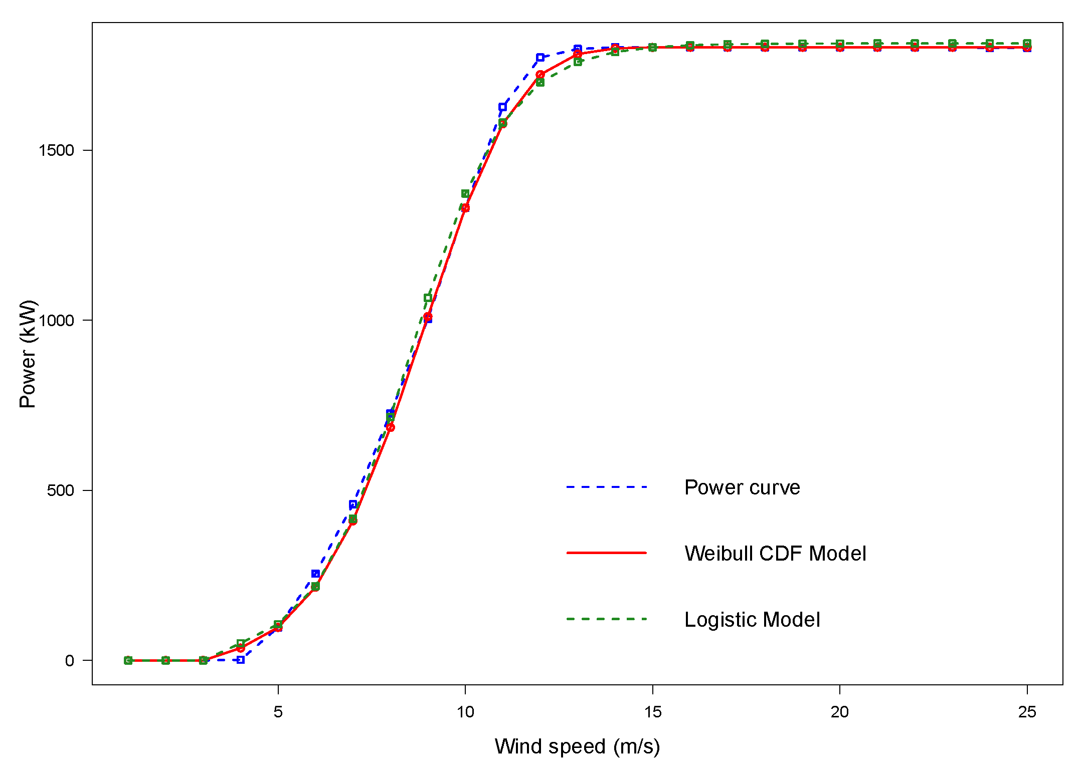
Figure 2.
Weibull CDF and 4P-OP models for the Vestas V80 2-MW power curve.

Figure 3.
Weibull CDF and 4P-OP models for the Siemens 82 2-MW power curve.

Figure 4.
Weibull CDF and 4P-OP models for the REpower 82 2050-kW power curve.

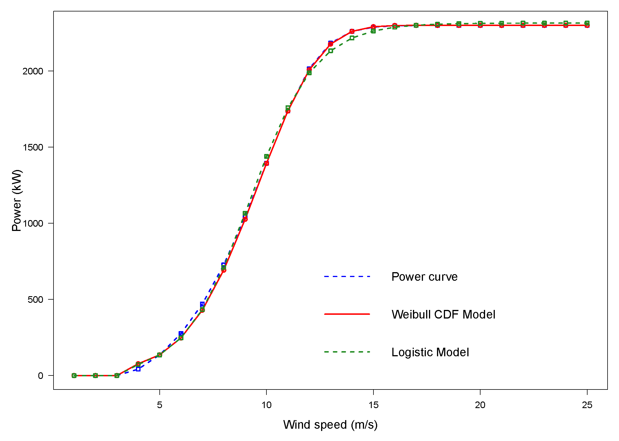
Figure 5.
Weibull CDF and 4P-OP models for the Nordex N90 2-MW power curve.

Figure 6.
Weibull CDF and 4P-OP models for the Siemens 107 2-MW power curve.

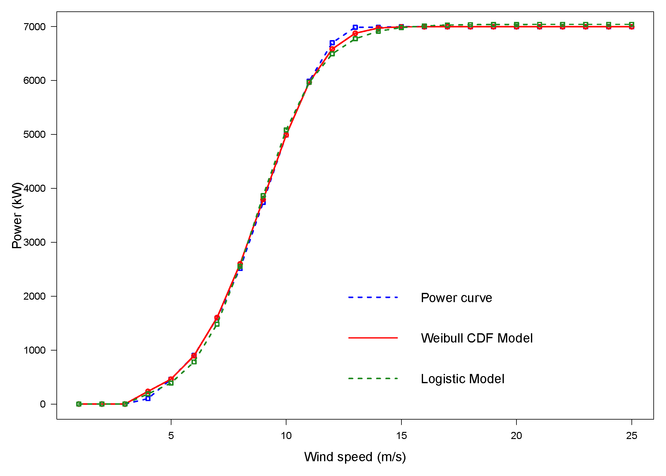
Figure 7.
Weibull CDF and 4P-OP models for the Vestas V164 2-MW power curve.


Table 1.
Symbols used in the following sections.
| Symbols | Meaning |
|---|---|
| CDF of wind speed series | |
| P | a function of wind speed |
| maximum WT power | |
| minimum WT power | |
| calculated power with proposed function | |
| specified power (values given by the manufacturers) | |
| k | shape parameter |
| C | scale parameter |
| v | hub height |
| the thrustcoefficient | |
| the Waledecay constant | |
| d | the distance between WTs |
| D | the rotor diameter of WTs |
| wake coefficient | |
| the mean value of coefficient of mWTs |
Table 2.
Values of parameters ‘k’ and ‘C’ for several WTs using the proposed model.
| Model | Vestas V80 | Siemens 82 | REpower 82 | Nordex N90 | Siemens 107 | Vestas V164 |
|---|---|---|---|---|---|---|
| k | 4.6256 | 4.4233 | 4.5242 | 4.2424 | 4.5699 | 4.5241 |
| C | 9.3890 | 10.2096 | 9.7374 | 9.5649 | 9.8116 | 9.5458 |
Table 3.
Comparison of RMSE values for several WTs.
| Model | Vestas V80 | Siemens 82 | REpower 82 | Nordex N90 | Siemens 107 | Vestas V164 |
|---|---|---|---|---|---|---|
| 4P-OP | 25.3319 | 24.5692 | 21.2895 | 39.1501 | 42.6797 | 96.6218 |
| 4P-DP | 56.2597 | 59.9937 | 38.1073 | 68.3914 | 85.3121 | 146.1193 |
| 4P-DS | 55.4600 | 54.6059 | 35.5069 | 65.3848 | 80.6301 | 129.8385 |
| Weibull CDF | 22.0624 | 14.5216 | 18.3741 | 30.8761 | 20.1724 | 46.5722 |
Table 4.
Comparison of MAE values for several WTs.
| Model | Vestas V80 | Siemens 82 | REpower 82 | Nordex N90 | Siemens 107 | Vestas V164 |
|---|---|---|---|---|---|---|
| 4P-OP | 19.2696 | 18.1581 | 16.0462 | 27.1972 | 31.4132 | 60.5502 |
| 4P-DP | 32.4614 | 34.7689 | 24.3311 | 38.8846 | 51.3634 | 89.9470 |
| 4P-DS | 36.9029 | 37.5170 | 23.2441 | 41.6216 | 53.3197 | 77.3338 |
| Weibull CDF | 11.7565 | 7.0023 | 9.4974 | 15.1381 | 10.3209 | 22.1550 |
Table 5.
Best case values of parameters ‘k’ and ‘C’ for several WTs.
| Model | Vestas V80 | Siemens 82 | REpower 82 | Nordex N90 | Siemens 107 | Vestas V164 |
|---|---|---|---|---|---|---|
| k | 4.57 | 4.13 | 4.08 | 4.36 | 4.54 | 4.53 |
| C | 9.29 | 10.11 | 9.55 | 9.43 | 9.80 | 9.50 |
Table 6.
Comparison of the RMSE and MAE values for the best case parameters.
| Model | Vestas V80 | Siemens 82 | REpower 82 | Nordex N90 | Siemens 107 | Vestas V164 |
|---|---|---|---|---|---|---|
| RMSE | 18.1487 | 10.8834 | 11.2334 | 25.9851 | 19.8567 | 43.2761 |
| MAE | 10.66565 | 6.9250 | 6.8415 | 14.06718 | 9.2265 | 21.4085 |
© 2018 by the authors. Licensee MDPI, Basel, Switzerland. This article is an open access article distributed under the terms and conditions of the Creative Commons Attribution (CC BY) license (http://creativecommons.org/licenses/by/4.0/).
Share and Cite
MDPI and ACS Style
Bokde, N.; Feijóo, A.; Villanueva, D. Wind Turbine Power Curves Based on the Weibull Cumulative Distribution Function. Appl. Sci. 2018, 8, 1757. https://doi.org/10.3390/app8101757
AMA Style
Bokde N, Feijóo A, Villanueva D. Wind Turbine Power Curves Based on the Weibull Cumulative Distribution Function. Applied Sciences. 2018; 8(10):1757. https://doi.org/10.3390/app8101757
Chicago/Turabian StyleBokde, Neeraj, Andrés Feijóo, and Daniel Villanueva. 2018. "Wind Turbine Power Curves Based on the Weibull Cumulative Distribution Function" Applied Sciences 8, no. 10: 1757. https://doi.org/10.3390/app8101757
Note that from the first issue of 2016, this journal uses article numbers instead of page numbers. See further details here.