Collision Avoidance from Multiple Passive Agents with Partially Predictable Behavior

Abstract

Navigating a robot in a dynamic environment is a challenging task, especially when the behavior of other agents such as pedestrians, is only partially predictable. Also, the kinodynamic constraints on robot motion add an extra challenge. This paper proposes a novel navigational strategy for collision avoidance of a kinodynamically constrained robot from multiple moving passive agents with partially predictable behavior. Specifically, this paper presents a new approach to identify the set of control inputs to the robot, named control obstacle, which leads it towards a collision with a passive agent moving along an arbitrary path. The proposed method is developed by generalizing the concept of nonlinear velocity obstacle (NLVO), which is used to avoid collision with a passive agent, and takes into account the kinodynamic constraints on robot motion. Further, it formulates the navigational problem as an optimization problem, which allows the robot to make a safe decision in the presence of various sources of unmodelled uncertainties. Finally, the performance of the algorithm is evaluated for different parameters and is compared to existing velocity obstacle-based approaches. The simulated experiments show the excellent performance of the proposed approach in term of computation time and success rate.

1. Introduction

Motion planning in dynamic environments has become central to the operations of robots. Most modern applications require navigation of robots among humans, vehicles and other robots. Almost all of the mobile robots in the real world applications are subjected to kinodynamic constraints like differential driven or car-like robots [1,2]. Many different kinds of motion planning algorithms have been developed for such robots facing static environment, and then they were further extended for dynamic environments. In [3], a motion planning approach for the car-like robots was presented, and it was proved that the path for holonomic robots lying in an open configuration space could be transformed into an equally useful path for nonholonomic robots. Particularly, an algorithm was proposed to generate a useful path for nonholonomic systems based on the path obtained for holonomic robots. However, that transformation was not smooth for car-like robots. It was first proposed in [4] and their idea was further improved in [5]. However, instead of using a steering function, authors presented a method based on computing clothoid curves. Although their method improved transition and smoothness, authors did not address complete trajectory planning for dynamic environments. For this propose many authors have proposed different algorithms focusing on complete trajectory planning , such as [6,7,8]. In some of these works, the problem of robot motion planning in a dynamic environment was decomposed into hatching an achievable path for nonholonomic systems, and designing a velocity profile by which such vehicles could maneuver safely [9,10,11]. However, these approaches do not perform well for navigating a robot in a dynamic environment with multiple moving agents, like pedestrian environment, due to following reasons. (1) These approaches do not take into account the future prediction of obstacle motion thus robot being blinded to a potential collision. (2) When planning in such dynamic environment the time available to compute solution is limited, it is the function of nature and dynamicity of the environment. Therefore, in a highly dynamic environment there is a high probability that a complete path to the goal cannot be computed in the available time.

In [12,13], the problem of kinodynamic motion planning for a robot in a dynamic environment was addressed. The proposed approaches explore the state-time space of the robot to find a collision free path to the goal, while it was assumed that the entire path of the passive agents is known. However, this assumption restricts their application when extending them to pedestrian or multi-agent environment. In most of the applications of navigating an agent, the moving obstacles has free will, and their future behavior is only partially predictable (if at all). When facing such situation, obstacle’s path must be predicted using prediction techniques such as the ones presented in [14,15,16,17]. When the on-line path prediction is used to plan motion, it is likely that the model of the future that is obtained will have limited time duration. In addition, such on-line prediction is noisy. Therefore, a planner is required that takes into account the validity duration of the model of the environment and allowable time for computing a solution. Also, it is necessary to consider various sources of uncertainties present, e.g., passive agents unpredictability, uncertainty in resulting state under a given control action, and localization error.

Some of the principal work that considers the future behavior of pedestrians or other kind of agents is focused on the concept of velocity obstacle (VO) [18]. The original formulation of VO was designed for an agent with simple-agent dynamics to avoid a collision with a passive agent moving along a known straight path. In [19], authors proposed an optimal reciprocal collision avoidance strategy (ORCA) for multiple active agents, considering similar behavior for all agents. More specifically, the work assumes that each agent employs a similar collision avoidance strategy. Instead of complete motion planning, their approach was to plan local motion directed towards the next (sub) goal extracted from a global way point plan. Several efforts have been made to extend the concept of ORCA to more complex dynamic systems ranging from the single integrator, differential driven, car-like robot and arbitrary linear equation of motion in [20,21,22,23,24,25]. However, these approaches require every agent in a collision to run a similar collision avoidance algorithm. In [26], authors examined the issue of navigating car-like agent in the dynamic environment with multiple passive agents. They extended the concept of VO to consider the constraint of the kinematic car-like agent to avoid collision with passive agents moving along the linear path. The approach was designed for specific agent dynamics and cannot be simply extended for avoiding passive agents moving along an arbitrary path, probably nonlinear.

1.1. Contribution

This paper addresses the problem of navigating a kinodynamically constrainted robot, among multiple passive agents with partially predictable behavior. In order to solve the problem, this paper develops the following two contributions.

• First, it generalizes the concept of Nonlinear velocity obstacle (NLVO) [27] to develop a new approach to identify the set of control inputs to robot that will lead the robot towards collision, named control obstacle. It seeks to address the issue of navigating a robot with kinodynamic constraints while considering that a passive agent is moving along an arbitrary path, probably non-linear. The original approach of NLVO does not consider the robot model, and thus is limited to the agent with dynamics as of single integrator.
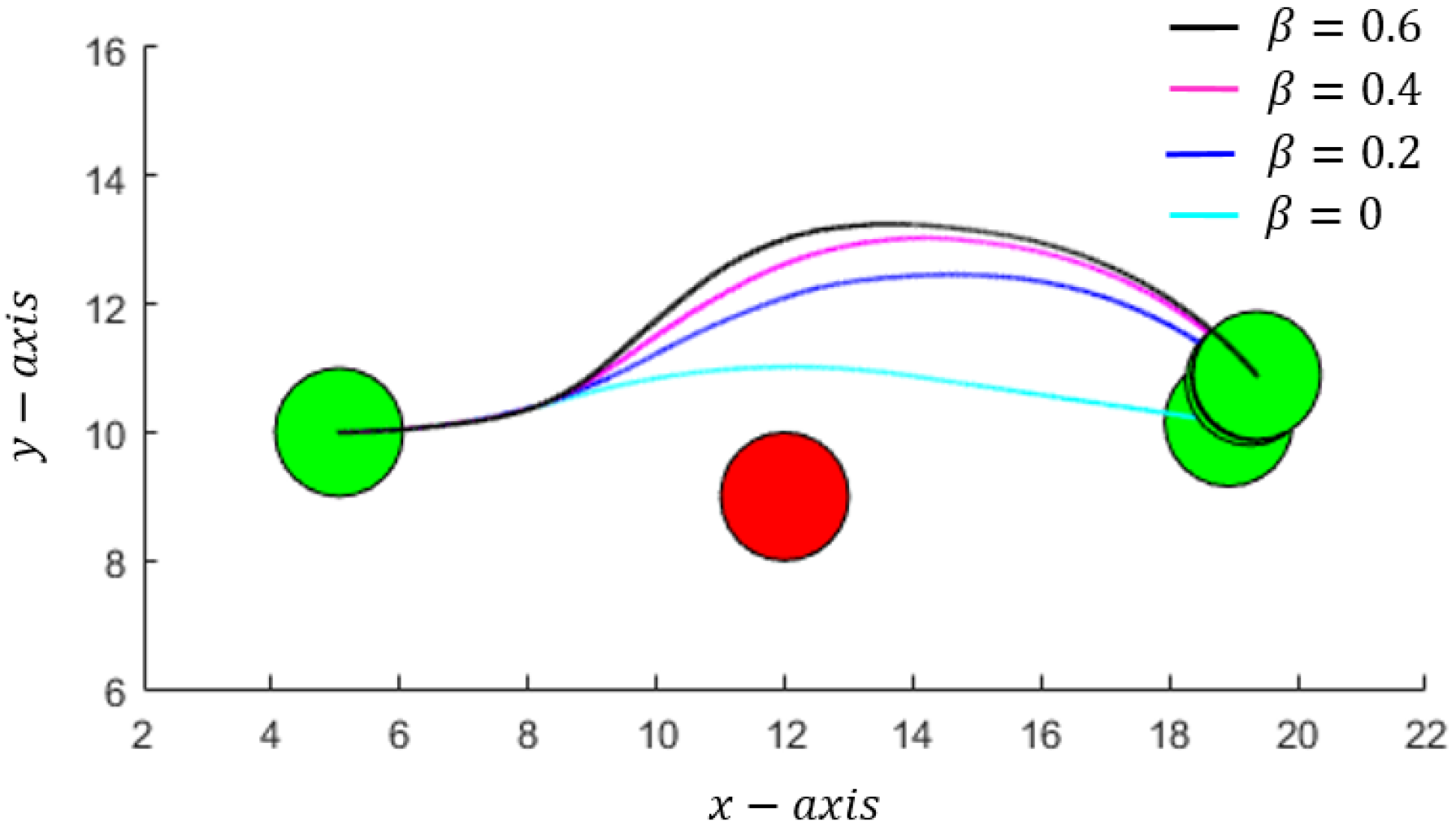
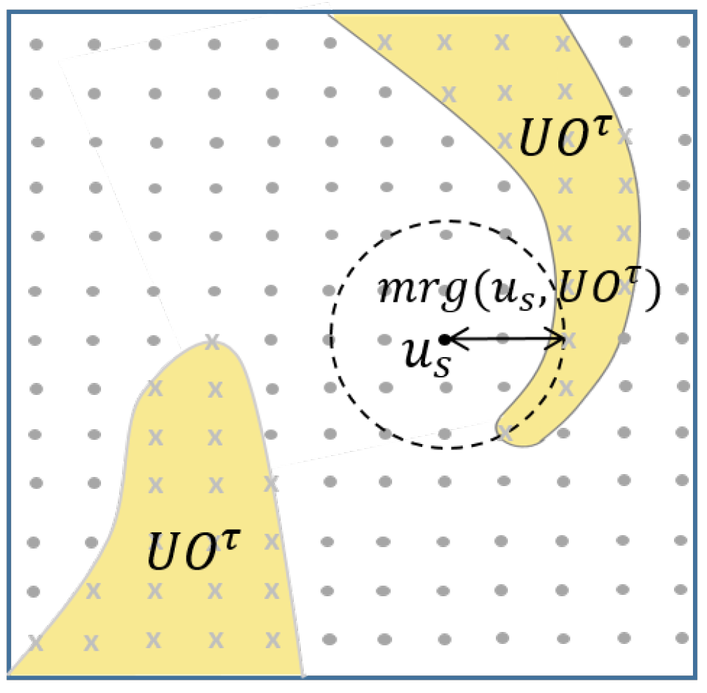
• Secondly, a novel collision avoidance strategy is proposed, that allows the robot to make a safe decision for avoiding a collision with the passive agents. The safe navigation decision is based on the concept of minimum safety margin which is the measure of how safe the path is in the presence of various sources of unmodeled uncertainties.

This paper presents the implementation of the proposed approach for a car-like agent and a double integrator. The performance of the proposed algorithm is evaluated for dynamic environment considered in [26], where the predicted trajectory of passive agents change frequently. The simulated experiments show better performance of the proposed approach compared to current VO based approaches, in terms of computation time and success rate.

1.2. Limitations

As this work extends the concept of velocity obstacle that increases its applicability, it inherits some limitations of VO method. First, it requires the passive agents to be of circular shape. It is a logical assumption for pedestrians or mobile robots, as it simplifies the problem. For a non-circular passive agent, collision avoidance is achieved by selecting a circle enclosing geometry of a passive agent. Second, this work proposes a local navigation approach. Thus it requires a global motion planner to converge to goal in the presence of the large static obstacles. The paper presents one possible implementation of the global navigational plan in Section 5, which results in model predictive partial motion planning framework.

Finally, the presented approach is probabilistic in nature. It is possible that in some cases the solution may not be found even if one exists. However, simulation results show that the presented approach has much higher success rate compared to existing VO based approaches.

1.3. Organization

The rest of this paper is organized as follows. Section 2 discusses the previous work done relating to VO based navigation. Section 3 reviews the nonlinear velocity obstacle and the issue that appears when applying it to navigate a kinodynamically constrained agent. Section 4 introduces the idea of a control obstacle and describes the safe margin input space. Section 5 presents the proposed navigation approach. Section 6 presents the implementation of the proposed approach for robot dynamics as of the double integrator and a car-like robot. Further, this section evaluates the performance of the algorithm for a set of parameters and compares the performance of the proposed approach with current approaches. Finally, Section 7 concludes the paper.

2. Previous Work

One of the early development in collision avoidance is of velocity obstacle (VO) [18]. VO is a cone in the velocity space of agent, which represents the set of velocities that will lead an active agent towards a collision with a passive agent. To avoid the collision, active agent has to select its velocity outside VO. The early approach was developed for simple agent dynamics to avoid collision with a passive agent which is moving along a straight path with constant velocity. In [27], authors proposed NLVO algorithm, which expands the concept of VO to allow an agent with linear equation of motion to avoid collision with a passive agent with known, possibly nonlinear trajectories. The generalized velocity obstacle (GVO) algorithm proposed in [26] does principally the opposite of NLVO. It considers a problem of car-like agent avoiding passive agents moving along linear paths.

In contrast of avoiding passive agents in [19], authors examined the issue of collision avoidance among active agents and proposed the concept of reciprocal collision avoidance. The approach was based on dividing the responsibility for collision avoidance among agents involved in a collision. Their approach generates collision free piecewise paths for active agents. Efforts have been made to extend the applicability of this approach to consider the kinodynamic constraints of agents. In [23], authors proposed the concept of Acceleration-Velocity Obstacle, (AVO), that takes into account the acceleration constraints of the robot. In [24], authors proposed the idea of continuous control obstacle, to generate a continuous collision free path rather than piecewise linear path. All these reciprocal collision based approaches require that all dynamic objects should employ the same algorithm to avoid a collision. Thus, these approaches cannot easily be extended for avoiding a collision with passive agents moving along an arbitrary path, possibly nonlinear and only partially predictable.

3. Background

This section will review the concept of nonlinear velocity obstacle proposed in [27] and discuss its application for a robot with kinodynamic constraints.

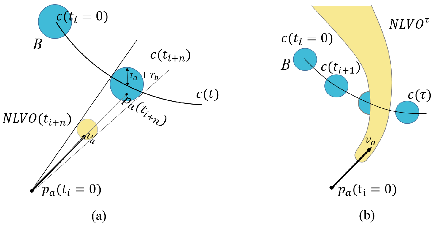
3.1. Nonlinear Velocity Obstacle

For a disc-shaped robot $R_a$ and moving obstacle $O_b$ of radii $r_a$ and $r_b$, respectively, the nonlinear velocity obstacle (NLVO) induced for $R_a$ is a set of its velocities that will result in its collision with $O_b$ at some time in the future. NLVO is defined in terms of its temporary components. Let at current time $t=0$, the center of the robot represented by $p_a\left(0\right)$ is at origin. In a robot configuration space, let set B represent the obstacle’s circular geometry with radius equal to the sum of radii $r_a$ and $r_b$, and the robot geometry is represented by a point, as shown in Figure 1a. For an obstacle following a generalized trajectory $c\left(t\right)$, the temporary velocity obstacle induced for a robot due to obstacle’s position at time instant $t_{i+n}$ is as follows:

$$\begin{array}{c}\hfill NLVO\left(t_{i+n}\right)=\frac{c\left(t_{i+n}\right)\oplus B}{t_{i+n}}\end{array}$$

(1)

where $c\left(t_{i+n}\right)\oplus B$ denotes the Minkowski sum of vector $c\left(t_{i+n}\right)$ and set B. $NLVO\left(t_{i+n}\right)$ is a set of all absolute velocities of a robot that will result in a collision of $p_a$ with a point in B at time instant $t_{i+n}$. The set of robot velocities that will result in collision of $p_a$ with B within time horizon $[0,\tau ]$ can be defined in terms of $NLVO\left(t_{i+n}\right)$ as follows:

$$\begin{array}{c}\hfill NLV{O}^{\tau }=\bigcup _{0<t\le \tau }NLVO\left(t\right)\end{array}$$

(2)

Geometrically, $NLV{O}^{\tau }$ is a warped cone, such as the one shown in Figure 1b.

Collision avoidance is then achieved as follow: Robot $R_a$ selects its new velocity at time $t=0$ such that $v_a\notin NLV{O}^{\tau }$ to remain safe for at least $\tau$ seconds into the future. The new velocity is usually selected that minimize the Euclidean distance to velocity $v_{pref}$, which in turn points to next sub goal extracted from global waypoint plan. $v_a$ is then applied for short time horizon until a next control loop begins.

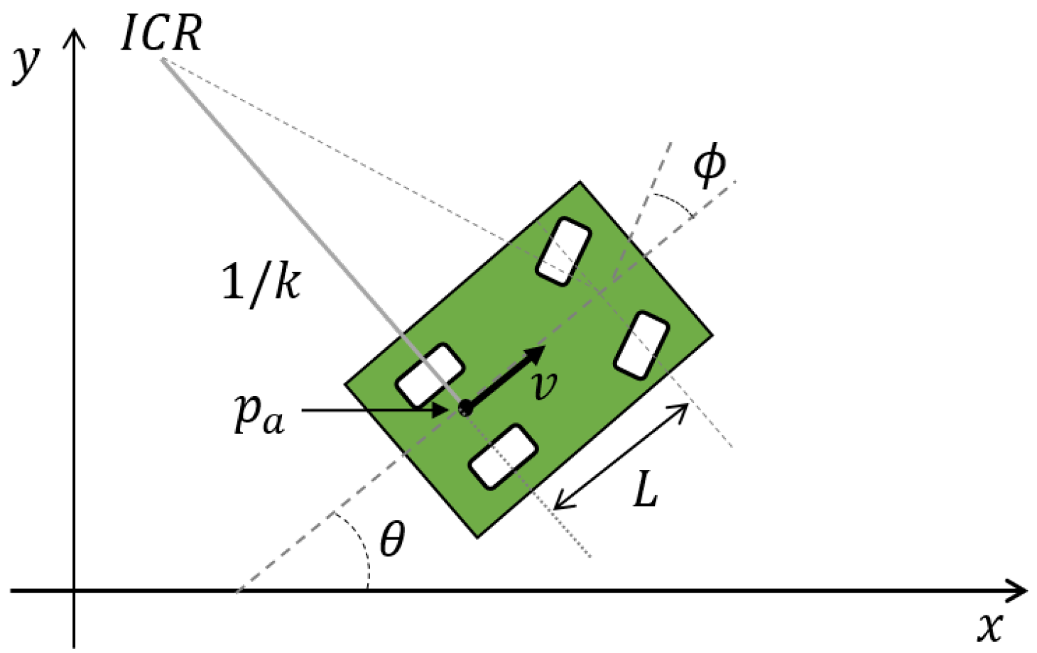
3.2. Robot with Kinodynamic Constraints

For a known, possibly nonlinear trajectory of a passive agent, NLVO defines the set of velocities that may lead the robot towards a collision with a passive agent into the future. For an arbitrary starting point, a new velocity outside $NLV{O}^{\tau }$ cannot be attained instantly by a mobile robot under kinodynamic constraints. For example, the robot with car-like dynamics, as shown in Figure 2, has feasible velocity in a single direction, specifically in the direction of rear wheels. If the current velocity of robot is in $NLV{O}^{\tau }$, a new velocity outside $NLV{O}^{\tau }$ can only be attained over some finite time, and there is no guarantee that a robot can attain that new velocity into the future without having a collision.

4. Safe Margin Control Space

This section presents a new concept of temporary control obstacle. It is the generalization of temporary velocity obstacle. It seeks to address the problem of computing collision free motion by taking the kinodynamic constraints of the robot into account. Secondly, it introduces the idea of safe margined control space to select the safest trajectory in the presence of various sources of uncertainties.

4.1. Passive Agent Representation

This work assumes that there is a system other than a robot, like the one presented in [16,17], that tracks passive agents, predicts their future behaviors, and presents them in a general format, used in this paper. We are given a list of the passive agents and each passive agent is considered to be a disc or sphere having a radius and a trajectory. The future behavior of a passive agent is represented in the form of set points that represent predicted future states of the passive agent, specifying its position and time.

4.2. Notations and Assumptions

Let the state space of robot A be $X_a$$\subset {\mathbb{R}}^{\mathbb{N}}$. The dimension of robot workspace is typically either $d=2$ or $d=3$. It is assumed that the position of the robot $p_a$ in configuration space can be obtained from its states $x_a\left(t\right)$, potentially by some nonlinear projection function $f:X_a⟶{\mathbb{R}}^d$.

$$\begin{array}{c}\hfill p_a\left(t\right)=f\left(x_a\left(t\right)\right)\end{array}$$

(3)

Let the control space of robot has the same dimension as the workspace. A constraint c defined on the robot states by constraint function $q_c(x_a\left(t\right),t)$ bounded in $\left[C_{-},C_{+}\right]$$(C_{-},C_{+}\in \mathbb{R})$ will constraint the allowable control inputs in the robot control space. It is assumed that this constrained control region is convex. In the case of multiple constraints defined on robot states an admissible control space represented by $U_{ad}$ is obtainable by taking the intersection of allowable control regions induced by each constraint.

Lets the continuous time state transition is given by some potential nonlinear function g: $X_a\times U_{ad}⟶{\mathbb{R}}^{\mathbb{N}}$

$$\begin{array}{c}\hfill {\dot{x}}_a\left(t\right)=g(x_a\left(t\right),u\left(t\right))\end{array}$$

(4)

where $x_a\left(t\right)$ is the state of the robot and $u\left(t\right)$ is the control input given to it. For the current state $x_a\left(t\right)=x_a\left(0\right)$ and constant control $u\left(t\right)=u\left(0\right)$, the state of the robot at $t>0$ is given by:

$$\begin{array}{c}\hfill x_a\left(t\right)=h(x_a,u,t)\end{array}$$

(5)

where $h:X_a\times U_{ad}\times \mathbb{R}⟶X_a$ is the solution of (4) which is considered to be obtainable by its integration.

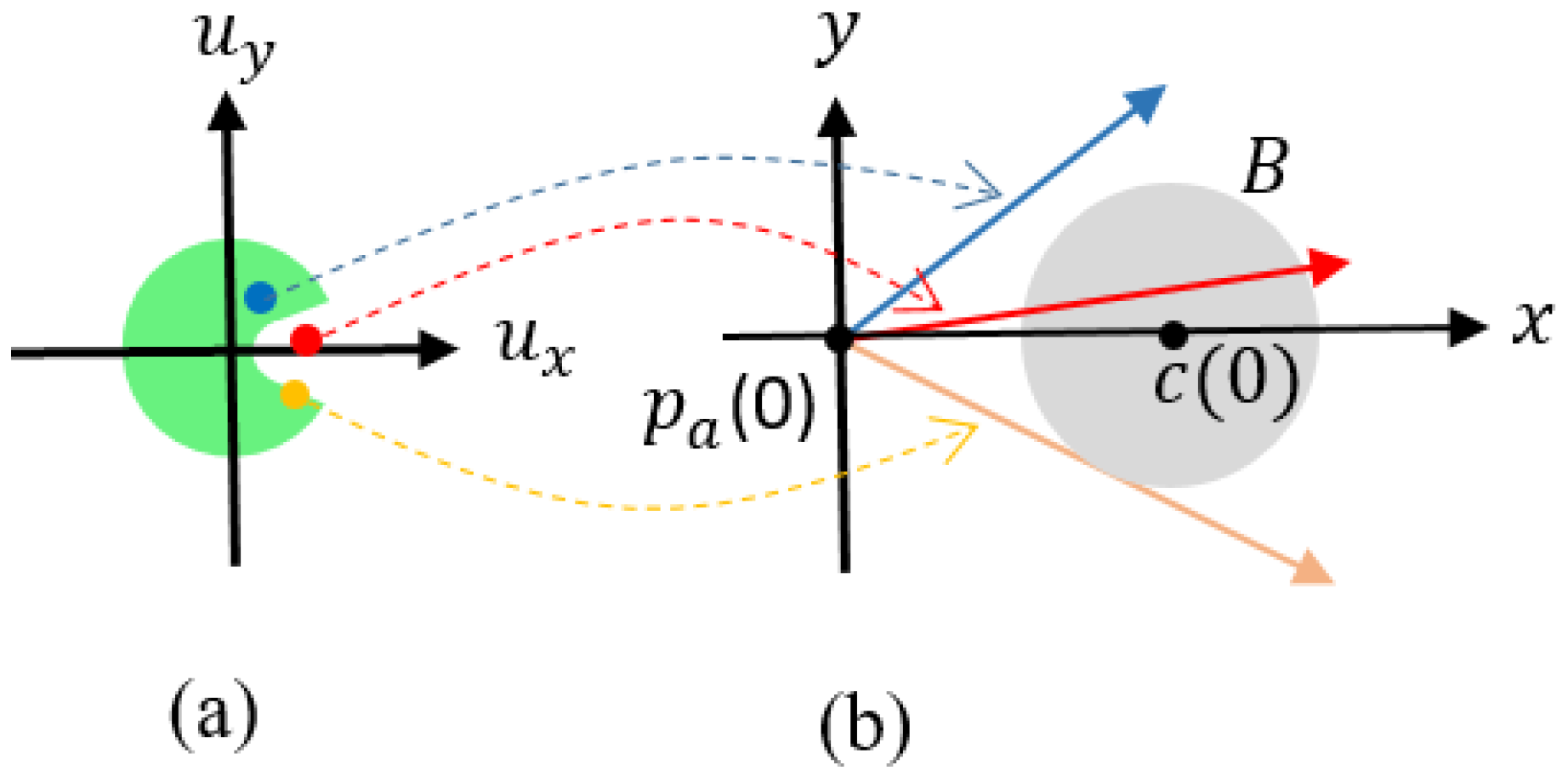
4.3. Control Obstacle

Consider a mobile robot that shares its workspace with multiple other passive agents. Let A and $B_j$ are the geometry of the robot and the $jth$ passive agent respectively. The robot and passive agent geometries are considered as their bounding circles, similarly as in the original formulation of $VO$ [18]. Let $O_j$ is the Minkowski sum of robot’s and $jth$ passive agent’s geometries, $O_j=A\oplus B_j$. The current position of passive agent is $c_j\left(0\right)$ and its position at $t>0$ is given by $c_j\left(t\right)$. To avoid collision with a passive agent within time horizon $\tau$, their relative position should remain outside the Minkowski sum of their geometries.

$$\begin{array}{c}\hfill p_a\left(t\right)-c_j\left(t\right)\notin O_j,\forall t\in [0,\tau ]\end{array}$$

(6)

Therefore, the temporary control obstacle induced due to the state of the $jth$ passive agent at a future time instant $t_{i+n}\in [0,\tau ]$, denoted by $U{O}_j\left(t_{i+n}\right)$, is defined as follows:

Definition 1.

(Temporary Control Obstacle) It is a set of control inputs for which the relative position vector is inside $O_j$ at time $t_{i+n}$

$$\begin{array}{c}\hfill U{O}_j\left(t_{i+n}\right)=\left\{u\right|f\left(h(x_a,u,t_{i+n})\right)-c_j\left(t_{i+n}\right)\in O_j\}\end{array}$$

(7)

where $f\left(h(x_a,u,t_{i+n})\right)-c_j\left(t_{i+n}\right)$ is a relative position vector at time $t_{i+n}$, for control input u given to a robot.

Now, the control obstacle induced for a robot due to the predicted motion of jth passive agent over the time horizon $[0,\tau ]$ can be defined as follows:

Definition 2.

(Control Obstacle) The control obstacle induced due to the states of a passive agent over time horizon $[0,\tau ]$ is the union of temporary control obstacles over that horizon.

$$\begin{array}{c}\hfill U{O}_j^{\tau }=\bigcup _{0<t_{i+n}\le \tau }U{O}_j\left(t_{i+n}\right)\end{array}$$

(8)

$U{O}_j^{\tau }$ is the set of control inputs to a robot, that will lead it towards collision with a passive agent in time horizon $[0,\tau ]$ into the future. In another words, the collision will not occur between the robot and passive agent $B_j$ with in time horizon $[0,\tau ]$ into the future, if robot selects its control input such that $u\notin U{O}_j^{\tau }$.

In case of avoiding collision from multiple passive agents, we can extend the given approach as follows. Let $N=\{1,...,m\}$ is the index of passive agents to be avoided. Then the control obstacle can be given as:

$$\begin{array}{c}\hfill U{O}^{\tau }=\bigcup _{j\in N}U{O}_j^{\tau }\end{array}$$

(9)

Robot selecting its control input outside $U{O}^{\tau }$ will lead it to move without collision with m passive agents within time horizon $[0,\tau ]$ into the future.

4.4. Safe Control Inputs

All control inputs in admissible control space that are not in control obstacle are considered as safe control inputs. The definition of safe control space is as follows:

Definition 3.

(Safe control space) It is the relative complement of $U{O}^{\tau }$ in $U_{ad}$.

$$\begin{array}{c}\hfill U_{safe}^{\tau }=U_{ad}\backslash U{O}^{\tau }\end{array}$$

(10)

Although all control inputs in $U_{safe}^{\tau }$ are considered safe, but each control input has a different level of proximity to the control obstacle. One possible metric defining the closeness of a safe control input $u_s\in U_{safe}^{\tau }$ to a control obstacle is defined in below definition.

Definition 4.

(Margin) The margin of safe control input $u_s$ is its minimum weighted distance to the control obstacle.

$$\begin{array}{c}\hfill mrg(u_s,U{O}^{\tau })=\underset{u\in U{O}^{\tau }}{min}\sqrt{{(u-u_s)}^{T}M(u-u_s)}\end{array}$$

(11)

where M is a positive definite diagonal weighted matrix whose values are assigned based on the importance of $jth$ dimension of control space.

The maximum margined control input is considered to be the safest control input to a robot, considering the various sources of unmodeled uncertainties.

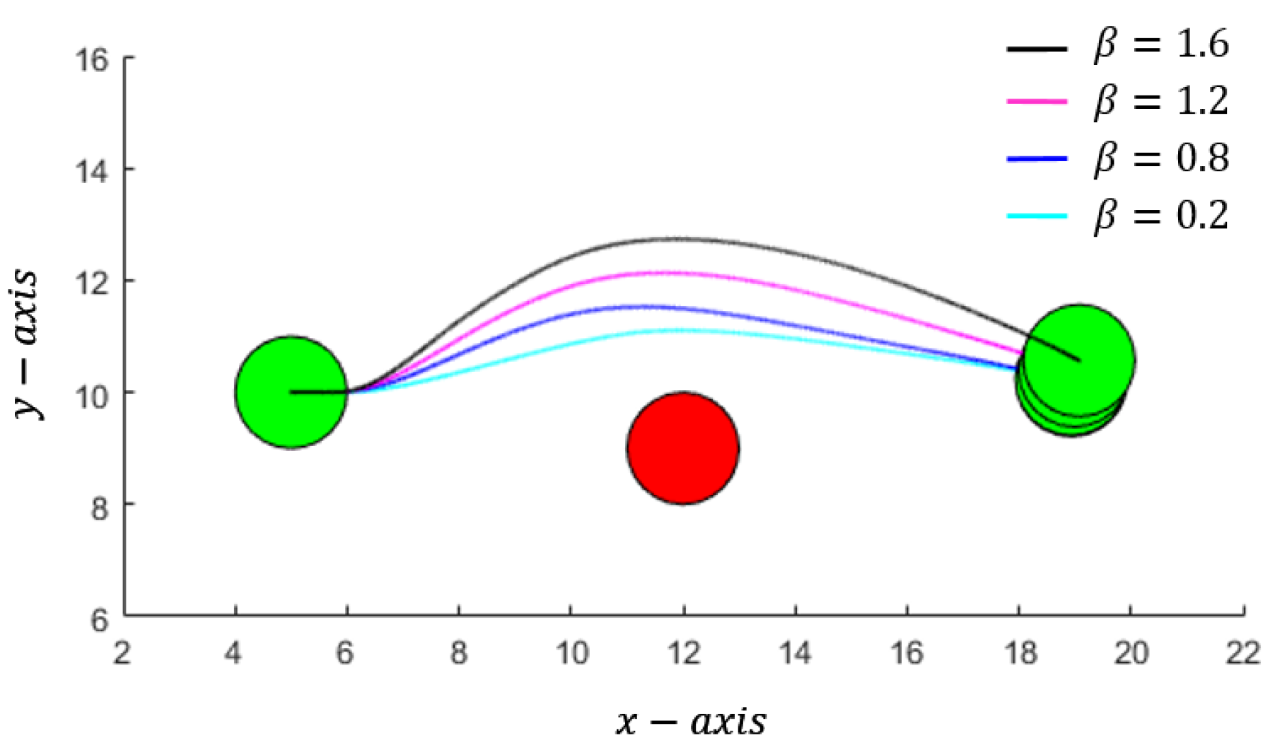
4.5. Example: Robot as Single-Integrator

To illustrate the concept of safe control space, take an example of a simple robot $R_A$ that was considered in [27]. The position of the center of a disc-shaped robot $R_A$, at time t, for a given control input u, is given as

$$\begin{array}{c}\hfill p_a(t,u)=p_a\left(0\right)+tu\end{array}$$

(12)

where $p_a\left(0\right)$ is the current position of robot. Similarly to [19], consider the constraint on robot states as follow:

$$\begin{array}{c}\hfill \sqrt{\dot{x}{\left(t\right)}^2+\dot{y}{\left(t\right)}^2}\in [0,v_m]\end{array}$$

(13)

where $v_m$ is the maximum speed of the robot. For system in (12), the control input directly corresponds to the velocity of the system ${\dot{p}}_a(t,u)=u$; therefore, $U_{ad}$ is a set of control inputs to a robot such that $\left|\right|u\left|\right|\le v_m$. Geometrically, $U_{ad}$ is a disc of the radius $v_m$ with its center at the origin in the control space.

The temporary control obstacle $U{O}_j\left(t_{i+n}\right)$ is the set of control inputs for which $p_a(t_{i+n},u)-c\left(t_{i+n}\right)\in B$. For the single integrator, temporary control obstacle is equivalent to temporary velocity obastcle, $NLVO\left(t_{i+n}\right)$ defined in [27], and is shown in Figure 1a. Geometrically, it is a disc of the radius $(r_a+r_a)/t_{i+n}$ with its center at $(c\left(t_{i+n}\right)-p_a\left(0\right))/t_{i+n}$ in robot control space .

Consider the following situation of the robot:

• current position at $p_a\left(0\right)=(0,0)$, radius $r_a=0.4$, and maximum linear speed limit of 1unit/s.
• disc shaped static obstacle of radius $r_b=0.4$ centered at $(2,0)$.
• temporary control obstacle considered at every time step of 0.1 s up to time horizon of $\tau =5$ s.

Figure 3 shows the obtained safe velocity space and the path undertaken by a robot for selected velocities with different margins.

5. Navigational Approach

This section will address the problem of navigating a robot among multiple passive agents. It further discusses a possible global navigation plan for navigating a robot among large static obstacles.

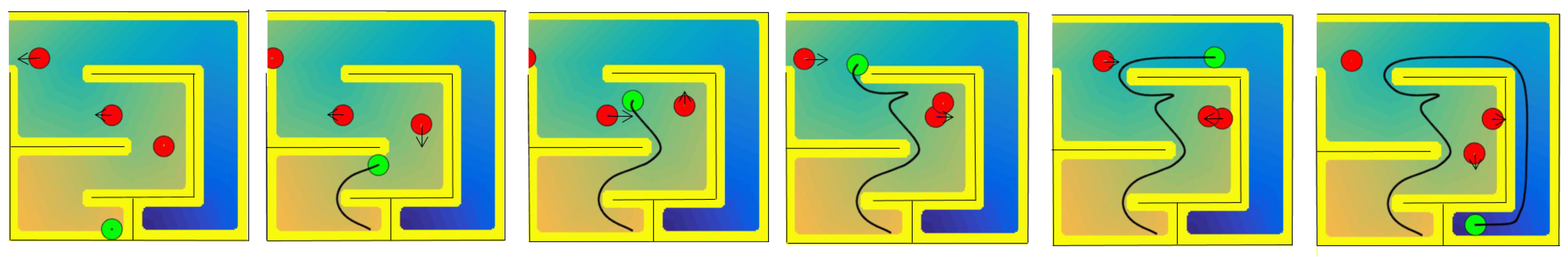
5.1. Avoiding Multiple Passive Agents

We will present the optimization procedure to navigate a robot among multiple passive agents, from a random start point to next (sub) goal $p_g$, in an open environment. This paper refers the goal as a point extracted from some global way point plan. For the considered environment, the algorithm should be able to quickly re-plan motion for an arbitrary starting point. Instead of conforming to any specific path, it requires the robot to avoid collision with passive agents while moving towards the goal. The proposed approach is based on computing optimal control input that brings robot closer to goal, while its margin should be greater than or equal to some allowable minimum safety margin, represented by $\beta$.

The control input $u_s^{*}$ that is actually given to a robot has margin greater than or equal to $\beta$, (14) and it minimizes the cost in (15) :

$$mrg(u_s^{*},U{O}^{\tau })\ge \beta$$

(14)

$$u_s^{*}=arg\underset{u_s\in U_{safe}^{\tau }}{min}\left|\right|f\left(h(x_a,u_s,\tau )\right)-p_g\left|\right|$$

(15)

That is, the navigation problem can be formulated as the problem of finding $u_s\in U_{safe}^{\tau }$ for which position $f\left(h(x_a,u,\tau )\right)$ is closest to $p_g$ in terms of Euclidean distance, and the margin $mrg(u_s^{*},U{O}^{\tau })$ is greater than or equal to minimum safety margin $\beta$. In case, if no control input in $U_{safe}^{\tau }$ satisfies (14) then control input with the biggest margin is selected, thus giving priority to safety. In this optimization problem, the interaction time horizon $\tau$ can be set equal to time horizon over which the behavior of obstacles is predicted, that is typically in the range of 3 to 10 s. The computed control input is applied for a short time step unless a new control loop begins. It results in continuous sense-plan-act navigation framework. The rest of the section will present the procedure of solving the optimization problem.

Explicit construction of control obstacle and safe control space is computationally challenging. We can earn computational savings by adopting a sampling based optimization procedure. Algorithm 1 summarizes the procedure for obtaining a set of safe control inputs and a set of inputs in the control obstacle. The sampling function on line 4 generates uniformly distributed samples in admissible control space for simplicity. However, more intelligent sampling procedure can be used. Each sampled control input is tested against temporary control obstacle at discrete time steps to obtain a set of safe control inputs and a set of control inputs in the control obstacle.

Algorithm 1 Sample Control Space

1: $U_{safe}^{\tau }⟵\mathrm{⌀}$ 2: $U{O}^{\tau }⟵\mathrm{⌀}$ 3: for $i=0$ to n do 4:     $u_i⟵$ Sample($U_{ad})$ 5:     for $t=0:\delta t:\tau$ do 6:         if $u_i\in {\bigcup }_{j\in N}U{O}_j\left(t\right)$ then 7:            $U{O}^{\tau }=U{O}^{\tau }\bigcup u_i$ 8:            break loop 9:         end if 10:     end for 11:     if $u_i\notin U{O}^{\tau }$ then 12:          $U_{safe}^{\tau }=U_{safe}^{\tau }\bigcup u_i$ 13:     end if 14: end for

Algorithm 2 summarizes the procedure used for selecting a best safe control input to be given to a robot. A sampling based margin of $u_s$ can be computed, which will be the weighted Euclidean distance of $u_s$ to the nearest sampled control input within control obstacle. It is the overestimate of the actual margin, as shown in Figure 4. Margin function on line 4 returns overestimated margin if it is less than $\beta$, else it returns $\beta$ as the margin of tested control input. For computing margin of $u_s$, only those samples are visited that are within a distance $\beta$ from $u_s$ in control space. In line 6, the function $max\left(m\right)$ returns largest margin found for the tested control inputs. Lines 7 to 17 mention the procedure of finding control input, that minimize the cost given in (15), and have overestimated margin greater than or equal to $\beta$. If all the tested control inputs have margin less than $\beta$ then the one with the biggest margin is returned.

Algorithm 2 Find Best Safe Control Input

1: $\beta ⟵$ minimum margin for inputs 2: $min⟵\infty$ 3: for all $u_i\in U_{safe}^{\tau }$ do 4:     $m\left[i\right]⟵mrg(u_i,U{O}^{\tau },\beta )$ 5: end for 6: $m_a=m_b=max\left(m\right)$ 7: if $max\left(m\right)\ge \beta$ then 8:     $m_a=max\left(m\right);m_b=\beta$ 9: end if 10: for all $u_i\in U_{safe}^{\tau }$ do 11:     if $m\left[i\right]\in [m_a,m_b]$ then 12:         if $\left|\right|f(h(x_a,u_i,\tau )-p_g)\left)\right||<min$ then 13:            $min⟵\left|\right|f(h(x_a,u_i,\tau )-p_g)\left|\right|$ 14:            $argmin⟵u_i$ 15:         end if 16:     end if 17: end for

5.2. Global Navigation

As other VO based approaches, the above presented approach is also subjected to a local minimum in the vicinity of large static concave obstacles. In such environment, the proposed framework can be incorporated into a global navigation plan. The key insight is that the admissible control space represents system compliant trajectories. By considering these trajectories up to time horizon $\tau$, a tree of depth one can be obtained. This tree can be searched and expanded based on margin of segments using a graph search method as one presented in [28]. During the search, all those segments that lie in control obstacle or are in collision with a static obstacle are considered as forbidden control inputs and are discarded. By running these components in a loop, a model predictive partial motion planning framework is obtained.

6. Implementation and Results

The previous sections have presented the framework of defining safe control space for a generalized agent dynamics. This section applies the framework to two types of kinodynamic model of the robot, namely the double integrator, and a car-like robot. Further, this section evaluates the performance of the proposed navigational approach for different parameters and presents its comparison with current approaches.

6.1. Considered Kinodynamic Model of Robot

6.1.1. Car-Like Robot

As illustrated in Figure 2, the states of the car-like robot can be given by the center position of the rear wheel axle $p_a={\left[x_a{y}_a\right]}^T$, its orientation $\theta$ and steering angle $\varphi$. Its state-transition equations are given by:

$${\dot{x}}_a\left(t\right)=v_{s}cos\theta \left(t\right)$$

$${\dot{y}}_a\left(t\right)=v_{s}sin\theta \left(t\right)$$

(16)

$$\dot{\theta }\left(t\right)=v_{s}k$$

where $v_s$ is the speed control input, k is the curvature control input. As in [26], curvature is directly taken as a control input, and the steering angle $\varphi$ is computed as $\varphi ={tan}^{-1}\left(kL\right)$ , where L represents the wheelbase of the car. We will denote the control input vector ${\left[v_{s}k\right]}^T$ by u. The states of the car-like robot are constrained as follow:

$$\sqrt{{\dot{x}}_a{\left(t\right)}^2+{\dot{y}}_a{\left(t\right)}^2}\in [0,v_m]$$

(17)

$$\dot{\theta }\left(t\right)/\sqrt{{\dot{x}}_a{\left(t\right)}^2+{\dot{y}}_a{\left(t\right)}^2}\in [-k_m,k_m]$$

(18)

where $v_m$ and $k_m$ are the maximum velocity and curvature constraints on robot states, respectively. For these constraint, $U_{ad}$ will be a rectangular region in control space such that $\left|k\right|<k_m$ and $|v_s|<v_m$. The expression for the position of the robot at a time t is obtained by integrating (16) under the assumption that the control inputs will remain constant over the time horizon t, and it is given as follows:

• if $k\ne 0$,

  $$\begin{array}{c}{p}_a(t,u)=p_a+R\left({\theta }_a\right)\ast \frac{1}{k}\left[\begin{array}{c}sin\left(v_{s}kt\right)\\ 1-cos\left(v_{s}kt\right)\end{array}\right]\hfill \\ \hfill \end{array}$$

  (19)
• if $k=0$,

  $$\begin{array}{c}\hfill p_a(t,u)=p_a\left(0\right)+R\left({\theta }_a\right){\left[t{v}_{s}0\right]}^T\\ \hfill \end{array}$$

  (20)

where $p_a$ and ${\theta }_a$ are the current position and orientation of the robot, respectively and $R\left({\theta }_a\right)$ is a rotation matrix equal to ($cos{\theta }_a-sin{\theta }_a;sin{\theta }_{a}cos{\theta }_a$).

6.1.2. Double Integrator

Consider a robot with dynamics as of double integrator and its states are constrained as follows:

$$\begin{array}{c}\hfill \sqrt{{\dot{x}}_a{\left(t\right)}^2+{\dot{y}}_a{\left(t\right)}^2}\in [0,v_m]\end{array}$$

(21)

$$\begin{array}{c}\hfill \sqrt{{\ddot{x}}_a{\left(t\right)}^2+{\ddot{y}}_a{\left(t\right)}^2}\in [0,a_m]\end{array}$$

(22)

where $v_m$ and $a_m$ are the maximum velocity and acceleration constraints of robot, respectively. Similar to work in [23], we let the robot to choose a velocity u instead of acceleration. Due to constraints on its states, the new velocity cannot be adopted instantaneously. A proportional control for acceleration is used for the robot, that is the acceleration applied at time t is equal to the difference between new velocity u and velocity ${\dot{p}}_a\left(t\right)$ at that time.

$$\begin{array}{c}\hfill {\ddot{p}}_a(t,u)=\frac{u-{\dot{p}}_a\left(t\right)}{\eta }\end{array}$$

(23)

where $\eta$ is a control parameter whose unit is time. By integrating (23) we obtain:

$$\begin{array}{c}\hfill {\dot{p}}_a(t,u)=u-e^{-t/\eta }(u-{\dot{p}}_a\left(0\right))\end{array}$$

(24)

where ${\dot{p}}_a\left(0\right)$ is the current velocity of the robot. By integrating (24) we obtain:

$$\begin{array}{c}\hfill p_a(t,u)=p_a\left(0\right)+tu+\eta (e^{-t/\eta }-1)(u-{\dot{p}}_a\left(0\right))\end{array}$$

(25)

where $p_a\left(0\right)$ is the current position of a robot. The admissible velocities space due to acceleration constraints is a disc in velocity space, its radius is equal to $\eta a_m$ and its center is at ${\dot{p}}_a\left(0\right)$. The admissible velocities space due to speed constraints is a disc in velocity space, its radius is equal to $v_m$ and its center is at the origin. The intersection of these two convex spaces will give us an admissible velocity space $U_{ad}$.

6.2. Implementation Details and Simulation Setup

This section will describe the implementation of the proposed algorithm and discuss its performance based on a set of simulated experiments. The experiments are conducted for a car-like robot and a double integrator, governed by the kinodynamic model described in Section 6.1. For each experiment, the interaction time horizon $\tau$ is set to $3.5$ s. The weighted matrix M defined in Definition 04 is set to identity matrix. The following constraints are considered on robot states in the simulations:

• Car-like robot: Maximum velocity $v_m=1.5$ unit/s, Maximum curvature $k_m=1.5$ unit ${}^{-1}$.
• Double integrator: Maximum velocity $v_m=2$ unit/s, Maximum acceleration $a_m=1$ unit/$s^2$.

The algorithm is implemented in C++, on a computer running Windows 10. The timing results are generated on Intel i5-3550 PC with 4-GB RAM. Although it is possible to build $U_{safe}^{\tau }$ and $U{O}^{\tau }$ using multiple cores, we use single-core to produce timing results.

Figure 5 shows the trajectory undertaken by the car-like robot to reach the goal while avoiding a collision with a static passive agent for different selected $\beta$. Figure 6 shows the same for the double integrator.

6.3. Collision Avoidance with Multiple Passive Agents

Each experiment is conducted in an open environment. Robot initial position is set to $(5,10)$, and it has to move towards a goal at $(20,20)$. Several circular obstacles representing passive agents are randomly distributed in a square region bounded by $(0,0)$ and $(22,22)$. All passive agents and robot have radii equal to 1 unit. Similar to [26], passive agents are assigned arbitrary velocities and the maximum upper limit on their speeds is set to $\pm 1$ unit/s. The probability that the passive agent will change its velocity within 1 s is $0.2$. Figure 7 shows multiple snapshots at different time instances of the car-like robot, in green, avoiding collision with multiple passive agents, in red, while moving towards the goal marked in yellow.

An empirical test showing the performance of the algorithm is presented in the following subsections, where each experimental value is the mean of 10 trials.

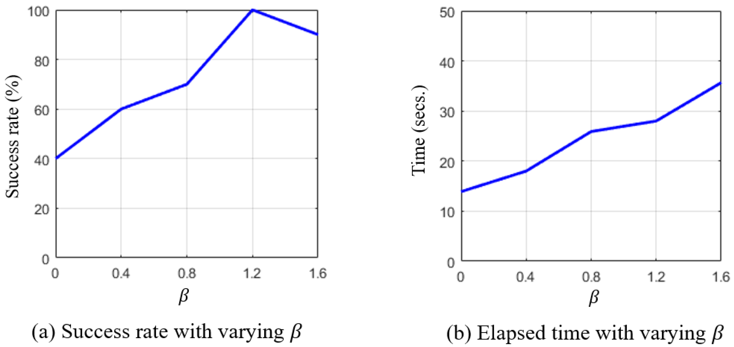
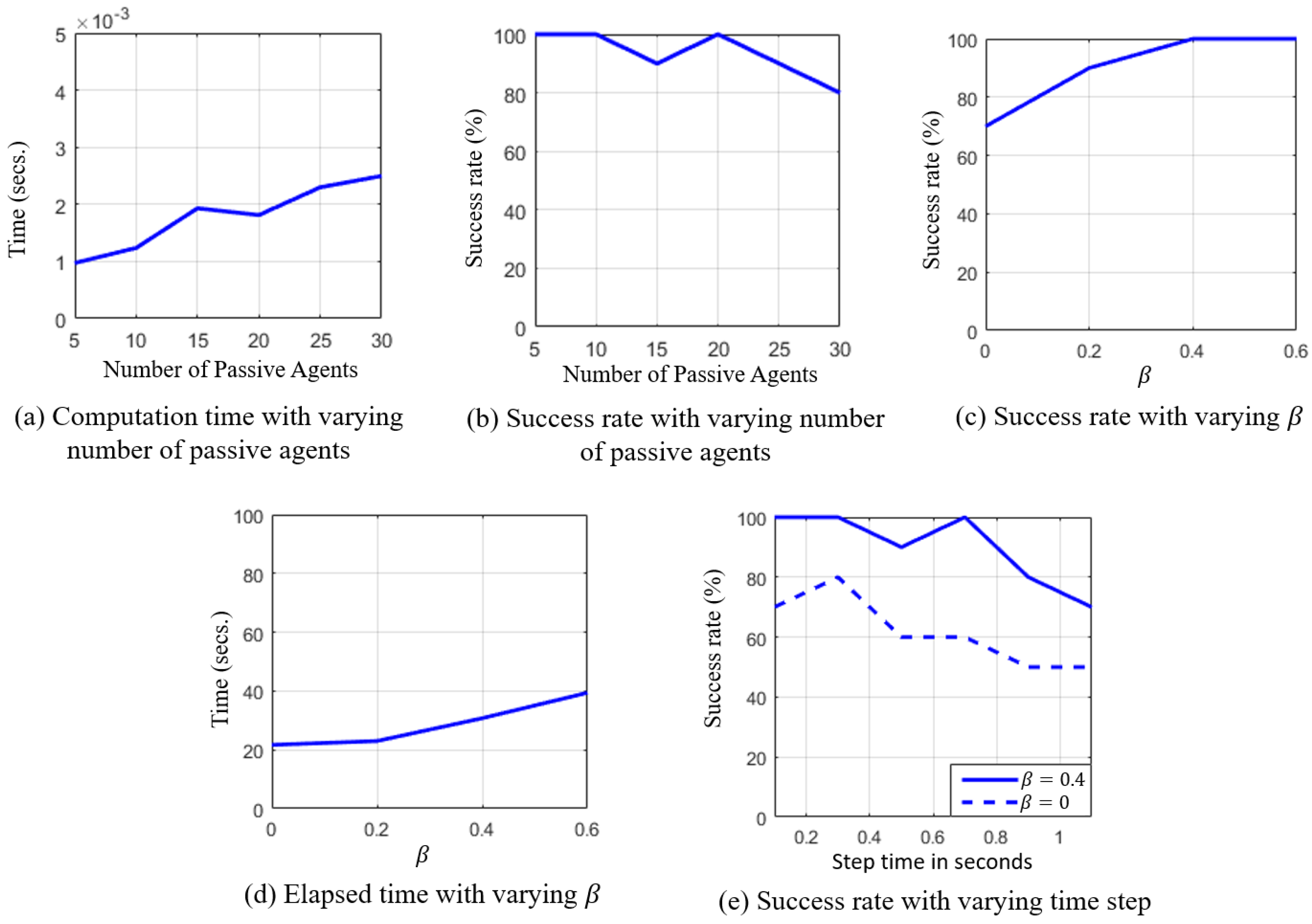
6.3.1. Performance Results

In Figure 8, the performance of the proposed algorithm for a car-like agent is presented for the set of three parameters, the number of passive agents present, minimum saftey margin $\beta$, and the length of the time step. The effect on computation time, success rate, and elapsed time are investigated. The computation time is the time required to compute optimal control input. A successful run is a trial in which agent successfully reaches the goal without a collision. A collision might occur when a passive agent changes its direction and traps the robot. In a successful trial, elapsed time is the amount of time passed, starting from the point in time when the robot was at its initial position, to the point in time when robot reaches the goal position. Figure 8a shows an average computation time taken when the number of obstacles present grows. The computation time increases approximately linearly with the increase in a number of passive agents, while Figure 8b shows the success rate drops with the growth in the number of passive agents. For these experiments the step time was set to 5 ms, the margin was set to 0.4, and 256 samples was taken in $U_{ad}$. In Figure 8c, the success rate is shown for selected values of $\beta$, when 20 passive agents are present. It shows that the success rate increases with the increase in $\beta$, while Figure 8d shows that the elapsed time also increases with the increase in $\beta$. For larger value of $\beta$, the robot takes comparatively longer time to reach the goal because it selects a more safe path to the goal rather than a direct path to it. Finally, Figure 8e shows the success rate when $\beta$ is set equal to 0, and $0.4$, for varying step time. It shows that the increase in step time will lead to a drop in success rate, whereas the success rate is comparatively higher for $\beta =0.4$ than that for $\beta =0$.

The results in Figure 8c,d show that the car-like robot reaches the goal with relatively high success rate when $\beta$ = 0.4 is selected, while the elapsed time is comparatively reasonable. The next subsection will compare the performance of the proposed approach ($U_{safe}$) with $\beta =0.4$ to that of GVO.

6.3.2. Comparison with GVO

In Figure 9, a comparison of performance is shown for the proposed $U_{safe}$ approach and GVO approach. The comparison is made regarding the effect on computation time, success rate, and elapsed time, for varying number of passive agents present. In this comparison 256 control inputs are sampled in admissible control space. In Figure 9, (a) shows average computation time for the two approaches, where computation time for GVO is much higher compared to $U_{safe}$. (b) shows the comparison of average success rate. The success rate of GVO is much lower compared to $U_{safe}$, as for GVO approach the robot is frequently trapped by the passive agents. Finally, Figure 9c compares the elapsed time for the two approaches. For $U_{safe}$, the robot takes a safer path rather than a direct path to reach the goal. Thus, the robot takes a comparatively longer time to reach the goal. In summary, we can conclude that the performance of $U_{safe}$ is much better than GVO.

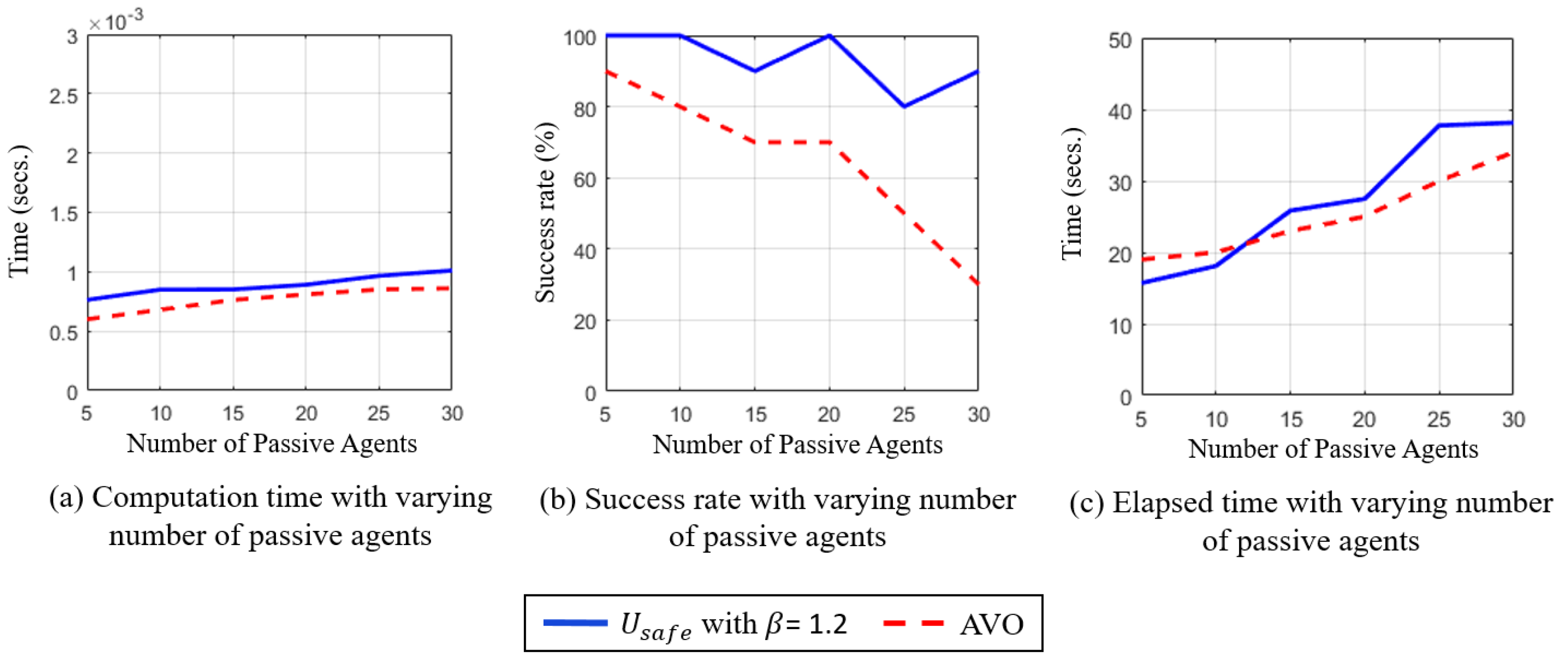
6.3.3. Comparison with AVO

In order to make a comparison with AVO [23], the robot with kinodynamic model as of double integrator is considered. We have modified AVO by removing its reciprocal collision avoidance aspect and keeping the linear programming optimization. The control parameter $\eta$ is set to 3 for these experiments. For $U_{safe}$, $\beta$ is set to 1.2. The graphs in Figure 10 presents the performance of proposed $U_{safe}$ approach for selected values of $\beta$. The experiment results in Figure 11 show the performance of AVO algorithm and the proposed $U_{safe}$ approach. It shows the effect on average computation time, success rate, and time elapsed, against varying number of passive agents. In Figure 11, (a) shows the average computation time for the two approaches, where AVO takes slightly lesser time on average for computing the solution. (b) shows the comparison of average success rate, the success rate for AVO is much lower as compared to $U_{safe}$. (c) shows that the elapsed time is almost same for the two approaches.

Under AVO approach, the velocity obstacle induced due to each passive agent is approximated by a half plane in velocity space, this leads to a computed collision free control space which is frequently empty, thus give rise to the number of the failures in computing the solution.

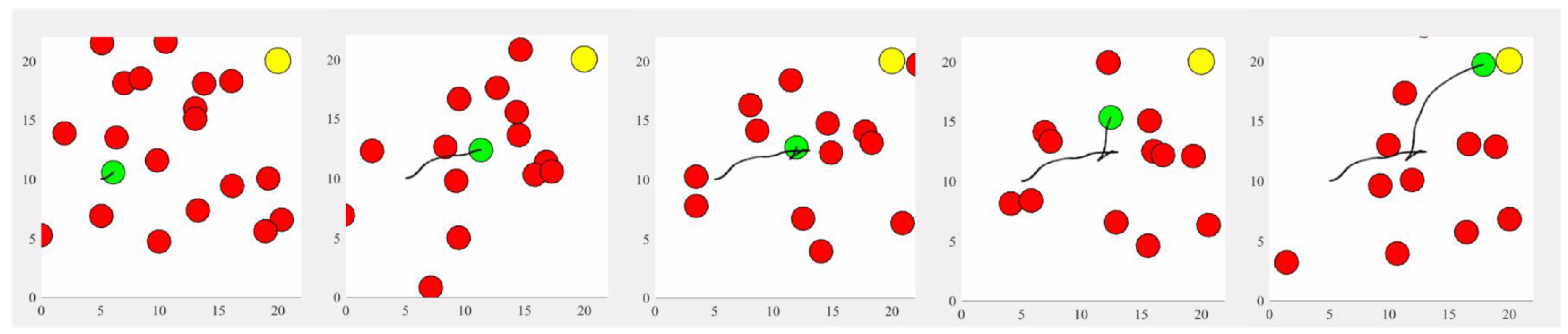
6.4. Global Navigation

The real world environment usually has static obstacles in addition to passive agents. These static obstacles are usually concave, and the VO based approaches are subjected to a local minimum in such environments. The presented concept of safe control space allows us to integrate the control space in a graph search fashion. Figure 12 shows the framework where multiple snapshots at different time instances are shown. In this simulation, the interaction time horizon $\tau$ is set to 4 s and 256 control inputs are sampled in an admissible control space. All samples that lie in the control obstacle or collide with static obstacles are discarded to obtain a tree depth of one. In this experiment, the graph search terminates at the depth of one, the point at which $f\left(h(x_a,u,\tau )\right)$ connects to Dijkstra heuristic function. The trajectory that is executed for one control cycle is the one that minimize the Dijkstra heuristic function and has a margin greater than or equal to $1.2$. As a result, we obtain a global optimization criteria for navigating the agent. However, in case if all tested samples has margin less then $\beta$, than the sample with the biggest margin is selected.

7. Conclusions

This paper presented a fast navigation approach for a dynamic environment where the behavior of passive agents is partially predictable. The concept of safe control space is presented by generalizing the nonlinear velocity obstacle, which makes it possible to consider the robot model for computing the system compliant collision-free trajectories. The safety margin defined for safe control inputs allows the robot to make a safe decision in the environment where the predicted trajectories of passive agents change frequently. The ability of the proposed algorithm to compute a safe decision in real-time is demonstrated. The comparative study validates that under the proposed approach the robot reaches the goal with high success rate. The proposed approach can be incorporated into a waypoint plan for global navigation. One possible implementation of a global navigation plan is presented in the paper.

In future, authors will attempt the problem of dynamically adapting the minimum safety margin parameter based on the circumstances. Also, an interesting direction for future work will be the extension of the proposed approach to the environment with multiple active and passive agents. In addition to this, the authors are interested in planning for situations with dynamic obstacles have deterministic behavior.

References

1. Prassler, E.; Scholz, J.; Fiorini, P. A robotic wheelchair for crowded public environments. IEEE Robot. Autom. Mag. 2001, 8, 38–45. [Google Scholar]
2. Breitenmoser, A.; Tâche, F.; Caprari, G.; Siegwart, R.; Moser, R. MagneBike: Toward multi climbing robots for power plant inspection. In Proceedings of the 9th International Conference on Autonomous Agents and Multiagent Systems: Industry track, Toronto, ON, Canada, 10–14 May 2010; International Foundation for Autonomous Agents and Multiagent Systems: Singapore, 2010; pp. 1713–1720. [Google Scholar]
3. Laumond, J.P.; Jacobs, P.; Taïx, M.; Murray, R. A Motion Planner for Nonholonomic Mobile Robots. IEEE Trans. Robot. Autom. 1994, 10, 577–593. [Google Scholar]
4. Scheuer, A.; Fraichard, T. Continuous-curvature path planning for car-like vehicles. In Proceedings of the IEEE International Conference on Intelligent Robots and Systems, Grenoble, France, 7–11 September 1997; Volume 2, pp. 997–1003. [Google Scholar]
5. Lamiraux, F.; Laumond, J.P. Smooth motion planning for car-like vehicles. IEEE Trans. Robot. Autom. 2001, 17, 498–502. [Google Scholar]
6. Frazzoli, E.; Dahleh, M.; Feron, E. Real-time motion planning for agile autonomous vehicles. J. Guid. Control Dyn. 2002, 25, 116–129. [Google Scholar]
7. Hsu, D.; Kindel, R.; Latombe, J.C.; Rock, S. Randomized kinodynamic motion planning with moving obstacles. Int. J. Robot. Res. 2002, 21, 233–255. [Google Scholar]
8. Zucker, M.; Kuffner, J.; Branicky, M. Multipartite RRTs for rapid replanning in dynamic environments. In Proceedings of the IEEE International Conference on Robotics and Automation, Roma, Italy, 10–14 April 2007; pp. 1603–1609. [Google Scholar]
9. Kant, K.; Zucker, S. Toward Efficient Trajectory Planning: The Path-Velocity Decomposition. Int. J. Robot. Res. 1986, 5, 72–89. [Google Scholar] [CrossRef]
10. Peng, J.; Akella, S. Coordinating multiple Robots with kinodynamic constraints along specified paths. Int. J. Robot. Res. 2005, 24, 295–310. [Google Scholar] [CrossRef]
11. Van Den Berg, J.; Overmars, M. Kinodynamic motion planning on roadmaps in dynamic environments. In Proceedings of the IEEE International Conference on Intelligent Robots and Systems, San Diego, CA, USA, 29 Octomber–2 November 2007; pp. 4253–4258. [Google Scholar]
12. Gaillard, F.; Soulignac, M.; Dinont, C.; Mathieu, P. Deterministic kinodynamic planning with hardware demonstrations. In Proceedings of the IEEE/RSJ International Conference on Intelligent Robots and Systems (IROS), San Francisco, CA, USA, 25–30 September 2011; pp. 3519–3525. [Google Scholar]
13. Chen, C.; Rickert, M.; Knoll, A. Kinodynamic motion planning with space-time exploration guided heuristic search for car-like robots in dynamic environments. In Proceedings of the IEEE/RSJ International Conference Intelligent Robots and Systems (IROS), Hamburg, Germany, 28 September–2 Octomber 2015; pp. 2666–2671. [Google Scholar]
14. Bennewitz, M.; Burgard, W.; Thrun, S. Learning motion patterns of persons for mobile service robots. In Proceedings of the IEEE International Conference on Robotics and Automation, Washington, DC, USA, 11–15 May 2002; Volume 4, pp. 3601–3606. [Google Scholar]
15. Vasquez, D.; Fraichard, T. Motion prediction for moving objects: A statistical approach. In Proceedings of the IEEE International Conference on Robotics and Automation, New Orleans, LA, USA, 26 April–1 May 2004; Volume 4, pp. 3931–3936. [Google Scholar]
16. Kim, S.; Guy, S.; Liu, W.; Wilkie, D.; Lau, R.; Lin, M.; Manocha, D. BRVO: Predicting pedestrian trajectories using velocity-space reasoning. Int. J. Robot. Res. 2015, 34, 201–217. [Google Scholar] [CrossRef]
17. Bera, A.; Kim, S.; Randhavane, T.; Pratapa, S.; Manocha, D. GLMP-realtime pedestrian path prediction using global and local movement patterns. In Proceedings of the IEEE International Conference on Robotics and Automation (ICRA), Stockholm, Sweden, 16–21 May 2016; pp. 5528–5535. [Google Scholar]
18. Fiorini, P.; Shiller, Z. Motion planning in dynamic environments using velocity obstacles. Int. J. Robot. Res. 1998, 17, 760–772. [Google Scholar] [CrossRef]
19. Van Den Berg, J.; Guy, S.J.; Lin, M.; Manocha, D. Reciprocal n-body collision avoidance. In Robotics Research; Pradalier, C., Siegwart, R., Hirzinger, G., Eds.; Springer: Berlin, Germany, 2011; pp. 3–19. [Google Scholar]
20. Best, A.; Narang, S.; Manocha, D. Real-time reciprocal collision avoidance with elliptical agents. In Proceedings of the IEEE International Conference on Robotics and Automation (ICRA), Stockholm, Sweden, 16–21 May 2016; pp. 298–305. [Google Scholar]
21. Alonso-Mora, J.; Breitenmoser, A.; Rufli, M.; Beardsley, P.; Siegwart, R. Optimal reciprocal collision avoidance for multiple non-holonomic robots. In Distributed Autonomous Robotic Systems; Springer: Berlin, Germany, 2013; pp. 203–216. [Google Scholar]
22. Alonso-Mora, J.; Breitenmoser, A.; Beardsley, P.; Siegwart, R. Reciprocal collision avoidance for multiple car-like robots. In Proceedings of the IEEE International Conference on Robotics and Automation (ICRA), Saint Paul, MN, USA, 14–18 May 2012; pp. 360–366. [Google Scholar]
23. Van Den Berg, J.; Snape, J.; Guy, S.J.; Manocha, D. Reciprocal collision avoidance with acceleration-velocity obstacles. In Proceedings of the IEEE International Conference on Robotics and Automation (ICRA), Shanghai, China, 9–13 May 2011; pp. 3475–3482. [Google Scholar]
24. Rufli, M.; Alonso-Mora, J.; Siegwart, R. Reciprocal collision avoidance with motion continuity constraints. IEEE Trans. Robot. 2013, 29, 899–912. [Google Scholar] [CrossRef]
25. Bareiss, D.; Van Den Berg, J. Generalized reciprocal collision avoidance. Int. J. Robot. Res. 2015, 34, 1501–1514. [Google Scholar] [CrossRef]
26. Wilkie, D.; Van Den Berg, J.; Manocha, D. Generalized velocity obstacles. In Proceedings of the IEEE/RSJ International Conference on Intelligent Robots and Systems (IROS), St. Louis, MO, USA, 10–15 October 2009; pp. 5573–5578. [Google Scholar]
27. Shiller, Z.; Large, F.; Sekhavat, S. Motion planning in dynamic environments: Obstacles moving along arbitrary trajectories. In Proceedings of the IEEE International Conference on Robotics and Automation, Seoul, Korea, 21–26 May 2001; Volume 4, pp. 3716–3721. [Google Scholar]
28. Park, J.; Iagnemma, K. Sampling-based planning for maximum margin input space obstacle avoidance. In Proceedings of the IEEE/RSJ International Conference on Intelligent Robots and Systems (IROS), Hamburg, Germany, 28 September–2 Octomber 2015; pp. 2064–2071. [Google Scholar]
Figure 1. For a robot with current position p a ( 0 ) at origin and obstacle following trajectory c ( t ) , (a) shows the temporary velocity obstacle, N L V O ( t i + n ) induced for a robot due to the position of an obstacle at time t i + n . It is a disc of radius ( r a + r b ) / t i + n and its center is at c ( t i + n ) / t i + n in the robot velocity space. If the velocity of a robot is such that v a N L V O ( t i + n ) , then p a ( t i + n ) c ( t i + n ) B . In (b), N L V O τ is shown as the union of its temporary components over time horizon [ 0 , τ ] . If a robot velocity v a is in N L V O τ , then the collision will occur within time horizon [ 0 , τ ] . NLVO: Nonlinear Velocity Obstacle.
Applsci 07 00903 g001
Figure 2. Kinematic model of the car-like robot. States are given by the center position of rear wheel axle p a , the orientation angle θ , the steering angle ϕ . L represents the wheelbase of the car. Robot velocity v is in the direction of rear wheels. ICR: Instantaneous Center of Rotation.
Applsci 07 00903 g002
Figure 3. The green region in (a) is a safe control space U s a f e τ = 5 obtained by taking the complement of control obstacle U O τ = 5 in U a d . In (b), the paths undertaken by a robot for selected control inputs in U s a f e τ = 5 are shown. The velocity in red lies is in control obstacle and its associated path leads robot to penetrate into obstacle within 5 s. Velocity in yellow lies on the boundary of control obstacle thus, have margin zero. It leads the robot to graze the obstacle within 5 s. Velocity in blue has margin greater than zero and it leads the robot to navigate from a distance to the obstacle.
Applsci 07 00903 g003
Figure 4. A sampling-based estimate of u s margin , m r g ( u s , U O τ ) is the weighted Euclidean distance of u s to the nearest tested control in control obstacle. It is the overestimate of actual margin of u s .
Applsci 07 00903 g004
Figure 5. It shows the paths taken by a car-like robot to reach the goal at (20,10) from its initial position at (5,10), for selected β , while avoiding collision with a static passive agent at (12,9).
Applsci 07 00903 g005
Figure 6. It shows the paths taken by a double integrator to reach the goal at (20,10) from its initial position at (5,10), for selected β , while avoiding collision with a static passive agent at (12,9). The control parameter η was set to 3.
Applsci 07 00903 g006
Figure 7. Avoiding multiple passive agents. Multiple snapshots at different time instances show a car-like robot, in green, navigates among multiple passive agents, in red, while moving towards a goal p g , in yellow. The passive agents are moving with arbitrary velocities. The probability that a passive agent will change its velocity within one second is 0.2. { β = 0 . 4 is set for the simulation}.
Applsci 07 00903 g007
Figure 8. In this graph, the performance of the proposed algorithm for a car-like robot is presented for the set of three parameters, the number of passive agents present, minimum saftey margin β , and the length of the time step. The effects on computation time, success rate, and elapsed time, are shown.
Applsci 07 00903 g008
Figure 9. It shows the performance of GVO algorithm and the proposed U s a f e approach. The effect on average computation time, success rate, and elapsed time, are shown against varying number of passive agents. GVO: Generalized Velocity Obstacle.
Applsci 07 00903 g009
Figure 10. In this graph, the performance of the proposed algorithm U s a f e for double integrator is presented for the scenario when 20 passive agents are present. (a) show the success rate for selected values of β . (b) show the elapsed time for different values of β . The robot takes comparatively longer time to reach goal when the larger value for β is set, as robot take the safer path to the goal rather than a direct path to it. Results show that robot reaches the goal with relatively high success rate when β = 1.2 is selected, while the elapsed time is comparatively reasonable.
Applsci 07 00903 g010
Figure 11. It shows the performance of AVO algorithm and the proposed U s a f e approach. The effect on average computation time, success rate, and elapsed time, are shown against varying number of passive agents. AVO: Acceleration-Velocity Obstacle.
Applsci 07 00903 g011
Figure 12. Global navigation plan. Robot employs a heuristic graph search strategy. The color gradient shows the Dijkstra heuristic field for the maze. The interaction horizon is τ = 4 s. The safe control inputs are computed, which are neither in control obstacle nor did they lead to a collision with the static obstacle. At the same time, Dijkstra heuristic function computes the cost for reaching the goal. A safe control input is executed which minimizes the cost and has margin greater than or equal to β = 1 . 2 .
Applsci 07 00903 g012