Review

Machine Learning Methods for Pipeline Surveillance Systems Based on Distributed Acoustic Sensing: A Review

by
Javier Tejedor
1,
Javier Macias-Guarasa
2,*,
Hugo F. Martins
3,
Juan Pastor-Graells
2,
Pedro Corredera
4 and
Sonia Martin-Lopez
2
1
Department of Information Technology, University CEU San Pablo, 28003 Madrid, Spain
2
Department of Electronics, University of Alcalá, 28801 Alcalá de Henares, Spain
3
FOCUS S.L., 28004 Madrid, Spain
4
Instituto de Óptica, CSIC, 28006 Madrid, Spain
*
Author to whom correspondence should be addressed.
Appl. Sci. 2017, 7(8), 841; https://doi.org/10.3390/app7080841
Submission received: 19 July 2017 / Revised: 7 August 2017 / Accepted: 10 August 2017 / Published: 16 August 2017
(This article belongs to the Special Issue Distributed Optical Fiber Sensors)

Abstract

:
There is an increasing interest in researchers and companies on the combination of Distributed Acoustic Sensing (DAS) and a Pattern Recognition System (PRS) to detect and classify potentially dangerous events that occur in areas above fiber optic cables deployed along active pipelines, aiming to construct pipeline surveillance systems. This paper presents a review of the literature in what respect to machine learning techniques applied to pipeline surveillance systems based on DAS+PRS (although its scope can also be extended to any other environment in which DAS+PRS strategies are to be used). To do so, we describe the fundamentals of the machine learning approaches when applied to DAS systems, and also do a detailed literature review of the main contributions on this topic. Additionally, this paper addresses the most common issues related to real field deployment and evaluation of DAS+PRS for pipeline threat monitoring, and intends to provide useful insights and recommendations in what respect to the design of such systems. The literature review concludes that a real field deployment of a PRS based on DAS technology is still a challenging area of research, far from being fully solved.

1. Introduction

The most sustainable and safest transmission method to transport energy sources from the producing facilities to the various end-users relies on pipeline transmission. In this environment, pipeline integrity is crucial for a safe operation, and must be specially pursued when crossing urban areas. Despite all safeguard measures taken by the system operators, zero risk does not exist, being the energy transmission an industrial activity, so that extra care must be taken to avoid the pipeline to be damaged. This is especially important if we take into account that most incidents involving natural gas transmission infrastructures occur due to external interference (between 50% and 60% of the reported incidents according to [1,2], well above the second main cause (construction defect or material failure, which account for between 16% and 25% of the cases, respectively)), mainly due to third party works in the pipeline vicinity, some of which unfortunately lead to human casualties. In addition to personal losses, the incidents leading to interruption of energy supply and leaked fuel associated also derive in high economic losses (as a consequence of supply disruption) and environmental damage. To provide an example, as reported in [2], between 1984 and 2004, the documented incidents in natural gas distribution pipelines in the United States (2842) led to a property damage value of over 323 million dollars, with 337 fatalities and 1525 injured people.
The security of pipelines has significantly improved, but there is still a high demand for high-performance and cost-effective solutions for continuous monitoring potential threats to the integrity of pipelines. Given the length and linearity of the transmission pipelines, often spanning hundreds of kilometers, distributed acoustic sensing (DAS) technology is specially well suited for this task [3,4,5,6,7,8,9,10,11], as it allows monitoring large distances with a single interrogation unit. The fact that deployment of fiber optic bundles when building pipelines is a routine well established action, also contributes to the feasibility of DAS-based pipeline integrity monitoring systems.
Distributed acoustic sensors are able to detect vibrations that occur on the ground nearby the top of a buried optical fiber deployed along a pipeline, and hence monitor activities near it. This represents a promising solution as the vibrations associated to potentially dangerous activities can be detected, so that a preventive action can be undertaken. If machine learning strategies are employed to develop a pattern recognition system (PRS) that can further classify the sensed vibration into a set of relevant activities, we can increase the cost-effectiveness of the system, as the provided information will be richer, and the number of false alarms can be significantly reduced.
Although some works have been presented in this direction [3,12,13,14,15,16,17,18,19,20,21,22,23,24,25,26,27], there is still, many times, a lack of understanding of how a reliable and efficient system can be built, and what is the adequate and rigorous methodology to apply in the system evaluation processes. In addition, to the best of our knowledge, no thorough written report that summarizes the main characteristics of these systems exists in the literature applied to DAS+PRS technology. So, the purpose of this paper is two-fold:
  • Present the first extensive review of the machine learning techniques applied on DAS-based surveillance systems.
  • Provide meaningful recommendations for a methodology that aims to build a DAS-based surveillance system based on machine learning techniques.
We want also to stress the fact that even when the paper focuses on the application of pipeline monitoring, its scope and discussion can also be applied and extended to any other environment or structure in which DAS+PRS technology is to be used.
The rest of the paper is organized as follows: Section 2 presents some previous works on DAS, and works related to machine/vehicle classification that employ other sensors rather than distributed acoustic ones. Section 3 presents the principles of the machine learning strategy applied to DAS. Section 4 presents a literature review of the published approaches employed for DAS+PRS, along with their results. Discussion of the corresponding approaches is presented in Section 5, and real field deployment system issues are presented in Section 6. Some practical recommendations for applying machine learning techniques on DAS are given in Section 7, and the paper is concluded in Section 8.

2. Related Work

2.1. Distributed Acoustic Sensing and Pattern Recognition Systems (DAS+PRS)

As described in [24], fiber optic distributed acoustic sensing with phase-sensitive optical time-domain reflectometer ( ϕ -OTDR) technology shows good performance for long perimeter monitorization aiming to detect potential threats or intruders on the ground [3,28,29,30,31], or vibration in general [4,32,33,34,35,36,37,38,39].
The high sensitivity of conventional ϕ -OTDR-based sensors, with sensing ranges in the order of tens of kilometers and spatial resolutions in the meter range, provides the possibility of detecting low energy activities, such as people walking over a buried fiber [3]. Sensing ranges above 100 km have also been demonstrated with the use of optical amplification [4,5,35,40]. Post-processing denoising methods have also been applied to improve the signal-to-noise ratio (SNR) and therefore the limits of detection [33,35,41,42].
Even though the information provided by DAS is very powerful, the current and future trends will undoubtedly make extensive use of it in combination with PRS and machine learning techniques, as a way to provide relevant, richer, and higher level information on the surveilled systems.
In 2016, the authors of [23] presented the first extensive reported work on a pipeline integrity threat detection and identification system that employed DAS+PRS and was rigorously evaluated on realistic field data, showing promising results in terms of accuracy, and thus its potential for real world applications. Their work was developed under a GERG (The European Gas Research Group) supported project titled PIT-STOP (Early Detection of Pipeline Integrity Threats using a SmarT Fiber-OPtic Surveillance System), which addressed three main targets:
  • The rigorous application of machine learning methods and methodologies to the area of pipeline integrity surveillance, using distributed acoustic sensing.
  • The generation of extensive, varied, and realistic field data, using real machinery carrying out real activities sensed by state-of-the-art DAS systems on optical fibers deployed along active gas pipelines.
  • The application of objective evaluation metrics on the realistic data, so that the results could provide a real perspective on the actual capabilities of the DAS+PRS in the real world.
Most of the ϕ -OTDR-based reported works relied and focused on directly measuring changes in the optical trace, or were based on applying simple threshold-based strategies on the trace energy to detect perturbations. However, there is an increasing interest of employing more advanced techniques on more and more challenging and realistic scenarios.
As described in [23], from the few works that actually employed PRS techniques, most of them exhibited relevant problems that did not allow to objectively assess the validity of their claims, or their extensibility to realistic field deployments.
In some of them, no real classification was conducted [17], or no classification results were reported [18,43]. In others, there were no details of the system description [30], there were no details on the classification strategy [26], or not enough details of the experimental procedure (training and testing conditions, recording protocol, etc.) were given [19,21,26,43].
A major and generalized problem relates to the data generation process, since this is, in most cases, far from a real field environment: either the sensing system is very close to the sensed area [3,17], or the sensed area is small [17,19,35]. In some cases, no real acquired signals are used, but only simulated data [4,5,19,33,35,40,41,42,44].
Some recent works present significant improvements over those previously reported, by generating recording environments with longer optical fibers (in the range of tens of kilometers), such as [45] (17 km), [21] (20 km),  [27] (24 km), [46] (50 km), and [26] (220 km), thus approaching the idea of a more realistic environment. Also, their experimental procedure is more rigorous [45,46], even applying cross-validation (CV) techniques [21]. However, some of them generate all the measurements from a single position [27,46], hence biasing the system to recognize the position instead of the real event, which we demonstrated in [23] that was a major issue when facing realistic environments. In addition, the number of tested signals in the latter two works is small, with no additional details regarding the actual recording durations.
Some companies also offer solutions for pipeline surveillance monitoring, although they do not usually provide any details on their strategies, nor objective data for evaluation. As an example, in [43], a gas leak detection system based on simple energy thresholding (i.e., not using any pattern recognition techniques), and a third party intrusion detection tool, which seems to employ some kind of classification based on neural networks, are presented. However, the number of classes involved in the system is not stated and no experiments nor performance results are described.

2.2. Machine/Vehicle Classification from Other Sensing Systems

To provide some contrast on works that aim to a similar target, and compared with the few works that have employed DAS for signal acquisition, significant research has been conducted regarding the general task of classifying different types of vehicles/machinery by employing other sensing systems. We include here some references in this area to quantify the state of the art results that can be expected in this related research scenario, in which various strategies for the design of the PRS (mainly feature extraction and classification) have been used [47,48,49,50,51,52,53,54,55,56,57,58,59,60,61]. Table 1 shows the main features of those signal classification systems, in terms of the sensing method, feature extraction, classification algorithm employed, classification task, and classification accuracy. All these works differ from the works that employ DAS in the fundamental fact that the sensing method is based on a linear and stable transduction mechanism between the vehicle physical effects (acoustic or seismic) and the acquired signal. On the contrary, in ϕ -OTDR-based systems, the transduction function will not be stationary as it will be heavily affected by environmental conditions, varying along time and location. This is specially relevant when the DAS system is based on amplitude measurements, which inherently imply a non-linear behavior, except for very small perturbations. This non-stationary (and in some cases non-linear) response, can be clearly observed by analyzing the signal resulting from the detection of pure vibration frequencies: the ϕ -OTDR-based recorded signal will include amplitude varying harmonics and sub-harmonics along with the original vibration frequency. The linear transduction mechanism of the sensing systems shown in Table 1 implies that the acquired signals will have a reasonably consistent behavior, thus providing a favorable scenario for the classification task.

2.3. Summary

Most of the works reported in the literature that combine DAS with PRS have severe limitations, mainly related to the facts that classification results were not presented, there was a lack of realistic experimental conditions, and the experimental approach and procedures were not rigorous (evaluation metrics, database building, signal acquisition, reduced distances, etc.). Additionally, we can find a lot of works in the literature that also aim to detect different events (machinery types in general, as well as possible threats), with sensing methods that are completely different in nature and characteristics to those used in DAS systems. From these related works, the DAS+PRS strategy could benefit by importing their methodologies and techniques (in what respect to feature extraction, classification methods, experimental design, etc.).

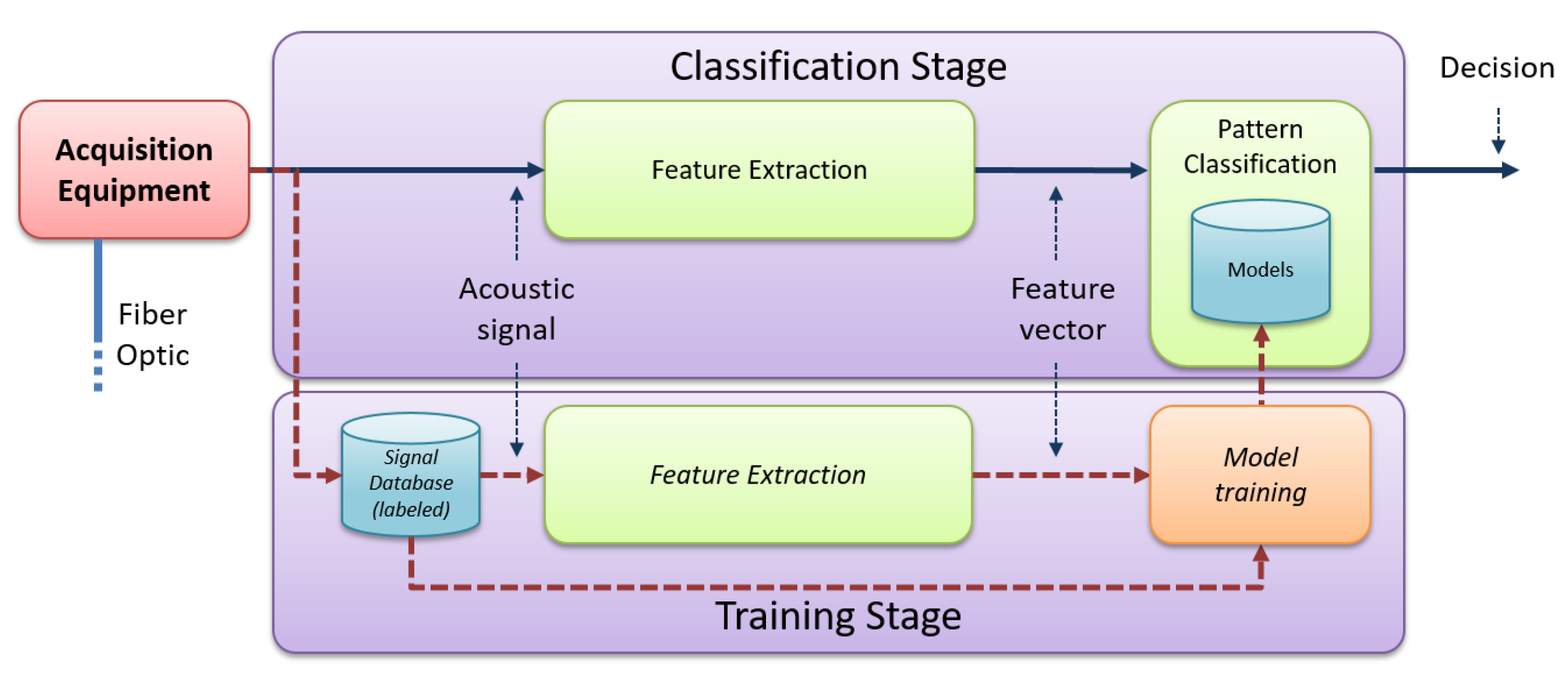
3. Principles of Machine Learning for DAS

3.1. Introduction

With the increasing amount of data in high-performance storage centers, machine learning technology provides a common framework for processing these data so that powerful and high level information aids in decision making processes. Many areas benefit from the application of this technology, such as general signal and text processing, speech processing, automatic translation, web page ranking, biometrics, risk analysis, anomaly detection, robotics, big data, etc. The distributed acoustic sensing area is rather novel, and can provide high quality data that are able to characterize physical effects in very long distances, and that needs to be further exploited to provide qualitative information on the actual causes of these physical effects.
Specifically, machine learning algorithms are employed to make predictions for unknown data sets from a previously set of data obtained in similar conditions. This set of data is typically employed to build statistical models that can then be used to make predictions.
The typical architecture of a simplified DAS+PRS is shown in Figure 1, where the Acquisition Equipment, connected to the fiber optic, is in charge of generating the acoustic signals that will be used for the training and classification stages (we refer to these signals as acoustic, considering that their frequency content in these sensing scenarios is in the audible range). The modules that comprise the Training Stage (in the lower part of Figure 1) are in charge of generating suitable models that accurately represent the input data characteristics for each of the considered classes. The Classification Stage modules (in the upper part of Figure 1) decide which of the trained models more accurately represent the input acoustic signals to generate a final decision. In both stages, the signal acquired is given to a feature extraction module, where meaningful patterns (feature vectors) are obtained. Next, the corresponding feature vectors (or sequence of vectors) are given to a pattern classification or training algorithm that classifies the feature vector as a certain class or is used to generate adequate models, depending on whether we are referring to the classification or training stages, respectively.

3.2. Feature Extraction

Feature extraction aims to extract meaningful and discriminative information from the raw acoustic signals recorded by the DAS system so that each different activity occurring at the top of the fiber can be next identified by the pattern classification module.
Feature extractors typically generate sequences of feature vectors x corresponding to the input signal, with components that are meant to be useful for the pattern classification task.
Features computed by the so-called feature extraction methods can be divided into three different categories: time domain features [62], frequency domain features [63], and time-frequency domain features [64]. The time domain features are suitable for non-stationary signals. Typically, these features comprise the energy of the signal, zero crossing rate (ZCR), correlation, auto-correlation, and Singular Spectrum Analysis (SSA), among others. The frequency domain features comprise spectrum-derived features, Fast Fourier Transform (FFT)-based features, formant/harmonic frequency-based features, Power Spectral Density (PSD), and Harmonic Line Association (HLA), among others. These frequency-based features are especially suitable for stationary or quasi-stationary signals. The time-frequency domain features try to get advantage of the time and frequency domains simultaneously, such as wavelet-based features (from the discrete or continuous Wavelet Transform (DWT or CWT)) and Short Time Fast Fourier Transform (STFFT)-based features. In some cases, dimensionality reduction techniques such as Principal Component Analysis (PCA) are also applied.
An important issue when dealing with DAS is that the distance of the sensed position to the sensing equipment implies significant signal degradation for increasing distances, thus decreasing the SNR. To cope with this issue, normalization strategies on the acoustic signals or the feature vectors must be applied [23,24].

3.3. Pattern Classification

The goal of a pattern classification system [65] is to classify each input feature vector x (or sequence of feature vectors) as corresponding to a given class c ^ from a predefined set of previously learned models Ω = { c 1 , c 2 , , c C } . To do so, the so-called Maximum a Posteriori (MAP) criterion is typically used, so that the assigned class label c ^ is selected as the one that maximizes the posterior probability of the class given the input feature vector, which can be calculated by applying the Bayes rule:
c ^ = a r g m a x k p ( c k | x ) = a r g m a x k p ( x | c k ) p ( c k ) p ( x ) = a r g m a x k p ( x | c k ) ,
where p ( x | c k ) is the likelihood of the input feature vector given the class, p ( c k ) is the prior probability of the class (usually equal for all classes), and p ( x ) serves for normalization, and can be typically ignored for classification purposes.
The main problem in pattern classification is the derivation of p ( x | c k ) , for which many alternatives can be used. In all cases, the objective is the estimation of those likelihoods from a set of previously labeled training data, which can encounter difficulties for high dimensional feature vectors.
Therefore, to build a pattern classification system, two different stages are necessary: training and classification (testing), for which the counterpart data are employed in each stage: The training stage consists in learning some (usually statistical) models given the corresponding set of feature vectors in the training data. These statistical models will then be used in the classification stage.
In general, there are two types of statistical models: generative or discriminative ones [66]:
  • A generative model is able to randomly generate observable data values given some hidden parameters. This can be seen as a full probabilistic model of all variables, can be used to simulate values of any variable in the model, and typically trains a model for each event to identify. Some examples of generative models are Gaussian Mixture Model (GMM), Hidden Markov Model (HMM), Naive Bayes (NB), and Restricted Boltzmann Machine (RBM), among others.
  • A discriminative model is used in machine learning to model the dependence of an unobserved variable y on an observed variable x. Contrary to the generative model, the discriminative model only allows sampling of the target variables conditional on the observed values. The discriminative model typically builds a single model (contrary to the generative model) from all the data with some parameters learned that make predictions possible. Some discriminative models are Logistic Regression (LR), Artificial Neural Network (ANN), Support Vector Machine (SVM), Decision Tree (DT), and Conditional Random Field (CRF), among others.
The choice of using a generative model or a discriminative model highly depends on the application, although discriminative models have been proved to outperform generative models when enough training data are available [67].
Additionally, and in contrast to statistical models, rule-based pattern classification algorithms can also be built [68]. These are normally employed for easy classification tasks, or when the recorded data are not enough to build reliable statistical models. Instead, they are typically based on thresholds set on one or more parameters (usually derived from the feature vectors computed in the previous stage) from the training data. Instead of threshold-based decisions, specific rules can also be designed and applied to the input data. These algorithms include energy threshold-based pattern classification, phase threshold-based pattern classification, etc. In this case the model is simply defined by the threshold/s used, and the decision rules themselves.
The classification stage runs the system with the models generated in the training stage to make predictions. These predictions are then taken by evaluation metrics (described in Section 3.4.2) to get an objective idea about how well the system performs.

3.4. Experimental Procedure

When designing a DAS+PRS, it is of outmost importance to follow a rigorous experimental procedure. In this section we provide relevant information on the associated relevant issues, namely the database generation process, the evaluation metrics, and the system configuration details.

3.4.1. Database Generation

To build a robust machine learning system, the availability of a well designed and adequately labeled database is essential. This database contains the data that will be used to build the system models.
Depending on the application, the database may contain data from different sources. For example, to build speech recognition systems, speech acquired from as many speakers as possible that covers all the phone set in a certain language is necessary. In general, to build signal or text processing systems, the corresponding signal sets or text sets must be previously acquired. In many application scenarios, obtaining the database is the most difficult issue (economic factors play a very important role), and this should be obtained in similar conditions to those of the production system environment.
For DAS systems, the database will consist on a set of acoustic signals recorded for different activities (those that will be next identified and classified by the machine learning algorithms) using distributed acoustic sensors. Any activity that needs to be detected along the fiber needs to be represented by a set of previously recorded acoustic signals (as an example, these can comprise specific machines/elements carrying out certain activities that need to be identified: excavator excavating, pneumatic hammer compacting the ground, light vehicles moving, person walking, etc.).
Given the high variance (in terms of soil conditions, weather conditions, signal degradation, distances to the fiber, etc.) obtaining data from as many different locations as possible is a must (c.f. Section IV.C of [23]). In addition, to mitigate this high variance in the signal recordings, the data should also be obtained along different days, which spread over time if possible. When reporting the database generation strategy, it is very important to provide precise quantitative details on the actual amount of recorded material, and not only the number of recorded signals (that provides no information on the actual database size). The longer the duration is, the larger the database will be, and the more robust the trained models will be, as the training procedure will be exposed to a higher variability.
To provide a real example of a database generation process, the authors of [23] recorded, to the best of our knowledge, the most extensive database being used for the prevention of pipeline integrity threats using a DAS+PRS. Section IV.A of [23] describes how recordings were conducted on a fiber optic installed along an active gas transmission pipeline operated by Fluxys Belgium S.A. To deal with environmental variability, the recordings were done along four consecutive days at six different locations with varying soil and weather conditions, and at different distances to the sensing equipment. Table 2 includes the general details of the recording scenarios (distance from the sensing system, soil and weather conditions, and location type), and also information on the normal activity that is expected to happen at the given location. The expected activity can provide details on the expected “background noise” that can be detected, but taking into account that if an activity generates an energy level that is high enough to indicate a possible threat, this should be modeled in the system as a relevant class (even if it is not an actual threat).
This kind of descriptive details on the database generation process should always be included in any paper dealing with the application of machine learning methods for DAS systems. This information will allow readers to assess the actual variability of the recording conditions, which greatly influences the validation of the final results from a realistic deployment point of view.
Another issue that must be considered in the recording process relates to the inherent non-stationarity of the sensing mechanism in DAS. This implies that there will be variations in local sensitivity at different fiber positions near the vibration source being measured, and that they will also vary along time and fiber location. To allow for proper coverage of varying sensitivities, it is important to generate recordings for a reasonably long section of the fiber around the sensed area. As an example, in [23], their authors decided to record 400 positions (with a 1 m readout resolution) around a so-called reference meter position, 200 m at each side. This decision allowed them to carry out extensive experimentation on different strategies for signal selection in the classification process, which turned out to be fundamental for a successful application.
For database building, it is highly important to obtain similar durations of the recorded examples for each activity to be classified. This is also a critical factor when recording a database, since the machine learning algorithm will typically generate non-robust models for activities for which not enough data exist in the database. Data scarcity typically derives in poor models for a given activity, so that the machine learning algorithm will probably fail in the prediction.
One of the most important issues affecting the final performance of the pattern classification system is the availability of a careful labeling of the database. This means that all the recorded activities must be carefully annotated in what respect to their time intervals and the actual activity being carried out. For this, special attention has to be paid in assigning the corresponding initial and end times to each recording along with some additional factors that could affect in a great extent the signal acquisition: date, time, soil and weather conditions, distance between the elements involved in the activity and the sensing fiber, trajectory of the elements carrying out the activity to be classified (if they are actually moving), etc. Also, the specific characteristics of the elements must be annotated (for example, the model and characteristics of the moving equipment). The temporal and activity labels are usually referred to as the ground truth, and all the evaluation processes compare the output of the DAS+PRS against this ground truth to generate the final performance metrics. This is the main reason why an accurate labeling is required.
To provide a real example, we show in Table 3 a summary of the quantitative details of the recordings done in [23]. In that work, eight events were recorded, corresponding to the combination of four different machines (two excavators, a pneumatic hammer, and a plate compactor) carrying out several activities (moving, hitting, scrapping, and compacting). All the recordings were labeled with the machine+activity type, time intervals, and were also assigned a threat/non-threat label for classification purposes.

3.4.2. Evaluation Metrics

Evaluating a system is crucial in machine learning, so that the suitability of the system for real deployment can be measured. Depending on the application, the evaluation metric may vary. In multi-class classification systems, the accuracy is a widely used metric, being defined as the number of events correctly classified divided by the total number of evaluated events, with higher value meaning better performance. For a two-class classification problem that represents event detection (e.g., threat/non-threat, presence/absence, etc.), true detection rate (TDR) and false alarm rate (FAR) are widely used. The true detection rate is defined as the number of positive events correctly classified divided by the number of total events, with higher value meaning better performance. The false alarm rate is defined as the number of false alarms that the system generates divided by the total number of events, with lower value indicating better performance. A false alarm is generated when the system detects a positive event that actually did not occur. In Table 4, we provide a real example of the results obtained in [24], in which classification accuracy, TDR, and FAR are provided for each event (machine+activity/threat) using different algorithms (baseline, and using short, medium and long signal window sizes).
In addition to the standard classification metrics (that characterize the system behavior with a single figure), confusion matrices are also widely used. These matrices show the percentage of times where a given event (real class) has been classified as any of the events in the database (recognized class). As an example, Table 5 shows the confusion matrix obtained in [24] in which the authors also added a cell background color scale to provide a better visual interpretation of the results (empty cells correspond to performance values below chance).
The metrics describe above are the standard ones typically used for evaluating system performance. However, some other metrics can be used: equal error rate (EER), figure-or-merit (FOM), area under the curve (AUC), receiver operating characteristic (ROC) curve, detection error trade-off (DET) curve, mean square error (MSE), etc.
Finally, it is usually useful to provide explicit details on which are the improvements of any proposal with respect to others. These improvement metrics can be expressed either as absolute or relative improvements, being the latter more useful for comparison. As an example, Table 6 shows the comparison results presented in [24] between a baseline system (first row) and a novel proposal (second row), with the relative improvement shown in the third row.

3.4.3. System Configuration

In what respect to the system configuration, two issues must be addressed and clearly reported:
  • The signal processing conditions, which are related to the definition of the signal analysis window.
  • The division of the database to rigorously carry out the training, validation, and testing processes.
Related to the database size, the recording process must set the length of each individual recording that represents each event to form the so-called chunks. This length should be long enough to ease the signal processing procedures, especially for the training stage, for which long segments are required to accurately model low frequency behavior, and include activities that can probably span along several seconds. As an example, in [23] the signal chunk size was set to 20 s.
For the signal processing (if any) and feature extraction process, the signal analysis window must be specified. This implies the definition of the signal window length (that will affect the temporal and spectral characteristics of the generated feature vector), the window overlap (that will affect the update rate of the classification results), and the windowing function to apply (if any). Typical window lengths (in acoustic processing) range from a few milliseconds to a few seconds. All these details must be clearly stated in the description of the system configuration. As an example, in [23] the window length was set to 1 s, the overlap was set to 95 % , and the windowing function was a hamming one.
Another relevant issue is the database division to objectively assess the system performance. To provide a rigorous approach, the full recorded database should be typically divided into three different subsets:
  • Training subset, which will be used to generate the system trained models.
  • Validation subset (if required) which, if available, is used to estimate how well the models actually represent the events to be classified, and possibly to do further fine tuning or adaptation in the training procedures.
  • Testing subset, which will provide assessment on the actual system performance, and on which the selected evaluation metrics will be calculated.
The most important conditions that the three subsets must hold is that they must be fully independent, that is, they must not share any common data. If this principle is not followed, the final performance measurements will be severely biased. As a limit example, if the training and testing subsets are the same, the classification rates obtained will be much higher than those found in a real system deployment, as the trained models will be tuned to the testing data. In this case, the results on field unseen data will be unpredictable, and the evaluation process will be useless, as the generated metrics will not be related at all to the expected performance in field.
As a general rule, the amount of recorded data should be as large as possible, since the trained models will be more robust (i.e., more capable to represent more variability in the analyzed signals) as data size increases. Also, a larger testing subset will lead to more statistically significant results, which is important if comparisons between different algorithmic strategies or with other proposals in the literature are presented.
When the amount of data does not allow a proper training/validation/testing division, the so-called cross-validation approach can be applied [69]. Cross-validation involves dividing the full dataset in a number of folds and using different combinations of folds to compose the training, validation, and testing subsets. By repeating the training+validation+testing processes over different fold combinations, the robustness of the training process is increased (as more data can be used for training), and the classification accuracy will be more statistically significant (as this will be calculated as the average performance for all the combinations). As an example, in [23,24], the experiments were carried out using a leave-one-out CV strategy, on a location basis: The data were recorded in 6 different locations (the CV comprises 6 folds), where the data recorded in all the locations except one were used for training, and the evaluation was done on data of the unused location (thus ensuring full independence between the training and testing subsets).

4. Literature Review on DAS+PRS

In this section we will provide a detailed literature review on the most relevant works addressing the design, description, and evaluation of DAS+PRS.

4.1. Feature Extraction

Feature extraction approaches for DAS+PRS are divided into the three categories described in Section 3.2: time domain-based methods, frequency domain-based methods, and time-frequency domain-based methods. A summary of the systems that belong to each group is presented in Table 7. Next, we describe the main proposals in the literature.

4.1.1. Time Domain-Based Feature Extraction Methods

In the published works that use time domain features, some of them did not carry out any feature extraction process [12,13], and the raw recorded signal was given to the pattern classification algorithm. The authors of [14] also employed the raw recorded signal, but normalized between −1 and 1 as an input to the pattern classification algorithm. These works are considered as time domain methods since the original signal actually represents the amplitude of the data along the time. As an alternative, the level crossing rate (LCR) as the single feature in the system is employed in [18].

4.1.2. Frequency Domain-Based Feature Extraction Methods

Most of the works that employed frequency domain-based feature extractors generate estimations related to the signal energy calculated from the FFT or estimations from the FFT itself. For example, in [15,16] the authors first computed the FFT of the acquired signals, and then the power spectral density (PSD) was calculated (the first 12 values of the PSD form each feature vector).
In [46], the FFT of the recorded signals is first computed. Then, the total energy, the energy of low frequency, the peak value, and the mean value of the spectrum were computed. Finally, the energy ratio of a low frequency to total energy, the total energy, and the ratio of peak value to mean value were calculated to build a 3-dimensional feature vector for each recorded signal.
The authors of [45] also employed an FFT-based feature extraction. First, the FFT is computed and then, the frequency space is divided into 10 bins to reduce the number of features. Next, the coefficients that fed in each bin are summed and normalized by the sum of all the coefficients. After that, PCA was applied for dimensionality reduction to build each 2-dimensional feature vector.
Other approaches directly calculate the energy in frequency bands. For example, the authors of [22,23] employed energy in frequency bands as features in the system. In the latter, two signal normalization methods were applied to deal with the signal degradation issue when the distance between the sensor and the recording scenario significantly varies. In [22], the authors normalize the signal according to the position of the recording, and in [23] the signal is normalized according to the energy of the signal in the high frequencies (from 100 Hz). The authors of [25] employed the energy in frequency bands as features, and applied the normalization based on the energy of the signal in the high frequencies presented in [23]. In [24] feature-level contextual information is added to the feature vector obtained in [23], from a neural network-based approach and employing the normalization based on the energy of the signal in the high frequencies. This approach is based on discriminatively-trained multi-layer perceptrons (MLPs) from feature vectors that spread different temporal contexts (short, medium, and long). These feature vectors, which form the input to the MLPs, comprise the energy in frequency bands. Then, the MLPs produce for each original feature vector a set of posterior probabilities that contain the probability given by the MLP to each class (the so-called Tandem Features [70]). This set of posterior probabilities is then added to the original feature vectors to form the contextual feature vectors, leading to significant improvements as compared to the baseline system.
As an alternative, in [3,28,29,31] the phase of the recorded signal is extracted as a feature, and the authors of [19] employed singular spectrum analysis for feature extraction.

4.1.3. Time-Frequency Domain-Based Feature Extraction Methods

Wavelet transforms and STFFT were mostly employed in these methods. For example, in [20] the energy in frequency bands computed from multi-scale wavelet decomposition is employed, using 8 different frequency bands. The authors of [26,27] computed the discrete-time wavelet transform for each signal, and assigned high and low decomposition levels based on the low and high frequency components of the signal, respectively. This multi-scale decomposition was then used to compute the energy distribution for each scale. These energy distributions form the feature vector in those works. On the other hand, in [17], the authors employed the STFFT to compute spectrogram-based features.

4.1.4. Other Feature Extraction Methods

The proposal of [21] is usingmorphological features of time-space domain signals borrowed from image processing technology such as the amplitude of the time-space domain signal, the minimum interval between regions, the roundness of the region, the pixel number of the convex hull, the pixel number of the region, the eccentricity of the ellipse which has the same second moment as the event region, the length of the long axis of the ellipse which has the same second moment as the event region, the length of the short axis of the ellipse which has the same second moment as the event region, the diameter of a circle which has the same total area as the event region, and the remaining number of objects, excluding holes in the image region. Next, a feature selection technique was applied, based on the eigenvector distribution in the one-dimensional space that selected the features with the smallest variance in the class and the largest distance between classes. This strategy reduced the final set of features employed to these: minimum interval between regions, roundness of the region, amplitude of the time-space domain signal, and the pixel number of the region.

4.2. Pattern Classification

Pattern classification approaches for DAS+PRS are divided according to the type of model/approach these employ, as described in Section 3.3: rule-based pattern classification systems, generative model-based pattern classification systems, and discriminative model-based pattern classification systems. A summary of the systems that belong to each group is presented in Table 8. Next, we describe the main proposals in the literature.

4.2.1. No Pattern Classification

Some of the revised proposals did not report any pattern classification experiment, and just a visual analysis of the feature extraction was reported [17,18].

4.2.2. Rule-Based Methods

For the rule-based methods, the authors of [3,28,29,31] employed a threshold-based approach from the phase computed as feature, and in [26] a pattern classification algorithm that seems to rely on a threshold on the energy distribution of the multi-scale wavelet decomposition is employed (the authors did not provide enough details on their strategy).

4.2.3. Generative Model-Based Methods

A GMM-based pattern classification algorithm was employed in [22,23,24,25]. First, each class was modeled by a single-component GMM in the training stage. Then, the testing stage assigns each feature vector the class with the highest probability given the set of GMMs. The strategy in [25] added two post-processing methods to the output of the GMM-based pattern classification system, which classifies machine+activity pairs and also aimed to threat detection: (1) a majority voting decision, for which each acoustic trace is classified as the class to which more frames are assigned, and (2) a temporal and spatial analysis procedure, in which acoustic traces corresponding to activities that do not spread more than 80 s around 40 m are considered spurious and are removed from the system. In the same way, acoustic traces classified as threat in the threat detection mode of the system are grouped in a same threat in case these are separated less than 80 s in time and 40 m in position to avoid generating many threat decisions. The authors of [24] also added a post-processing method to combine the outputs of the pattern classification system from the feature vectors that spread different temporal contexts (short, medium, and long). This combination was done at the likelihood level and consists in computing a new likelihood for each original feature vector to classify this as the class with the highest likelihood. Three methods were employed to conduct the likelihood combination: (1) The sum method added the likelihoods obtained from the contextual feature vectors and normalized this sum by the number of temporal contexts (3 in this case), (2) the product method multiplied the likelihoods obtained from the contextual feature vectors and normalized the result by the number of temporal contexts (3 in this case), and (3) the maximum method assigned the original feature vector the class with the highest likelihood given the contextual feature vectors.

4.2.4. Discriminative Model-Based Methods

These methods are typically based on artificial neural networks [12,13,14,15,16,19,27] or support vector machine [20,45,46] models. In [12], a 3-layer backpropagation and momentum backpropagation ANNs is employed, while in [13] the authors use a momentum backpropagation ANN. The authors of [14,15,16] employed a 3-layer feed forward ANN for pattern classification. In [19,27], 3-layer backpropagation ANN is employed; while in [20,45,46] a SVM was used as the pattern classification algorithm, employing a radial basis function (RBF) as kernel function in the last two references.
Among other methods, the authors of [21] employed Relevance Vector Machine (RVM) as the pattern classification algorithm. RVM is based on the Bayesian framework and is sparser than the SVM, which causes shorter classification time and higher accuracy. The Gauss kernel function was employed in that work. Since the pattern classification algorithm is used with three different classes (see Section 4.3), and the RVM technique was originally designed for a two-class classification problem, a one-to-one multi-category technique was used in that work to recognize the three classes. Each classifier recognizes two classes, so that there are three classifiers for the classification of the three classes. During the testing stage, the class assigned to each feature vector is that output by two classifiers.

4.3. Experimental Procedure

To assess the suitability of the feature extraction and pattern classification methods, an experimental procedure and the corresponding results are needed. As described in Section 3, there are many issues to be considered when defining the experimental procedure (i.e., number of classes, target classification, optical fiber cable length, etc.). For a better understanding, the reviewed works are grouped based on the number of classes, as shown in Table 9, making an explicit distinction between the binary classification (2 classes), and the multi-class classification (referring to a number of classes higher than 2).

4.3.1. 2-Class Classification

People, train, threat, and water are the most common classes to detect by the works in the literature in the 2-class classification systems.
For example, the proposals in [3,28,29,31] aimed to detect a person walking along the fiber. In [3], the length of the optical fiber cable was 44 m, and the signals were recorded near the sensor. 12 s of signal recordings were employed for testing. Classification accuracy was 100 % . In [28], the length of the optical fiber cable was 5 m, and the signals were also recorded near the sensor. Classification accuracy was 100 % . In [29], the length of the optical fiber cable was 8.4 km, and the signals were recorded between 3.3 km and 8.4 km far from the sensor. Classification accuracy was 59%. Finally, in [31] the length of the optical fiber cable was 12 km, although only 44 m were sensed for the experiments. The signal recordings were carried out 2 km far from the sensor. Classification accuracy was 100%.
The works presented in [12,13] aimed to detect water along the fiber. In [12], the length of the sensed fiber segment is 200 m. The sensor is 250 m far from the beginning of the optical fiber cable and signal recordings were carried out near the sensor. 24 h of data (presence and absence of water) were recorded. A set of 5 data was used for testing (4 data with presence of water and 1 data with absence of water), and the rest for ANN training. A classification accuracy of 100% was obtained. In [13], the length of the sensed fiber section is 200 m. Two sensors were employed for signal recording. The first one is 250 m far from the beginning of the optical fiber cable and the second one is 290 m far from the beginning of the optical fiber cable. Signal recordings were carried out near the sensors. 24 h of data (presence and absence of water) were recorded. A set of 5 data was used for testing (4 data with presence of water and 1 data with absence of water), and a set of 40 data was employed for ANN training. A classification accuracy of 100% was obtained for both sensors.
It must be noted that all these systems only aim to detect one target. However, since the target has to be distinguished from nothing, these works belong to the 2-class category for classification.
The work presented in [22] aimed to classify threats and non-threats occurring in a long pipeline. The length of the fiber cable is 45 km, and the signal recording was carried out in different locations that spread different optical fiber positions (from 22.24 km far from the sensor to 34.27 km far from the sensor) and different soil/weather conditions. Experiments were run by 5-fold CV on a location basis for GMM training and testing. The database used for experiments consists of 10 h of recordings (1700 acoustic signals) corresponding to different machines carrying out different activities: big excavator moving, big excavator hitting, big excavator scrapping, small excavator moving, small excavator hitting, small excavator scrapping, plate compactor, and pneumatic hammer. These classes were further divided into threat and non-threat classes. Results showed a 68% of threat detection rate (true detection rate) and a 56% of false alarm rate.
Other works such as [45] aimed to train and background noise classification, where an optical fiber cable of 17-km length was employed for the experiments. Two different signal recordings that amount to 1 h each were carried out. From these, 1500 s were used for SVM training, 1 h was used for CV, and the rest (2100 s) was employed for testing. Results showed an accuracy of 99.6 % .
It is important to note that in the cases where the authors report results evaluated on just a few signals, the statistical significance of the results is extremely low. As an example, consider the cases of [12,13], where the tests were done on 5 data and the reported accuracy was 100%. If one of the evaluated data had failed, the accuracy would have dropped to 75%, and the confidence interval would be of ± 38 % (for a confidence level of 95%), which is unacceptable.

4.3.2. Multi-Class Classification

People carrying out certain activities, vehicle/machinery, gas leakage, and interferences are the most common classes in the 3-class classification systems.
For example, for people and vehicle/machinery-related activities, the authors of [17] aimed to classify humans on foot, vehicle traffic, and construction-like vehicle activity. The fiber cable length is 12-km long, but the sensed area is restricted to 44 m, and the recording scenario is just a few feet (50 or less) from the optical fiber sensor. This work did not report any results in terms of classification accuracy. The proposal in [18] aimed to classify climbing up the wall by a person, kicking at the wall by a person, and water. This work did not report either any results in terms of classification accuracy. The work described in [21] aimed to classify vehicles, digging, and walking. The fiber cable length is 20 km. 100 different signals were recorded for each event, and 5-fold CV was applied for the experiments. A classification accuracy of 98% was obtained.
Among works aiming to classify people activities and interferences, the proposal in [19] classified background noises, sound interferences for simulating the effects of air movement, and hand perturbation. The fiber cable length is 20.6 km, and the sensed area is 20-m long, located 14.1 km far from the optical fiber sensor. Results showed a classification accuracy of 94% for 165 feature vectors that correspond to 55 signals per class. The authors of [26] aimed to classify intrusions, environmental interferences, and background noises along the optical fiber cable of 220-km length. Results showed an accuracy of 96% for a set of 1200 signal recordings. The target of [27] aimed to classify background noise, hand perturbation, and hand clapping. The length of the optical fiber cable is 1 km and the testing point is about 13 km far from the sensor. The signal recordings comprise a set of 92 training acoustic signals, which were divided into 35 background noise, 35 hand perturbation, and 22 hand clapping signals, and a set of 148 testing acoustic signals, which were divided into 65 background noise, 65 hand perturbation, and 18 hand clapping signals. Results showed an accuracy of 89%.
Finally, the work presented in [20] aimed to classify gas leakage, digging, and human walk. 150 m of optical fiber cable were employed, and the sensor was located near the recording scenario. 20 signals of each class were employed for SVM training, and 30 signals of each class were used for testing. The classification accuracy was 97%.
The work described in [46] aimed to classify five different events: stable state, walk on the lawn and fence exposed to wind, shake the fence, walk on the lawn, and vibration exceter. An optical fiber cable of 50-km length was employed for the experiments, and recordings were carried out 20 km far from the sensor. 1300 signals corresponding to the five events were recorded in total. Half of them were used for SVM training and the other half for testing. The classification accuracy was 93%.
Among the works that employ more than 5 classes in their system, different works have been proposed to detect different chemical products. For example, the proposal in [14] aimed to classify the following combinations of air, ethanol, and water from three different sensors: air+ethanol+water, water+air+ethanol, ethanol+water+air, air+water+ethanol, water+ethanol+air, and ethanol+air+water. The length of the optical fiber cable is 1 km, and the sensors were placed at 665 m, 756 m, and 857 m. ANN training was carried out with 270 recorded signals (45 for each class), and the testing was done with 6 signals for each of the 6 combinations, which results in 36 testing signals in total. The classification accuracy was 100%. The authors of [15] aimed to classify air, ethanol, and water in each of the two sensors integrated in the system, whose combination derives in 9 different classes. The length of the optical fiber cable is 1 km, and the two sensors were placed at 665 m and 756 m. 360 signals (40 signals for each class) were used for ANN training, and 90 signals (10 signals for each class) were used for testing. The classification accuracy was 95%. The proposal described in [16] aimed to classify different ethanol quantities in water. The length of the optical fiber cable was 500 m. 5 different sensors were employed for signal acquisition, located each at 87 m, 215 m, 307 m, 397 m, and 436 m. A combination of 9 ethanol quantities from the 5 sensors was intended to be detected, which derives in a 9-class classification problem. 675 signals which correspond to 75 signals per class were employed for ANN training, and 135 signals which correspond to 15 signals per class were employed for testing. The classification accuracy was 92%.
Other works focused on machine+activity classification and threat/non-threat classification. For example the works presented in [23,24] shared the same experimental setup, and aimed to two different types of classification: (1) machine+activity classification, where the same classes as those recorded in [22] were analyzed, and (2) threat detection. These works share the same recording protocol, optical fiber cable configuration, and cross-validation experimental setup that [22]. In [24], the same data employed for GMM training were used for MLP training. Results presented in [23] showed an accuracy of 45% on machine+activity classification, and 80% of TDR and 40% of FAR for threat detection. Results presented in [24] showed an accuracy of 55% on machine+activity classification, and 81% of TDR and 35% of FAR for threat detection. The authors of [25] aimed to classify a series of blind machines carrying out certain activities and threat detection occurring in a long pipeline. A database that comprises 45 machine+activity pairs (30 of them are threats, and the rest are non-threats) with 22.5 h of signal recordings was employed for GMM training. The testing was done in two different stages: (1) the first blind tests were carried out one day in a 400-m pipeline section where the sensor was placed at the beginning of this section, and (2) the second round of blind tests was carried out a different day in a 5 km pipeline section placed 35 km far from the sensor. Results showed a 46% of accuracy when doing machine+activity classification, and 80% of TDR with 10% of FAR in threat detection.
Regarding the statistical significance of the results, the same considerations described at the end of Section 4.3.1 also apply here. Consider for example the case of [15], where the tests were done on 90 signals and the reported accuracy was 95%. The confidence interval in this case would be of ± 4.5 % (for a confidence level of 95%), which is rather high.

5. Discussion

Many of the works presented in the previous sections that deal with DAS+PRS techniques employed a reduced set of fiber optic events for classification (mostly three-class classification problems), and the experimental setup is far from being a realistic scenario in terms of the length of the fiber cables, signal recording durations, and rigorous experimental design. Most of the reported works claim an accuracy above 90%, mainly due to the low number of classes involved in the experiments and the favorable experimental conditions. The most relevant exceptions are the works presented in [22,23,24,25]. These works provided a robust experimental setup in terms of signal recording durations, recording scenario, and classification experiments. The rates presented in those works are worse than the rest, mainly due to the more difficult and realistic experimental setup (e.g., different weight excavators are aimed to be correctly identified). Nevertheless, these results have been generated by the worst possible case in what respect to the sensing mechanism: a DAS unit based on amplitude measurements [44,71]. Recent advances in the design of DAS interrogators with a linear behavior (either based on chirped pulses [72] or phase detection [73,74]) will undoubtedly generate improved and more consistent signals, so that the pattern classification processes will be greatly benefited. With these improvements, we can expect that the classification results will be better than the ones reported here.
Deciding which is the best feature extraction method and pattern classification algorithm based on the results obtained by these different works is a hard task. The different experimental setups of these works both in terms of the number of events to classify and the recording scenarios make impossible a relevant and rigorous comparison. To make this possible, the same experimental setup should be used in the works to compare. With respect to this problem, we would suggest future proposals in the literature to provide both the used data and the applied algorithms (provided there are no intellectual property issues) to the scientific community, in line with the reproducible research movement [75]. This would ease the comparison, foster competition, and very probably lead to significant improvements, as more research teams would be able to work on a common database.
What is very clear from the review is that real field deployment of a pattern recognition system based on DAS technology is still a challenging area of research, far from being fully solved. Better performance rates and realistic solutions in field deployment should be developed to allow an industry wide adoption of the DAS+PRS strategy for pipeline surveillance.

6. Real Field Deployment of Systems Based on DAS+PRS

Almost all the approaches presented in this review regarding to DAS+PRS are evaluated on controlled conditions with respect to data acquisition ([22,23,24,25,26] are the only exceptions, but the authors of [26] do not provide enough details in its experimental procedure). In this sense, both the training, validation, and testing data were first recorded and then, the system evaluation was carried out in an off-line mode.
After the off-line system evaluation, and once the system performance has accomplished the required performance level, facing at real field deployment of surveillance systems that employ DAS+PRS is the next step. This implies that all the system modules must run in an on-line mode, and in real time (or close to real time).
There are several issues dealing with real field deployment that must be addressed, which are presented next.

6.1. Data Acquisition and Processing in a Field Deployed System

When the system runs continuously and the sensed positions are in the order of thousands, recording all the acoustic traces along the full fiber length is not possible due to processing times and communication throughput restrictions. Therefore, a careful selection of the positions which will actually be evaluated in search of possible threats must be carried out so that the actual processing in the PRS side will only be done for these selected traces.
This selection may use a threshold-based strategy from the energy measurements of the vibrations along the fiber, as presented in [25]. In this work, when the energy of the vibrations occurring in any point of the fiber optic cable is above a predefined threshold, an acoustic trace is recorded to indicate a possible suspicious activity occurring at that point, so that the trace is further processed by the PRS.
The problem with the threshold-based approach is that the energy profile along the full fiber length will heavily depend on the different activities that are present at each position. For example, in agricultural areas, the energy profile will be low, but in sections passing under or near heavy traffic roads or industrial areas, the sensed energy values will be higher. Also, the energy profile will significantly vary along the day (consider for example the expected traffic and industrial activity level variations between day and night).
In addition to this activity and time-related dependence, different fiber locations posses different sensitivity, which increases the complexity of the threshold estimation procedure.
To approach the calculation of these location-dependent thresholds, recordings that spread wide temporal ranges must be carried out, so that an accurate average energy profile behavior can be estimated. Ideally, these recordings should also be dependent on time and date (for example, we could have different energy profiles for week days, weekends, holidays, etc., and for day and night times).
To provide an example, in [25] 5 min of background noise were recorded for every sensed fiber location along the surveilled zone, and the energy profile values corresponding to the measurements were used to define the detection thresholds to be used in the real system deployed in field.

6.2. System Evaluation in a Field Deployed System

Once the energy detection threshold for each point of the surveilled zone has been set, a procedure to estimate the real performance of the system in real field deployment is necessary.
The most objective evaluation procedure in field is commonly referred to as blind field tests, since the ideal approach is doing the tests without any prior knowledge about what is happening in any location of the surveillance zone. These blind field tests consist in carrying out some activities at certain locations along the surveillance area at certain times within a given time interval (spanning from a few hours to days). The DAS+PRS is being run during all the time interval, and their results are final compared against the ground truth of the blind field test activities. To do so, these activities must be properly labeled (as described in Section 3.4.1 with respect to the database generation).
As an example, in [25] the authors describe their blind field tests procedures: two round of blind field tests were carried out in different locations, times, and days. The performance of the real field deployment system was found to be affected to a great extent due to several issues, which typically do not arise in off-line system evaluations:
  • There may be defects in the correct labeling of the blind field test activities, which in some cases is not as precise as required to have meaningful comparisons with the PRS output results.
  • There may be events for which no model exists in the system. These events will generate a classification error, which must also be considered to properly assess the real system performance.
Finally, the blind field test evaluation procedures will face the problem of the statistical significance of the results. In most cases, the number of tests that can be performed will be much lower than the total amount of tests conducted during the database generation process. Therefore, the reported results in the off-line evaluation will have a higher statistical significance than those from the blind field tests. This must be taken into account to design a broad enough blind field test campaign.

7. Recommended Practices

Given the exhaustive literature review and the contributions of the related works, the main recommendations to consider when applying machine learning methods to surveillance tasks in DAS are:
  • The database recordings must cover the broadest possible range of acoustic conditions, which are influenced by:
    -
    Environmental and soil conditions (that will have an impact in the characteristics of the generated signals),
    -
    Geographical conditions (in what respect to the distance to the sensing equipment, which will have an impact in the SNR of the generated signals).
    This is due to the need of generating robust models that are able to properly generalize when the system faces unseen data (that can be obtained at any location along the fiber trajectory).
  • The database labeling must be accurate enough to provide precise time alignment between the labels and the actual activities being recorded. On the one hand, this is important to generate models that actually correspond to the desired activity (otherwise, the models will also contain information of wrong activities). On the other hand, that is also important to provide accurate labels for system evaluation (a wrong label will generate a classification error).
  • The database size should be large enough to provide enough data for generating robust models and also to ensure the statistical significance of the results. It is very difficult to provide a recommendation on the actual database size, but according to the experience acquired in the PIT-STOP project [23,24], and for initial system development purposes, we may initially recommend 30 min per event, per day, with at least five recording days and locations. Also, precise information on the actual duration of the recordings must be provided.
  • The training subset must be completely independent of the validation/testing subsets to ensure that the obtained results are not biased due to over-training issues. If the database size is not large enough, cross-validation techniques must be applied.
  • Regarding the feature extraction module, we recommend the use of frequency domain-based features, since these have provided good results in the systems presented in the literature review, and they can actually integrate all the meaningful behavior of the analyzed signals.
  • The acquired signals must be properly normalized (either at the signal or feature levels) to deal with the signal degradation due to the distance to the sensing equipment.
  • Regarding the pattern classification algorithm, it is not possible to propose any of the alternatives as being superior to the others. The choice is affected by multiple factors: database size (discriminative models typically need larger datasets than generative ones), signal variability and number of classes (for more complex signals and more classes, more complex models are needed, thus demanding larger datasets), signal properties (those generated by linear processes may, in general, be handled by less complex models), etc. Therefore, the best approach would be to select different pattern classification techniques, and make a thorough evaluation of their performance.
  • The evaluation metrics must be precisely described, so that there is no doubt about how these are being calculated.
  • The evaluation process should provide details on the statistical significance of the results to properly assess their impact. As stated above, this also requires precise information of the experimental procedure (training/validation/testing subset partition, recording durations, etc.).

8. Conclusions

This paper has presented a review of the main approaches for the application of machine learning techniques in pipeline surveillance systems based on distributed acoustic sensing.
We have first addressed a general review of related work, concluding that, in general, there is a lack of understanding of the adequate and rigorous methodology to apply in the design and evaluation of DAS+PRS strategies. This fact motivated the introduction of the principles of machine learning applied to DAS systems in pipeline surveillance applications, after which we presented a detailed review on the proposals found in the literature, and a general discussion on the main findings.
We have also provided a description of relevant issues related to the real field deployment and evaluation of DAS+PRS approaches for pipeline threat monitoring, and also detailed some recommended practices in what respect to the design of such systems.
All these issues and the works presented here clearly show that the task is far from being fully solved, so that there is much room for improvement with respect to the application of pattern recognition techniques for distributed acoustic sensing-based systems applied to pipeline surveillance. Therefore, we expect a lot of research activity in this area in the following years, with a solid foundation in the application of rigorous methodologies.

Acknowledgments

Some authors were supported by funding from the European Research Council through Starting Grant UFINE (grant number #307441), Water JPI, the WaterWorks2014 Cofunded Call, the European Commission (Horizon 2020) through project H2020-MSCA-ITN-2016/722509-FINESSE, the Spanish Ministry of Economy and Competitiveness, the Spanish “Plan Nacional de I+D+i” through projects TEC2013-45265-R, TEC2015-71127-C2-2-R, TIN2013-47630-C2-1-R, and TIN2016-75982-C2-1-R, and the regional program SINFOTONCM: S2013/MIT-2790 funded by the “Comunidad de Madrid”. H.F.M. acknowledges funding through the FP7 ITN ICONE program, grant number #608099 funded by the European Commission. J.P.-G. acknowledges funding from the Spanish Ministry of Economy and Competivity through an FPI contract. SML acknowledges funding from the Spanish Ministry of Science and Innovation through a “Ramón y Cajal” contract.

Author Contributions

Javier Tejedor and Javier Macias-Guarasa designed the structure of the paper, were responsible for the description of the principles of the machine learning applied to DAS, the related work, and the review and description of the PRS applied to DAS systems. Hugo F. Martins, Juan Pastor-Graells, Pedro Corredera and Sonia Martin-Lopez were responsible for the revision of the DAS literature and the collection of the most significant papers (those included in the final review) related to DAS+PRS. All the authors contributed to the discussion while generating the paper, the final writing, and the many revisions carried out prior to the final submitted version.

Conflicts of Interest

The authors declare no conflict of interest. The founding sponsors had no role in the design of the study; in the collection, analyses, or interpretation of data; in the writing of the manuscript, and in the decision to publish the results.

References

  1. European Gas Pipline Incident Data Group (EGIG). 7th EGIG-Report on Gas Pipeline Incidents (1970–2007); Technical Report; EGIG Secretariat: Groningen, The Netherlands, 2008. [Google Scholar]
  2. Trust, P.S. Nationwide Data on Reported Incidents by Pipeline Type (Gas Transmission, Gas Distribution, Hazardous Liquid). 2004. Available online: http://pstrust.org/about-pipelines1/stats/accident/ (accessed on 1 July 2017).
  3. Juarez, J.C.; Maier, E.W.; Choi, K.N.; Taylor, H.F. Distributed Fiber-Optic Intrusion Sensor System. J. Lightwave Technol. 2005, 23, 2081–2087. [Google Scholar] [CrossRef]
  4. Martins, H.F.; Martín-López, S.; Corredera, P.; Filograno, M.L.; Frazão, O.; González-Herráez, M. Phase-sensitive Optical Time Domain Reflectometer Assisted by First-order Raman Amplification for Distributed Vibration Sensing Over >100 km. J. Lightwave Technol. 2014, 32, 1510–1518. [Google Scholar] [CrossRef]
  5. Wang, Z.; Zeng, J.; Li, J.; Fan, M.; Wu, H.; Peng, F.; Zhang, L.; Zhou, Y.; Rao, Y. Ultra-long phase-sensitive OTDR with hybrid distributed amplification. Opt. Lett. 2014, 39, 5866–5869. [Google Scholar] [CrossRef] [PubMed]
  6. Kirkendall, C. Distributed Acoustic and Seismic Sensing. In Proceedings of the Conference on Optical Fiber Communication and the National Fiber Optic Engineers Conference, Anaheim, CA, USA, 25–29 March 2007; pp. 1–3. [Google Scholar]
  7. Lumens, P. Fibre-Optic Sensing for Application in Oil and Gas Wells. Ph.D. Thesis, Eindhoven University of Technology, Eindhoven, The Netherlands, 2014. [Google Scholar]
  8. Guo, T.; Yuan, W.; Wu, L. Experimental research on distributed fiber sensor for sliding damage monitoring. Opt. Lasers Eng. 2009, 47, 156–160. [Google Scholar]
  9. Buerck, J.; Roth, S.; Kraemer, K.; Mathieu, H. OTDR fiber-optical chemical sensor system for detection and location of hydrocarbon leakage. J. Hazard. Mater. 2003, 102, 13–28. [Google Scholar] [CrossRef]
  10. Li, H.N.; Li, D.S.; Song, G.B. Recent applications of fiber optic sensors to health monitoring in civil engineering. Eng. Struct. 2004, 26, 1647–1657. [Google Scholar] [CrossRef]
  11. Hill, D. Distributed Acoustic Sensing (DAS): Theory and Applications. In Proceedings of the Frontiers in Optic 2015, San Jose, CA, USA, 18–22 October 2015; pp. 1–2. [Google Scholar]
  12. Lyons, W.; Ewald, H.; Lewis, E. An optical fibre distributed sensor based on pattern recognition. J. Mater. Process. Technol. 2002, 127, 23–30. [Google Scholar] [CrossRef]
  13. Lyons, W.; Ewald, H.; Flanagan, C.; Lewis, E. A multi-point optical fibre sensor for condition monitoring in process water systems based on pattern recognition. Measurement 2003, 34, 301–312. [Google Scholar] [CrossRef]
  14. Lyons, W.; Flanagan, C.; Lewis, E.; Ewald, H.; Lochmann, S. Interrogation of multipoint optical fibre sensor signals based on artificial neural network pattern recognition techniques. Sens. Actuators 2004, 114, 7–12. [Google Scholar] [CrossRef]
  15. King, D.; Lyons, W.; Flanagan, C.; Lewis, E. A multipoint optical fibre sensor system for use in process water systems based on artificial neural network pattern recognition techniques. Sens. Actuators 2004, 115, 293–302. [Google Scholar] [CrossRef]
  16. Lewis, E.; Sheridan, C.; O’Farrell, M.; King, D.; Flanagan, C.; Lyons, W.; Fitzpatrick, C. Principal component analysis and artificial neural network based approach to analysing optical fibre sensors signals. Sens. Actuators 2007, 136, 28–38. [Google Scholar] [CrossRef]
  17. Madsen, C.; Baea, T.; Snider, T. Intruder Signature Analysis from a Phase-sensitive Distributed Fiber-optic Perimeter Sensor. Proc. SPIE 2007, 6770, 67700K-1–67700K-8. [Google Scholar]
  18. Zhu, H.; Pan, C.; Sun, X. Vibration Pattern Recognition and Classification in OTDR Based Distributed Optical-Fiber Vibration Sensing System. Proc. SPIE 2014, 9062, 906205-1–906205-6. [Google Scholar]
  19. Wu, H.; Li, X.; Peng, Z.; Rao, Y. A novel intrusion signal processing method for phase-sensitive optical time-domain reflectometry (ϕ-OTDR). Proc. SPIE 2014, 9157, 9157O-1–9157O-4. [Google Scholar]
  20. Qu, Z.; Feng, H.; Zeng, Z.; Zhuge, J.; Jin, S. A SVM-based pipeline leakage detection and pre-warning system. Measurement 2010, 43, 513–519. [Google Scholar] [CrossRef]
  21. Sun, Q.; Feng, H.; Yan, X.; Zeng, Z. Recognition of a Phase-Sensitivity OTDR Sensing System Based on Morphologic Feature Extraction. Sensors 2015, 15, 15179–15197. [Google Scholar] [CrossRef] [PubMed]
  22. Martins, H.; Piote, D.; Tejedor, J.; Macias, J.; Pastor, J.; Martin, S.; Corredera, P.; Smet, F.D.; Postvoll, W.; Ahlen, C.; et al. Early detection of pipeline integrity threats using a smart fiber-optic surveillance system: The PIT-STOP project. In Proceedings of the International Conference on Optical Fibre Sensors 2015, Curitiba, Brazil, 28 September–2 October 2015; pp. 96347X:1–96347X:4. [Google Scholar]
  23. Tejedor, J.; Martins, H.F.; Piote, D.; Macias-Guarasa, J.; Pastor-Graells, J.; Martin-Lopez, S.; Corredera, P.; Smet, F.D.; Postvoll, W.; Gonzalez-Herraez, M. Towards Prevention of Pipeline Integrity Threats using a Smart Fiber Optic Surveillance System. J. Lightwave Technol. 2016, 34, 4445–4453. [Google Scholar] [CrossRef]
  24. Tejedor, J.; Macias-Guarasa, J.; Martins, H.F.; Pastor-Graells, J.; Martin-Lopez, S.; Corredera, P.; Gonzalez-Herraez, M. A novel fiber optic based surveillance system for prevention of pipeline integrity threats. Sensors 2017, 17, 355. [Google Scholar] [CrossRef] [PubMed]
  25. Martins, H.; Piote, D.; Tejedor, J.; Macias, J.; Pastor, J.; Martin, S.; Corredera, P.; Smet, F.D.; Postvoll, W.; Ahlen, C.; et al. Towards detection of Pipeline Integrity Threats using a SmarT fiber-OPtic surveillance system: PIT-STOP project Blind Field Test results. In Proceedings of the International Conference on Optical Fibre Sensors 2015, Curitiba, Brazil, 28 September–2 October 2015; p. 103231K:4. [Google Scholar]
  26. Wu, H.; Wang, Z.; Peng, F.; Peng, Z.; Li, X.; Wu, Y.; Rao, Y. Field test of a fully distributed fiber optic intrusion detection system for long-distance security monitoring of national borderline. Proc. SPIE 2014, 91579, 915790-1–915790-4. [Google Scholar]
  27. Wu, H.; Xiao, S.; Li, X.; Wang, Z.; Xu, J.; Rao, Y. Separation and Determination of the Disturbing Signals in Phase-Sensitive Optical Time Domain Reflectometry (ϕ-OTDR). J. Lightwave Technol. 2015, 33, 3156–3162. [Google Scholar] [CrossRef]
  28. Choi, K.N.; Juarez, J.C.; Taylor, H.F. Distributed fiber optic pressure/seismic sensor for low-cost monitoring of long perimeters. Proc. SPIE 2003, 134–141. [Google Scholar] [CrossRef]
  29. Juarez, J.C.; Taylor, H.F. Field test of a distributed fiber-optic intrusion sensor system for long perimeters. Appl. Opt. 2007, 46, 1968–1971. [Google Scholar] [CrossRef] [PubMed]
  30. Rao, Y.J.; Luo, J.; Ran, Z.L.; Yue, J.F.; Luo, X.D.; Zhou, Z. Long-distance fiber-optic ψ-OTDR intrusion sensing system. Proc. SPIE 2009, 7503, 75031O-1–75031O-4. [Google Scholar]
  31. Juarez, J.C.; Taylor, H.F. Polarization discrimination in a phase-sensitive optical time-domain reflectometer intrusion-sensor system. Opt. Lett. 2005, 30, 3284–3286. [Google Scholar] [CrossRef] [PubMed]
  32. Chao, P.; Hui, Z.; Bin, Y.; Zhu, Z.; Xiahoan, S. Distributed optical-fiber vibration sensing system based on differential detection of differential coherent-OTDR. In Proceedings of the IEEE Sensors 2012, Taipei, Taiwan, 28–31 October 2012; pp. 1–3. [Google Scholar]
  33. Quin, Z.G.; Chen, L.; Bao, X.Y. Wavelet denoising method for improving detection performance of distributed vibration sensor. IEEE Photonics Technol. Lett. 2012, 24, 542–544. [Google Scholar] [CrossRef]
  34. Wang, Z.N.; Li, J.; Fan, M.Q.; Zhang, L.; Peng, F.; Wu, H.; Zeng, J.J.; Zhou, Y.; Rao, Y.J. Phase-sensitive optical time-domain reflectometry with Brillouin amplification. Opt. Lett. 2014, 39, 4313–4316. [Google Scholar] [CrossRef] [PubMed]
  35. Peng, F.; Wu, H.; Jia, X.H.; Rao, Y.J.; Wang, Z.N.; Peng, Z.P. Ultra-long high-sensitivity ϕ-OTDR for high spatial resolution intrusion detection of pipelines. Opt. Express 2014, 22, 13804–13810. [Google Scholar] [CrossRef] [PubMed]
  36. Li, J.; Wang, Z.; Zhang, L.; Peng, F.; Xiao, S.; Wu, H.; Rao, Y. 124km Phase-sensitive OTDR with Brillouin Amplification. Proc. SPIE 2014, 9157, 91575Z-1–91575Z-4. [Google Scholar]
  37. Wang, Z.; Zeng, J.; Li, J.; Peng, F.; Zhang, L.; Zhou, Y.; Wu, H.; Rao, Y. 175km Phase-sensitive OTDR with Hybrid Distributed Amplification. Proc. SPIE 2014, 9157, 9157D5-1–9157D5-4. [Google Scholar]
  38. Pan, Z.; Wang, Z.; Ye, Q.; Cai, H.; Qu, R.; Fang, Z. High sampling rate multi-pulse phase-sensitive OTDR employing frequency division multiplexing. Proc. SPIE 2014, 9157, 91576X-1–91576X-4. [Google Scholar]
  39. Shi, Y.; Feng, H.; Zeng, Z. A Long Distance Phase-Sensitive Optical Time Domain Reflectometer with Simple Structure and High Locating Accuracy. Sensors 2015, 15, 21957–21970. [Google Scholar] [CrossRef] [PubMed]
  40. Martins, H.F.; Martin-Lopez, S.; Corredera, P.; Ania-Castañon, J.D.; Frazão, O.; Gonzalez-Herraez, M. Distributed vibration sensing over 125 km with enhanced SNR using ϕ-OTDR over a URFL cavity. J. Lightwave Technol. 2015, 33, 2628–2632. [Google Scholar] [CrossRef]
  41. Quin, Z.G.; Chen, L.; Bao, X.Y. Continuous wavelet transform for nonstationary vibration detection with phase-OTDR. Opt. Express 2012, 20, 20459–20465. [Google Scholar] [CrossRef] [PubMed]
  42. Zhu, T.; Xiao, X.; He, Q.; Diao, D. Enhancement of SNR and Spatial Resolution in ψ-OTDR System by Using Two-Dimensional Edge Detection Method. J. Lightwave Technol. 2013, 31, 2851–2856. [Google Scholar] [CrossRef]
  43. Conway, C.; Mondanos, M. An introduction to fibre optic Intelligent Distributed Acoustic Sensing (iDAS) technology for power industry applications. In Proceedings of the International Conference on Insulated Power Cables 2015, Paris, France, 21–25 June 2015; Volume A3.4, pp. 1–6. [Google Scholar]
  44. Martins, H.F.; Martín-López, S.; Corredera, P.; Filograno, M.L.; Frazão, O.; González-Herráez, M. Coherent noise reduction in high visibility phase sensitive optical time domain reflectometer for distributed sensing of ultrasonic waves. J. Lightwave Technol. 2013, 31, 3631–3637. [Google Scholar] [CrossRef]
  45. Papp, A.; Wiesmeyr, C.; Litzenberger, M.; Garn, H.; Kropatsch, W. A real-time algorithm for train position monitoring using optical time-domain reflectometry. In Proceedings of the IEEE International Conference on Intelligent Rail Transportation 2016, Birmingham, UK, 23–25 August 2016; pp. 1–5. [Google Scholar]
  46. Cao, C.; Fan, X.Y.; Liu, Q.W.; He, Z.Y. Practical Pattern Recognition System for Distributed Optical Fiber Intrusion Monitoring System Based on Phase-Sensitive Coherent OTDR. In Proceedings of the Asia Communications and Photonics Conference 2015, Hong Kong, 19–23 November 2015; p. ASu2A.145. [Google Scholar]
  47. Kim, Y.; Jeong, S.; Kim, D. A GMM-based Target Classification Scheme for a Node in Wireless Sensor Networks. IEICE Trans. Commun. 2008, E91-B, 3544–3551. [Google Scholar] [CrossRef]
  48. Kandpa, M.; Kakar, V.K.; Verma, G. Classification of Ground Vehicles Using Acoustic Signal Processing and Neural Network Classifier. In Proceedings of the International Conference on Signal Processing and Communication 2013, Noida, India, 12–14 December 2013; pp. 512–518. [Google Scholar]
  49. Li, J.; Zhang, C.; Li, Z. Battlefield Target Identification Based on Improved Grid-search SVM Classifier. In Proceedings of the International Conference on Computational Intelligence and Software Engineering 2009, Wuhan, China, 11–13 December 2009; pp. 1–4. [Google Scholar]
  50. Qi, X.; Ji, J.; Han, X.; Yuan, Z. An Approach of Passive Vehicle Type Recognition by Acoustic Signal Based on SVM. In Proceedings of the International Conference on Genetic and Evolutionary Computing 2009, Guilin, China, 14–17 October 2009; pp. 545–548. [Google Scholar]
  51. Shen, X.; Wan, S.C.; Huo, H.; Fang, T. An Improvement on Discrete Wavelet Transform-based Algorithm for Vehicle Classification in Wireless Sensor Networks. In Proceedings of the IEEE Conference on Industrial Electronics and Applications 2006, Singapore, 24–26 May 2006; pp. 1–4. [Google Scholar]
  52. Huang, J.; Zhou, Q.; Zhang, X.; Song, E.; Li, B.; Yuan, X. Seismic Target Classification Using a Wavelet Packet Manifold in Unattended Ground Sensors Systems. Sensors 2013, 13, 8534–8550. [Google Scholar] [CrossRef] [PubMed]
  53. Wang, X.; Qi, H.; Iyengar, S.S. Collaborative multi-modality target classification in distributed sensor networks. In Proceedings of the International Conference on Information Fusion 2002, Annapolis, MD, USA, 8–11 July 2002; pp. 285–290. [Google Scholar]
  54. Zhang, X.; Yang, X.; Song, E.; Li, B.; Yuan, X. A Distance Segmented Classification Algorithm for Ground Moving Targets Based on Seismic-acoustic Sensor Arrays and Parallel Fuzzy Classifier. J. Comput. Inf. Syst. 2012, 8, 2789–2798. [Google Scholar]
  55. Meesookho, C.; Narayanan, S.; Raghavendra, C. Collaborative classification applications in sensor networks. In Proceedings of the Sensor Array and Multichannel Signal Processing Workshop 2002, Rosslyn, VA, USA, 6–6 August 2002; pp. 370–374. [Google Scholar]
  56. Necioglu, B.F.; Christou, C.T.; George, E.B.; Jacyna, G.M. Vehicle Acoustic Classification in Netted Sensor Systems Using Gaussian Mixture Models; Technical Report; The MITRE Corporation: McLean, VA, USA, 2005. [Google Scholar]
  57. Li, D.; Wong, K.D.; Hu, Y.H.; Sayeed, A.M. Detection, Classification and Tracking of Targets in Distributed Sensor Networks. IEEE Signal Process. Mag. 2002, 19, 17–29. [Google Scholar]
  58. Xing, H.; Li, F.; Xiao, H.; Wang, Y.; Liu, Y. Ground Target Detection, Classification and Sensor Fusion in Distributed Fiber Seismic Sensor Network. Proc. SPIE 2007, 1–10. [Google Scholar] [CrossRef]
  59. Ji, J.; Qi, X.; Han, X.; Yuan, Z. An Approach of Automatic Vehicle Classification by Acoustic Wave based on PCA-RBF. In Proceedings of the International Conference on Information Engineering and Computer Science 2009, Wuhan, China, 19–20 December 2009; pp. 1–4. [Google Scholar]
  60. Brooks, R.R.; Ramanathan, P.; Sayeed, A.M. Distributed Target Classification and Tracking in Sensor Networks. Proc. IEEE 2003, 91, 1163–1171. [Google Scholar] [CrossRef]
  61. Jobin, G.; Leena, M.; Riyas, K.S. Vehicle Detection and Classification from Acoustic Signal Using ANN and KNN. In Proceedings of the International Conference on Control Communication and Computing 2013, Thiruvananthapuram, India, 13–15 December 2013; pp. 436–439. [Google Scholar]
  62. Samanta, B.; Al-Balushi, K.R. Artificial neural network based fault diagnostics of rolling element bearings using time-domain features. Mech. Syst. Signal Process. 2003, 17, 317–328. [Google Scholar] [CrossRef]
  63. Kreucher, C.; Lakshman, S. LANA: A Lane Extraction Algorithm that Uses Frequency Domain Features. IEEE Trans. Robot. Autom. 1999, 15, 343–350. [Google Scholar] [CrossRef]
  64. Hlawatsch, F.; Boudreaux-Bartels, G.F. Linear and quadratic time-frequency signal representations. IEEE Signal Process. Mag. 1992, 9, 21–67. [Google Scholar] [CrossRef]
  65. Murphy, K.P. Machine Learning: A Probabilistic Perspective; The MIT Press: Cambridge, MA, USA, 2012. [Google Scholar]
  66. Bishop, C.M.; Lasserre, J. Generative or Discriminative? Getting the Best of Both Worlds; Bayesian Statistics; Oxford University Press: Oxford, UK, 2007; pp. 3–24. [Google Scholar]
  67. Ng, A.Y.; Jordan, M.I. On Discriminative vs. Generative Classifiers: A comparison of logistic regression and naive Bayes. In Proceedings of the Advances in Neural Information Processing Systems (NIPS) 2001, Vancouver, BC, Canada, 3–8 December 2001; pp. 841–848. [Google Scholar]
  68. Babic, B.; Nesic, N.; Miljkovic, Z. A review of automated feature recognition with rule-based pattern recognition. Comput. Ind. 2008, 59, 321–337. [Google Scholar] [CrossRef]
  69. Kohavi, R. A Study of Cross-validation and Bootstrap for Accuracy Estimation and Model Selection. In Proceedings of the International Joint Conference on Artificial Intelligence 1995, Montreal, QC, Canada, 20–25 August 1995; Volume 2, pp. 1137–1143. [Google Scholar]
  70. Zhu, Q.; Chen, B.; Morgan, N.; Stolcke, A. On using MLP features in LVCSR. In Proceedings of the Interspeech 2004, Jeju Island, Korea, 4–8 September 2004; pp. 921–924. [Google Scholar]
  71. FOCUS, S.L. Fiber Network Distributed Acoustic Sensor (FINDAS) Datasheet. 2015. Available online: http://www.focustech.eu/docs/FINDAS-MR-datasheet.pdf (accessed on 1 July 2017).
  72. Pastor-Graells, J.; Martins, H.F.; Garcia-Ruiz, A.; Martin-Lopez, S.; Gonzalez-Herraez, M. Single-shot distributed temperature and strain tracking using direct detection phase-sensitive OTDR with chirped pulses. Opt. Express 2016, 24, 13121–13133. [Google Scholar] [CrossRef] [PubMed]
  73. Wang, Z.; Zhang, L.; Wang, S.; Xue, N.; Peng, F.; Fan, M.; Sun, W.; Qian, X.; Rao, J.; Rao, Y. Coherent ϕ-OTDR based on I/Q demodulation and homodyne detection. Opt. Express 2016, 24, 853–858. [Google Scholar] [CrossRef] [PubMed]
  74. Martins, H.F.; Shi, K.; Thomsen, B.C.; Martin-Lopez, S.; Gonzalez-Herraez, M.; Savory, S.J. Real time dynamic strain monitoring of optical links using the backreflection of live PSK data. Opt. Express 2016, 24, 22303–22318. [Google Scholar] [CrossRef] [PubMed]
  75. Stodden, V.; Leisch, F.; Peng, R.D. Implementing Reproducible Research; CRC Press: Taylor & Francis Group, Boca Raton, FL, USA, 2014. [Google Scholar]
Figure 1. Standard architecture of a DAS+PRS (adapted from [24]).
Applsci 07 00841 g001
Table 1. Vehicle classification related work systems. ‘MFCC’ stands for Mel Frequency Cepstrum Coefficients, ‘FFT’ for Fast-Fourier Transform, ‘PSD’ for Power Spectral Density, ‘PCA’ for Principal Component Analysis, ‘LDB’ for Local Discriminant Bases, ‘NN’ for neural network, ‘k-NN’ for k-nearest neighbor, ‘GMM’ for Gaussian Mixture Model, ‘SVM’ for Support Vector Machine, ‘ML’ for Maximum Likelihood, and ‘UAV’ for Unmanned Aerial Vehicles.
Sensing SystemFeature ExtractionPattern ClassificationClassification TaskAccuracy
Acoustic and Seismic [47]MFCCGMMHeavy wheeled truck, tracked vehicle, and noise94%
Microphone [48]EnergyNNCar, truck, and bike67%
Acoustic [49]Waveletk-NN, SVM, NNHelicopter, vehicle, fighter, UAV, tank, and cruise missile90%
Acoustic [50]PSD+PCASVMTruck, tractor, and car89%
Acoustic [51]WaveletNNTwo types of vehicles90%
Seismic [52]Waveletk-NNPedestrian, tracked vehicle, wheeled vehicle, and helicopter95%
Acoustic and Seismic [53]PSD, wavelet+PCAk-NNThree types of military vehicles85%
Acoustic and Seismic [54]Wavelet+LDBFuzzy logicPerson, wheeled vehicle, and tracked vehicle95%
Acoustic and Seismic [55]Energyk-NN, MLThree types of military vehicles90%
Acoustic [56]EnergyGMMLight and heavy vehicles93%
Acoustic and Seismic [57]PSDk-NN, SVM, GMMWheeled and tracked vehicles95%
Quasi-Distributed Fiber Seismic [58]PSD, WaveletSVM, NN, GMMWheeled and tracked vehicles90%
Acoustic [59]PSD+PCANNTruck, tractor, and car93%
Acoustic [60]FFT-basedGMMWheeled and tracked vehicles84%
Microphone [61]MFCCNN, k-NNLight, medium, and heavy cars73%
Table 2. Example of table showing the environmental and distance details on locations where data recordings took place (reproduced with permission from [23]. Copyright IEEE, 2016).
LOC1LOC2LOC3LOC4LOC5LOC6
Distance from sensor (km)22.2422.4923.7527.4327.5334.27
Soil conditionGrass & clayGrassConcrete, grass & clayWet clayClayGrass in forest
Location typeAgricultural fieldNext to public street. Private house nearbyAgricultural fieldForest. Country road nearby
Expected normal activityAgriculturalRoad trafficAgriculturalAgricultural. Country road traffic
Weather conditionSunny/cloudySunnyRainyCloudySunny
Table 3. Example of table showing details on an experimental database in which different machines carried out certain activities. ‘Big excavator’ is a 5 ton Kubota KX161-3. ‘Small excavator’ is a 1.5 ton Kubota KX41-3V (reproduced with permission from [23]. Copyright IEEE, 2016).
MachineActivityDuration (in Seconds)Threat Non-Threat
LOC1LOC2LOC3LOC4LOC5LOC6Total
Big excavatorMoving along the ground11001100354017401620416013,260Non-threat
Hitting the ground120140240220802601060Threat
Scrapping the ground4604609206202005803240Threat
Small excavatorMoving along the ground600500170082082016606100Non-threat
Hitting the ground200180220220802401140Threat
Scrapping the ground4203407803601805202600Threat
Pneumatic hammer Compacting ground66005801320013203880 Non-threat
Plate compactor74007401240016804400
Table 4. Example of table showing classification results. Class classification accuracy and overall classification accuracy for the machine+activity identification mode, and threat detection rate (TDR), false alarm rate (FAR), and overall classification accuracy for the threat detection mode, with the best results in bold font. ‘Acc.’ stands for Accuracy, ‘Mov.’ for Moving, ‘Hit.’ for Hitting, ‘Scrap.’ for Scrapping, and ‘Compact.’ for Compacting (reproduced with permission from [24]).
Machine+Activity IdentificationThreat Detection
Big ExcavatorSmall ExcavatorPneumatic HammerPlate CompactorAcc.TDRFARAcc.
Window SizeMov.Hit.Scrap.Mov.Hit.Scrap.Compact.Compact.
Baseline [23] 49.1 % 20.1 % 26.0 % 50.5 % 13.8 % 30.2 % 71.8 % 39.5 % 45.2 % 80.7 % 40.3 % 64.3 %
Short 60.6 % 17.0 % 32.0 % 55.9 % 11.6 % 27.8 % 75.6 % 54.0 % 52.8 % 78.9 % 36.3 % 67.1 %
Medium 66.1 % 19.0 % 36.9 % 62.0 % 10.8 % 30.3 % 75.9 % 49.7 % 56.0 % 76.6 % 32.3 % 69.7 %
Long 74.4 % 21.5 % 30.2 % 59.2 % 13.4 % 28.5 % 81.1 % 43.4 % 57.8 % 71.6 % 31.2 % 69.4 %
Table 5. Example of confusion matrix table. Classification Accuracy is shown in each cell. The values between brackets represent the number of frames that are classified as the recognized class, or that belong to the real class. ‘Pneu.’ stands for Pneumatic, ‘hamm.’ for hammer, and ‘compact.’ for compactor (reproduced with permission from [24]).
Recognized Class
Big ExcavatorSmall ExcavatorPneumatic HammerPlate Compactor
[ 236845 ] Moving [ 40432 ] Hitting [ 81899 ] Scrapping [ 94597 ] Moving [ 61857 ] Hitting [ 91389 ] Scrapping [ 77049 ] Compacting [ 56292 ] Compacting
Real classBig excavator [ 275145 ] Moving66.09 Applsci 07 00841 i001
[ 21995 ] Hitting30.6022.1519.21
[ 67230 ] Scrapping24.64 33.74 18.39
Small excavator [ 126575 ] Moving 57.91 16.92
[ 23655 ] Hitting17.03 14.01 14.3229.55
[ 53950 ] Scrapping 15.55 12.6236.57
Pneu. hamm. [ 80510 ] Compacting 78.38
Plate compact. [ 91300 ] Compacting 14.2416.29 41.28
Table 6. Example of table including classification results for two systems (baseline and a novel proposal), and their comparison in terms of relative improvement, calculated as 100 · ( n o v e l a c c u r a c y b a s e l i n e a c c u r a c y ) b a s e l i n e a c c u r a c y (reproduced with permission from [24]).
Big ExcavatorSmall ExcavatorPneumatic HammerPlate CompactorAverages
MovingHittingScrappingMovingHittingScrappingCompactingCompacting
Baseline 49.05 % 20.11 % 26.03 % 50.50 % 13.78 % 30.22 % 71.84 % 39.51 % 45.15 %
Novel Proposal 66.09 % 22.15 % 33.74 % 57.9 % 14.32 % 36.57 % 78.38 % 41.28 % 54.92 %
Relative improvement34.74%10.14%29.62%12.89%3.92%21.01%9.10%4.48%21.30%
Table 7. Summary of the feature extraction (FE) approaches reported in the literature for DOFS+PRS. ‘LCR’ stands for level crossing rate, ‘MLP’ for multi-layer perceptron, ‘STFFT’ for short time fast Fourier transform, ‘PSD’ for power spectral density, ‘PCA’ for principal component analysis, ‘DWT’ for discrete wavelet transform, and ‘freq.’ for frequency.
ReferenceFeature Extraction CategoryFeature Extraction Method
[3]Frequency domain Signal Phase
[28]
[29]
[31]
[24]Tandem features (MLP from Energy in Frequency Bands) + normalization
[17]STFFT
[18]Time domainLCR
[26]Time-Frequency domainDWT (low + high freq. decomposition)
[19]Frequency domainSingular Spectrum Analysis
[21]OtherMorphology from image processing
[46]Frequency domainEnergy related from FFT
[27]Time-Frequency domainDWT (low + high freq. decomposition)
[23]Frequency domainEnergy in Frequency Bands + normalization
[12]Time domainRaw signal
[13]
[14]Normalized Raw Signal
[15]Frequency domain FFT + PSD
[16]
[22]Energy in Frequency Bands
[25]Energy in Frequency Bands + normalization
[45]Energy based from FFT + PCA
[20]Time-Frequency domainEnergy in Frequency Bands from DWT
Table 8. Summary of the pattern classification approaches reported in the literature for DOFS+PRS. ‘GMM’ stands for gaussian mixture model, ‘BP’ for backpropagation, ‘ANN’ for artificial neural network, ‘RVM’ for relevance vector machine, ‘SVM’ for support vector machine, ‘RBF’ for radial basis function, ‘FF’ for feedforward, and ‘FE’ for feature extractor.
ReferencePattern Classification CategoryPattern Classification Method
[3]Rule-basedThreshold
[28]
[29]
[31]
[24]Generative model-basedGMM + system combination
[17]-None: just visual analysis of FE
[18]
[26]Rule-basedThreshold
[19]Discriminative model-basedBP ANN
[21]RVM
[46]SVM (RBF)
[27]BP ANN
[23]Generative model-basedGMM
[12]Discriminative model-basedBP + momentum ANN
[13]
[14]FF ANN
[15]
[16]
[22]Generative model-basedGMM
[25]GMM + postprocessing
[45]Discriminative model-basedSVM (RBF)
[20]SVM
Table 9. Summary of the experimental procedures based on the number of classes in the system. ‘m’ stands for meters, ‘km’ for kilometers, ‘f’ for feet, ‘Acc.’ for accuracy, ‘TDR’ for true detection rate, and ‘FAR’ for false alarm rate.
ReferenceNumber of ClassesFiber Optic LengthDistance to the SensorAcc.TDRFAR
2More Than 2
[3]2 44 m0 m100%--
[28]2 5 m0 m100%--
[29]2 8.5 km3.3–8.4 km59%--
[31]2 12 km (sensed segment 44 m)2 km100%--
[24]2845 km22–34 km55%81%35%
[17] 312 km (sensed segment 44 m)50 f---
[18] 3-----
[26] 3220 km-96%--
[19] 320.6 km (sensed segment 20 m)14.1 km-94%6%
[21] 320 km-98%--
[46] 350 km20 km93%--
[27] 323.7 km (sensed segment 1 km)13 km89%86%1.75%
[23]2845 km22–34 km45%80%40%
[12]2 200 m0 m100%--
[13]2 200 m0 m100%--
[14] 61 km-100%--
[15] 91 km-95%--
[16] 9500 m-92%--
[22]2 45 km22–34 km-68%56%
[25]24545 km22–34 km46%80%10%
[45]2 15 km (sensed segment 1 km)-99.6%--
[20] 3150 m0 m97%--

