In this Section, the new method for 2-D simulation is presented in detail, which includes the contact model and the numerical simulation model. The main parameters in the model are introduced. Meanwhile the model and specimens for simulations of uniaxial compression tests and direct tension tests are created.
2.1. Contact Model
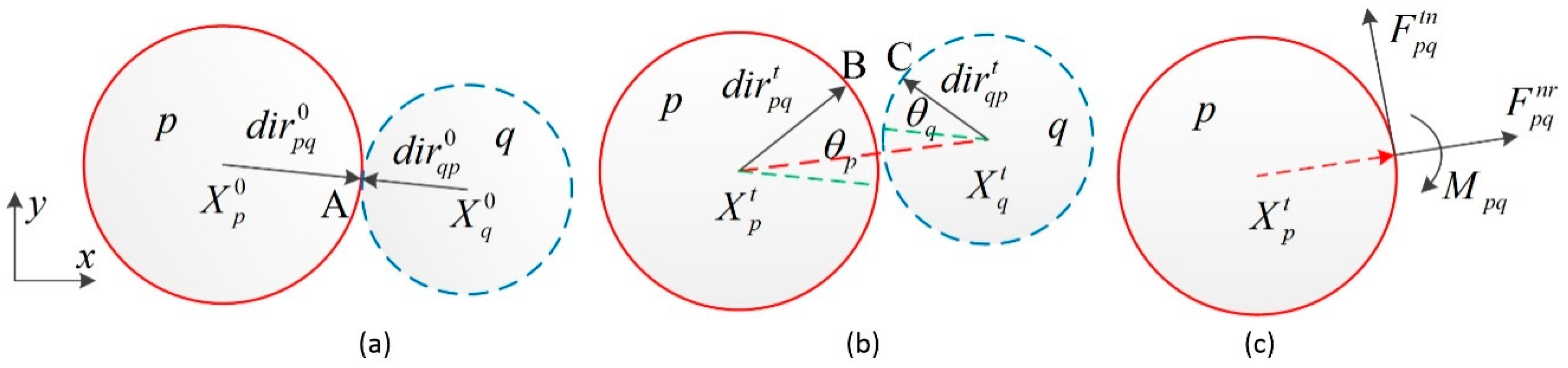
The contact particles are bonded together by the bonds, which can resist normal force, shear force and bending moment. As shown in
Figure 1a, particle
p and particle
q are in contact with each other at point A at the original states.
and
are their coordinates respectively.
and
are the vectors pointing from their centers to the contact point A respectively. At time
t, the two particles move to new positions
and
, as shown in
Figure 1b. The contact point A on particle
p move to point B and the point A on particle
q move to point C. The vector
and the vector
rotate to
and
, respectively. In addition,
and
are rotation angles of particles
p and
q in time
t respectively, defining anticlockwise as positive direction. The contact forces and moment applied to particle
p from particle
q via the bond are normal force
, shear force
and moment
, as shown in
Figure 1c.
The shear force and moment are determined by the following equations:
where
and
are shear stiffness and bending stiffness respectively,
is the original distance between
p and
q,
is shear strain of the bond between
p and
q which is the ratio of deformation in tangential direction to
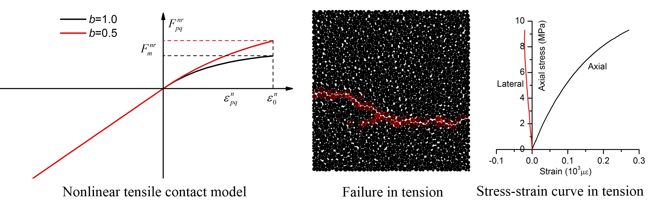
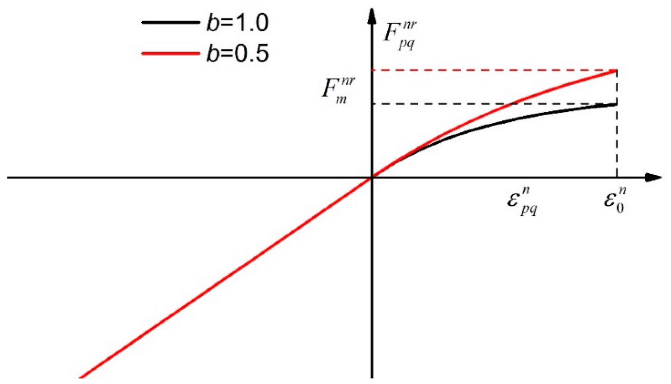
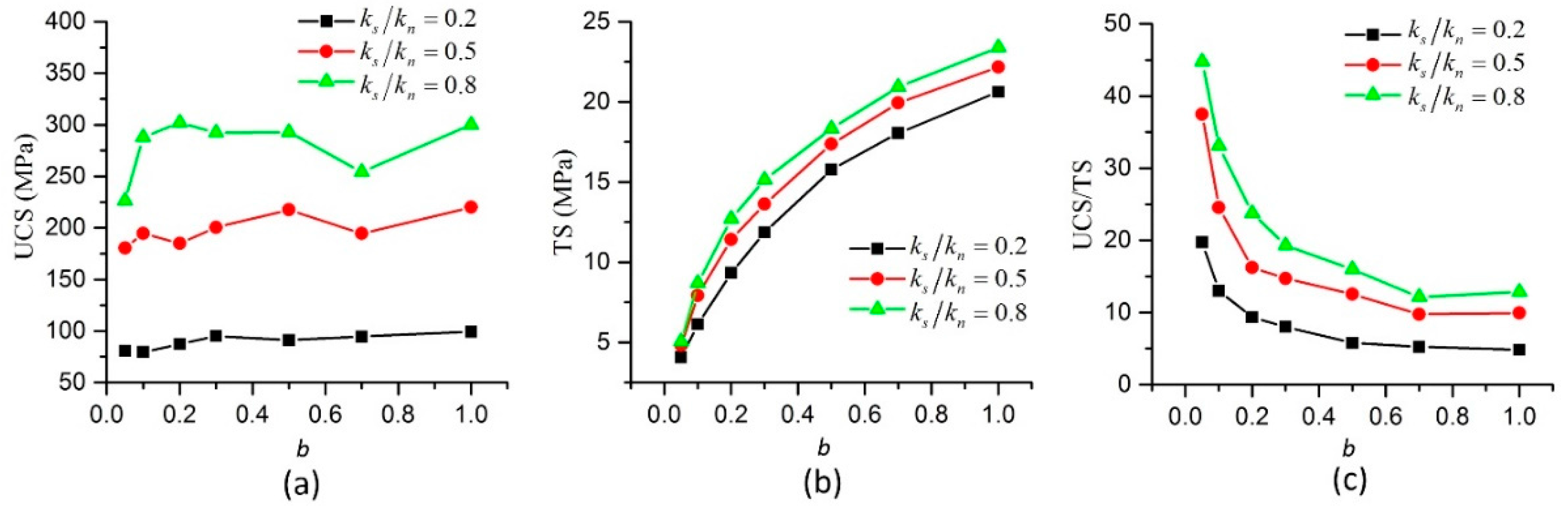
. A nonlinear elastic tensile stiffness model is proposed to describe the relationship between normal force and normal strain undergoing tension. Then the force in normal direction is expressed as:
where
is normal stiffness,
is normal strain of the bond between
p and
q, the
b is shape coefficient of the nonlinear elastic model and
is the ultimate normal tensile strain.
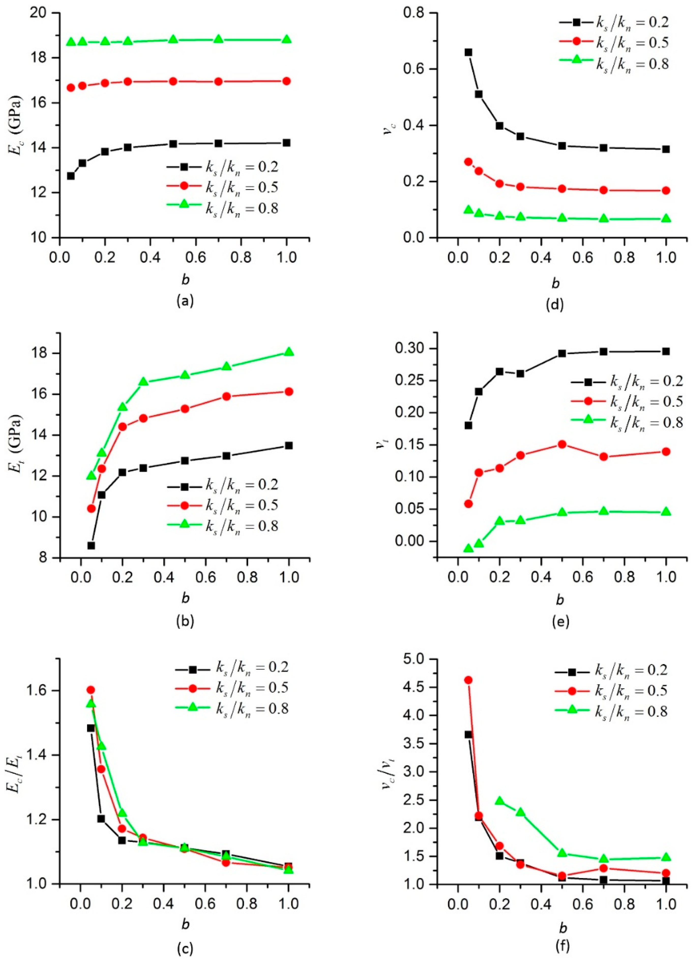
Figure 2 presents the relationship between normal force and normal strain with different value of
b. The value of
b has great effect on the normal force versus normal strain curve and the ultimate normal tensile force,
.
and
which is the increment of
in each time step are given by:
where
is the distance between the centers of
p and
q at time
t,
and
are the radii of particles
p and
q respectively,
and
are the centroid displacements of particles
p and
q respectively,
is an unit vector obtained by rotating the unit vector which points to the center of
q from the center of
p 90 degrees in the anticlockwise direction,
is time step.
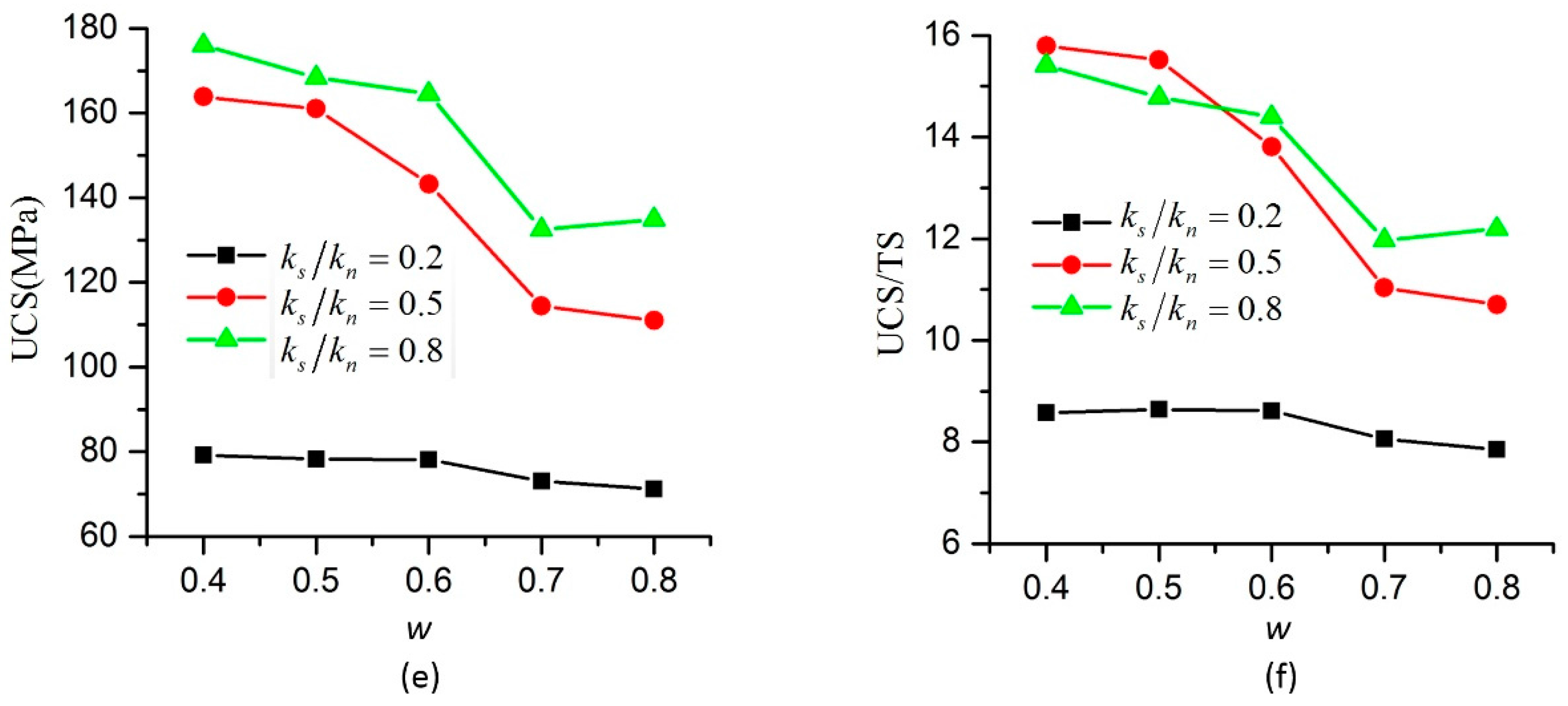
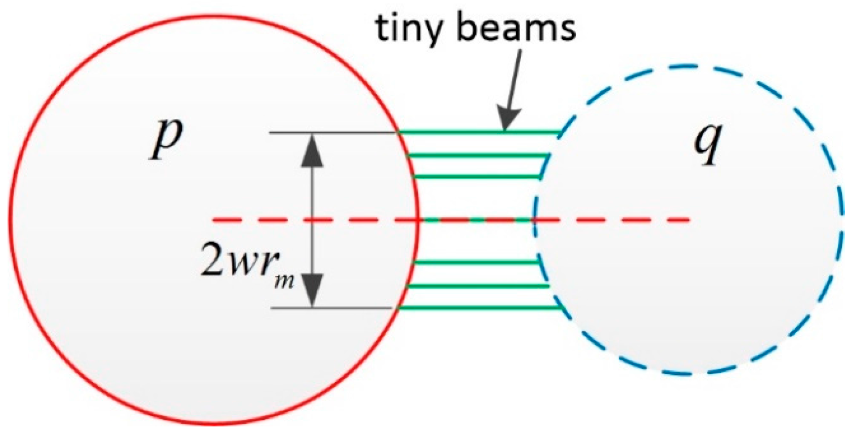
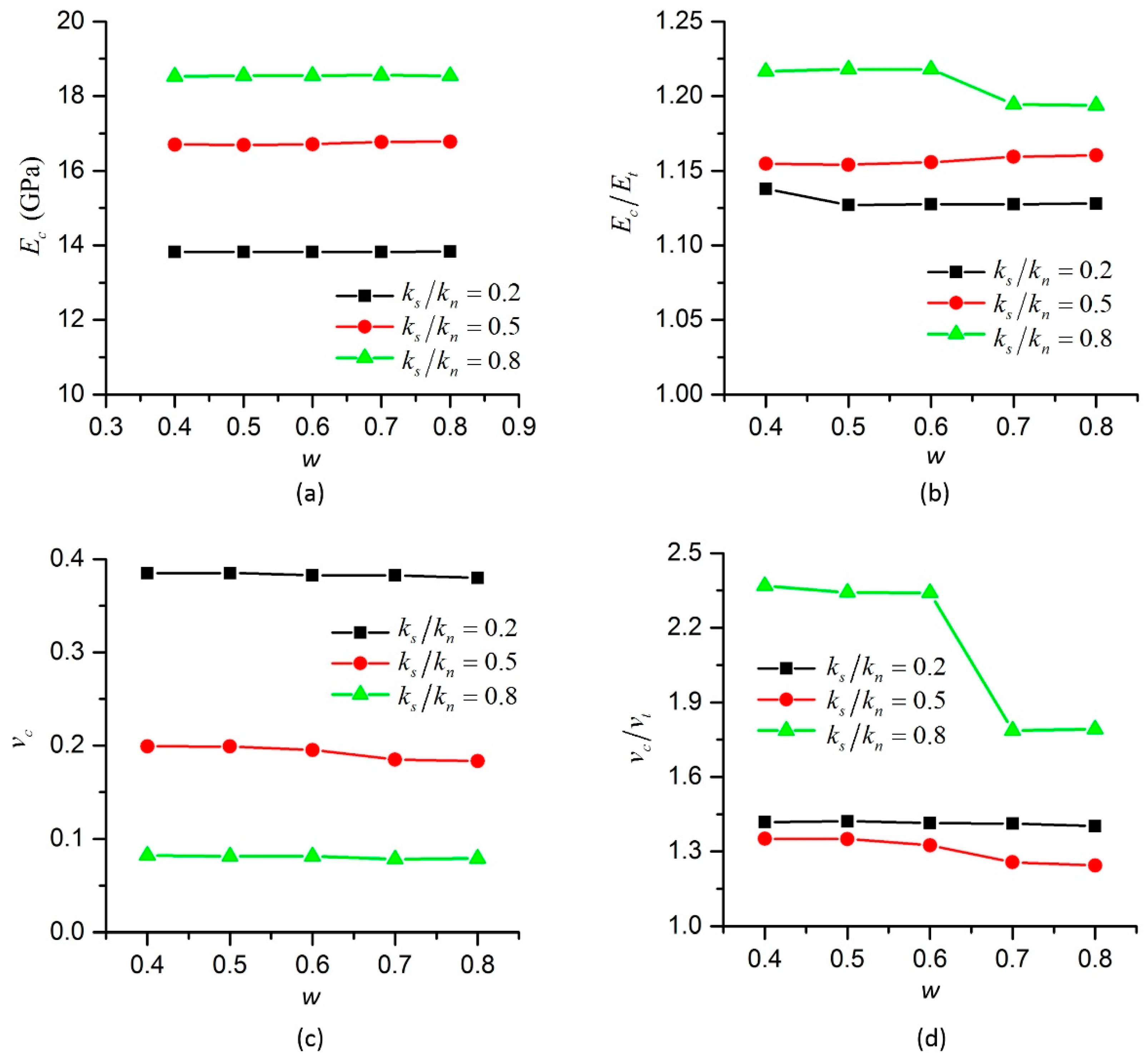
Another modification to the BPM is that the bonds are assumed as many tiny elastic beams, which distribute between two contact particles in a region wide 2
wrm and are parallel to the center line of the two particles, as presented in
Figure 3, where the
w is bond width coefficient,
rm is the smaller one of
rp and
rq. The range of
w is from 0 to 1 and that
w equals 0 means all the tiny beams gather in the center line of the two contact particles. Bonds with different bending stiffness but with the same normal stiffness and shear stiffness can be modelled by changing the distribution of the tiny beams.
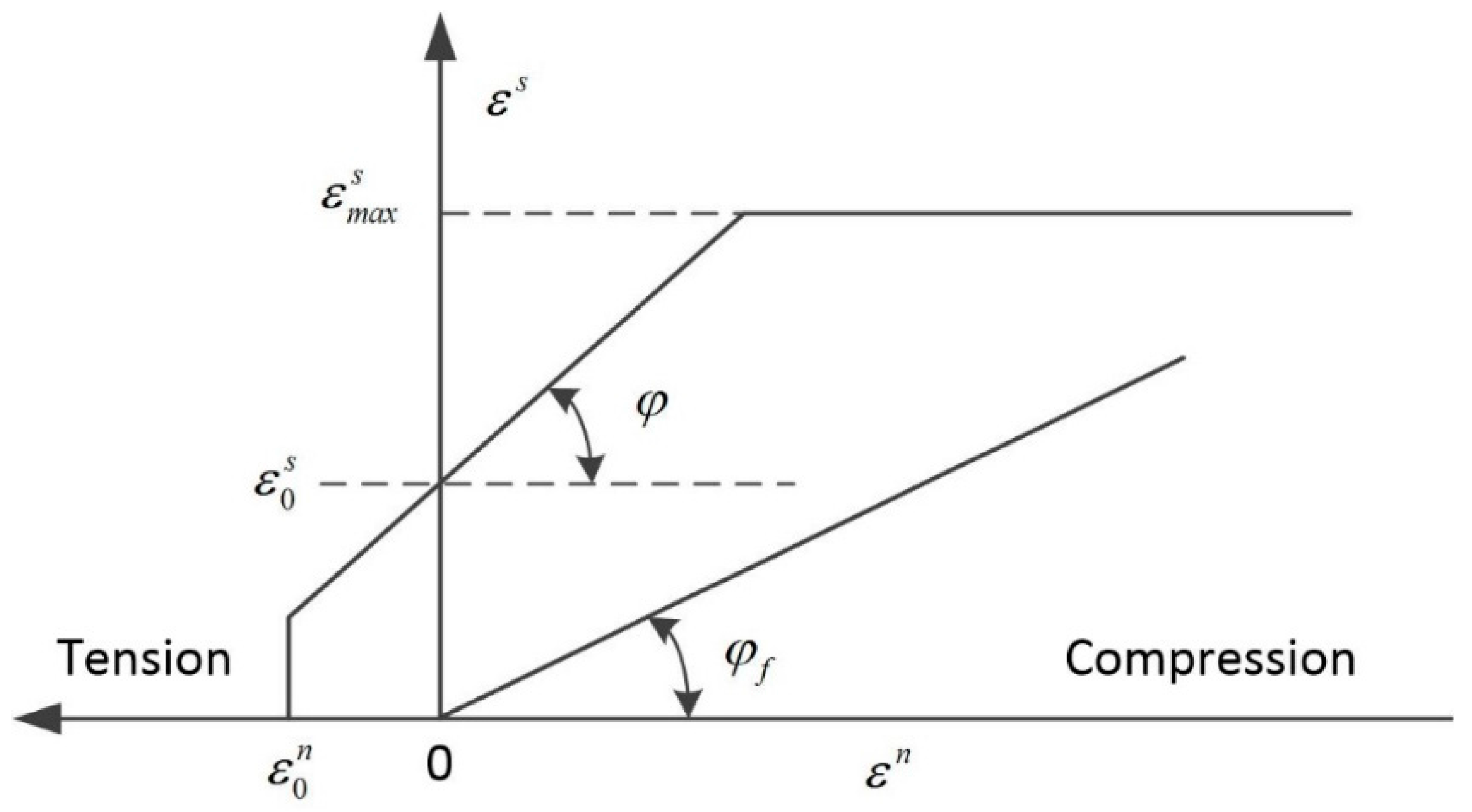
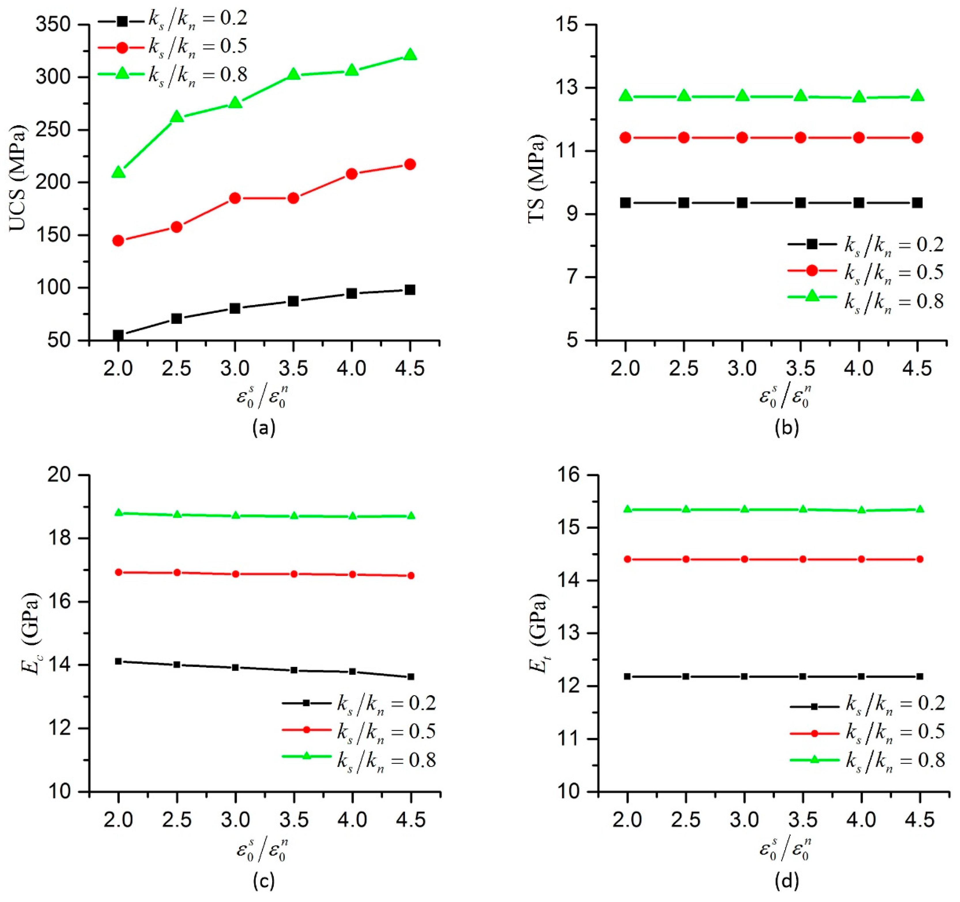
The modified Mohr-Coulomb criterion with a tension cut-off and an upper bound is used for the shear strength of the bonds, as shown in
Figure 4, where
is the upper bound of shear strain,
is the ultimate pure shear strain of the bond,
is the internal friction angle and
is the friction angle between particles when the bond between them fails. In this paper, the stresses are replaced by the strains in order to obtain better simulation results by cooperating with the nonlinear tensile model and the effect of the bend on the tensile strain is taken into consideration as follows.
If the bond is broken or no bond exists between particles
p and
q which contact with each other, then only normal force and shear force exist between them. The normal force
is calculated by Equations (3) and (4).
in Equation (4) should be replaced by the sum of the radii of
p and
q. The shear force
is calculated as follows:
where
is the coulomb friction coefficient.
The resultant contact force vector
and the resultant contact moment
on particle
p are calculated as follows:
where
is an unit vector pointing from the center of particle
p to the center of particle
q.
is a set of particles which are in contact with particle
p.
2.2. Numerical Simulation Model
The disc-shaped particles are considered as rigid bodies and their translational motions and rotational motions are governed by the standard equations of rigid body dynamics:
where
and
are the external force vector and external moment applied to particle
p respectively.
and
are mass and moment of inertia of particle
p respectively.
and
are damping force and damping moment respectively, which are introduced to dissipate kinetic energy and gain a quasi-static state of equilibrium of the particles and are expressed as [
34]:
where
and
are translational and rotational damping constant respectively. The centroid displacement and rotation angle of particle
p can be obtained by using an explicit central difference method to integrate Equations (10) and (11). The algorithm is described as follows:
where the superscript
indicates
th step.
should not exceed the critical time step
to remain numerical stability as introduced in [
34].
The forces and moments are transmitted through the contacts between particles or the contacts between particles and plates. There are two kinds of particle contacts according to whether an effective bond exists between the contact particles: the bonded particle contacts and the unbonded particle contacts. Two particles
p and
q are bonded together in the original rock specimens if their relative position satisfies the Equation (18):
where
is a nonnegative constant defined by user to eliminate the numerical errors caused during the particle generating. The errors may result in separation of two particles which should touch each other. A bond is created between every bonded particles. If
is too large, it would lead to forming bond between two particles far away from each other. In our model,
= 0.001 is suggested. When the bond is broken, the bonded particle contact becomes unbonded particle contact. Furthermore, two particles
p and
q which are not close to each other may approach each other during the simulation process, and form an unbonded particle contact when their relative position satisfies the Equation (19):
The forces and moments on the bonded particle contacts are calculated by Equations (1)–(3). While forces on the unbonded particle contacts, where no moment exists are calculated by Equations (3) and (7). The bonded particle contacts are identified at the beginning of the simulation and updated in each time steps if any bond is broken. The unbonded contacts should be identified in every time steps.
In order to improve the computational efficiency, background grids and cells are introduced in searching particle contacts. In each step, all the particles are stored in the cells formed by the grids according to their centroid position coordinates. The cell size is equal to , where is the maximum radius of the particles and is a user-defined parameter, which is positive and very small to obtain high searching efficiency. The suggested value for is 0.01 in our model. A particle can only form a particle contact with particles located in the same cell with it and with particles located in the neighbor cells. To avoid duplicate calculation, particles in cell j are only used to try to form particle contacts with particles in cell j or in neighbor cells whose numbers are larger than j.
2.3. Dimensionless Parameters in NET-BPM
In the conventional BPM, the micro parameters are normal stiffness
, shear stiffness
, bending stiffness
, ultimate normal strain
, ultimate pure shear strain
, upper bound of shear strain
, ultimate relative rotation angle
, friction angles
and
, translational damping constant
and rotational damping constant
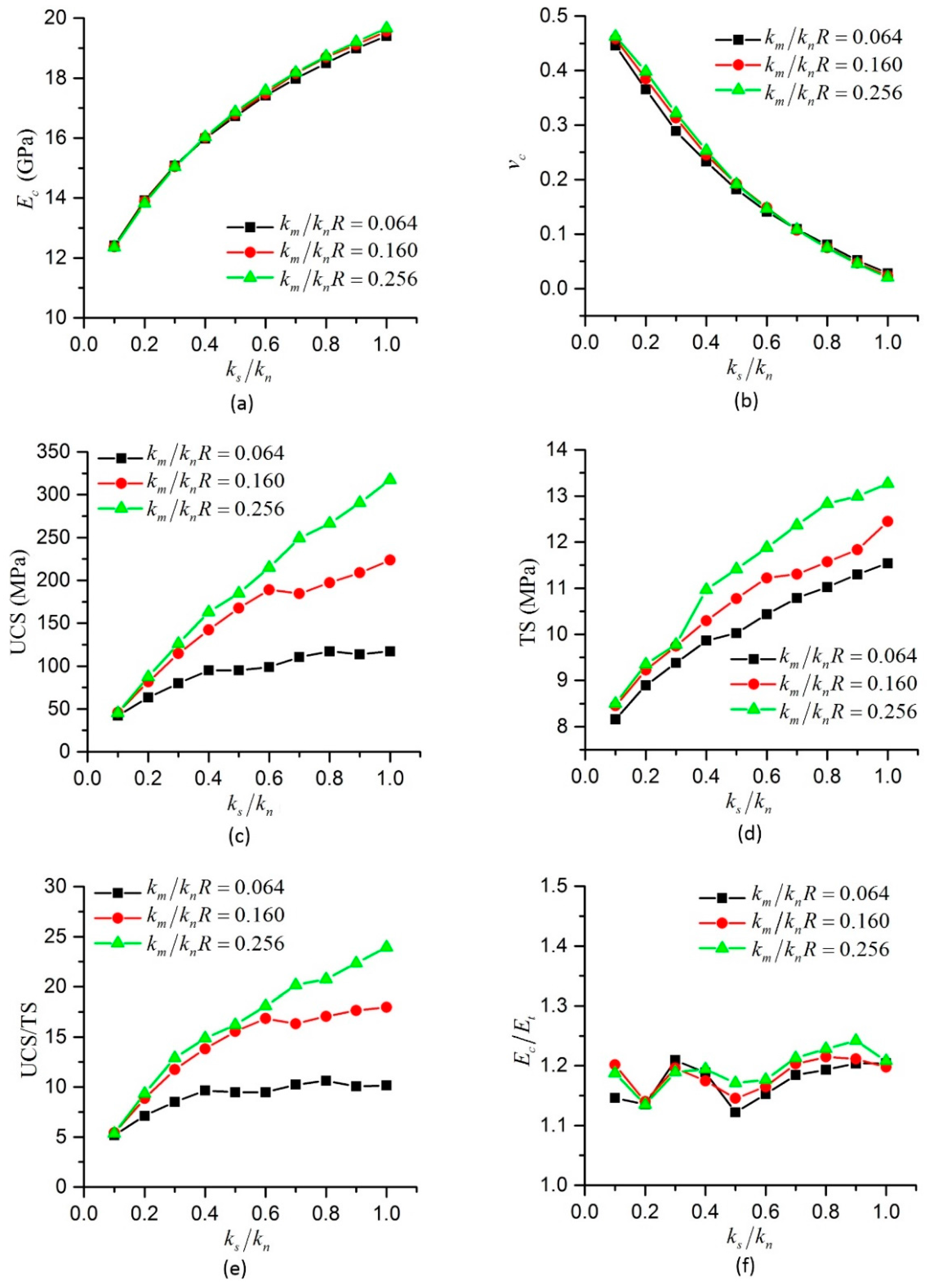
, etc. The macro parameters are UCS, TS, the ratio of UCS/TS, Young’s modulus
E and Poisson’s ratio
v, etc. A few more micro parameters, which are
w and
b are included in the NET-BPM. In addition, because Young’s modulus and Poisson’s ratio in compression and tension are different, they are denoted as
Ec and
Et,
vc and
vt, respectively. In this paper, the effects of particle size, particle arrangement, porosity and density of the specimens are not investigated. Young’s modulus and Poisson’s ratio discussed here are the apparent ones. By using dimensionless analysis similar to [
28,
34], the dimensionless micro parameters are
ks/
kn,
km/(
knR),
,
,
,
,
w,
b, and the dimensionless macro parameters are
EcR2/
kn,
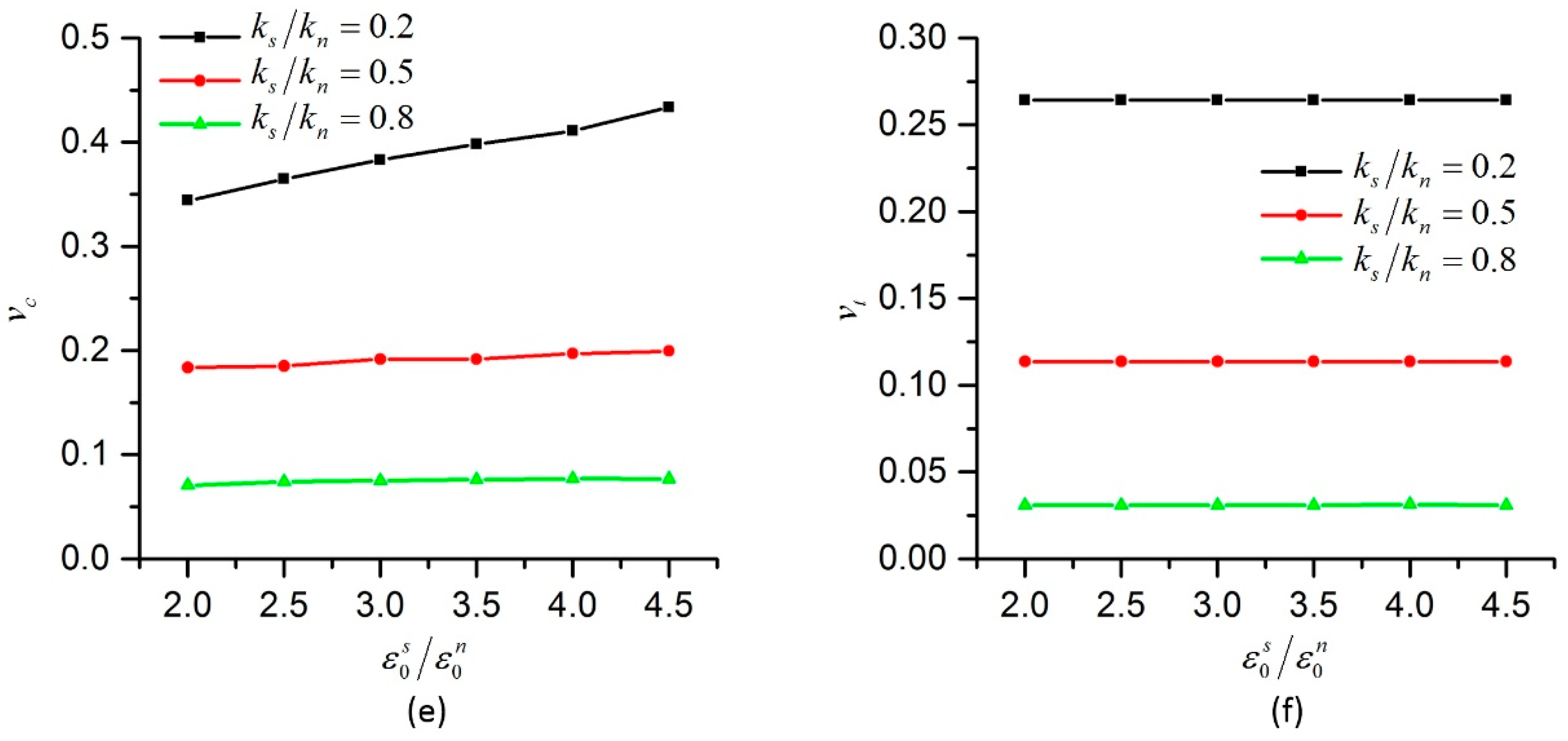
vc,
,
,
Et/
Ec,
vt/
vc in our model.
R is the characteristic length which is equal to
Rmax. As the nonlinear elastic model is applied, the ratio of
Ec to
Et and the ratio of
vc to
vt are not equal to 1 anymore, so
Et/
Ec and
vt/
vc should be taken into consideration.
2.4. Specimen Preparation
Uniaxial compression tests and direct tension tests are simulated in this study. The rock specimens used for simulations are created by the particle generating method proposed in [
44], which can create dense and stable particle packings with disks once the geometric contour of the specimen and the minimum and maximum particle size are given. The effect of the size of particles and specimens on our method is not concerned in this study. Thus, square specimens with length
L = 50 mm created by the method from [
44] with
Rmax = 0.9 mm and minimum particle radius
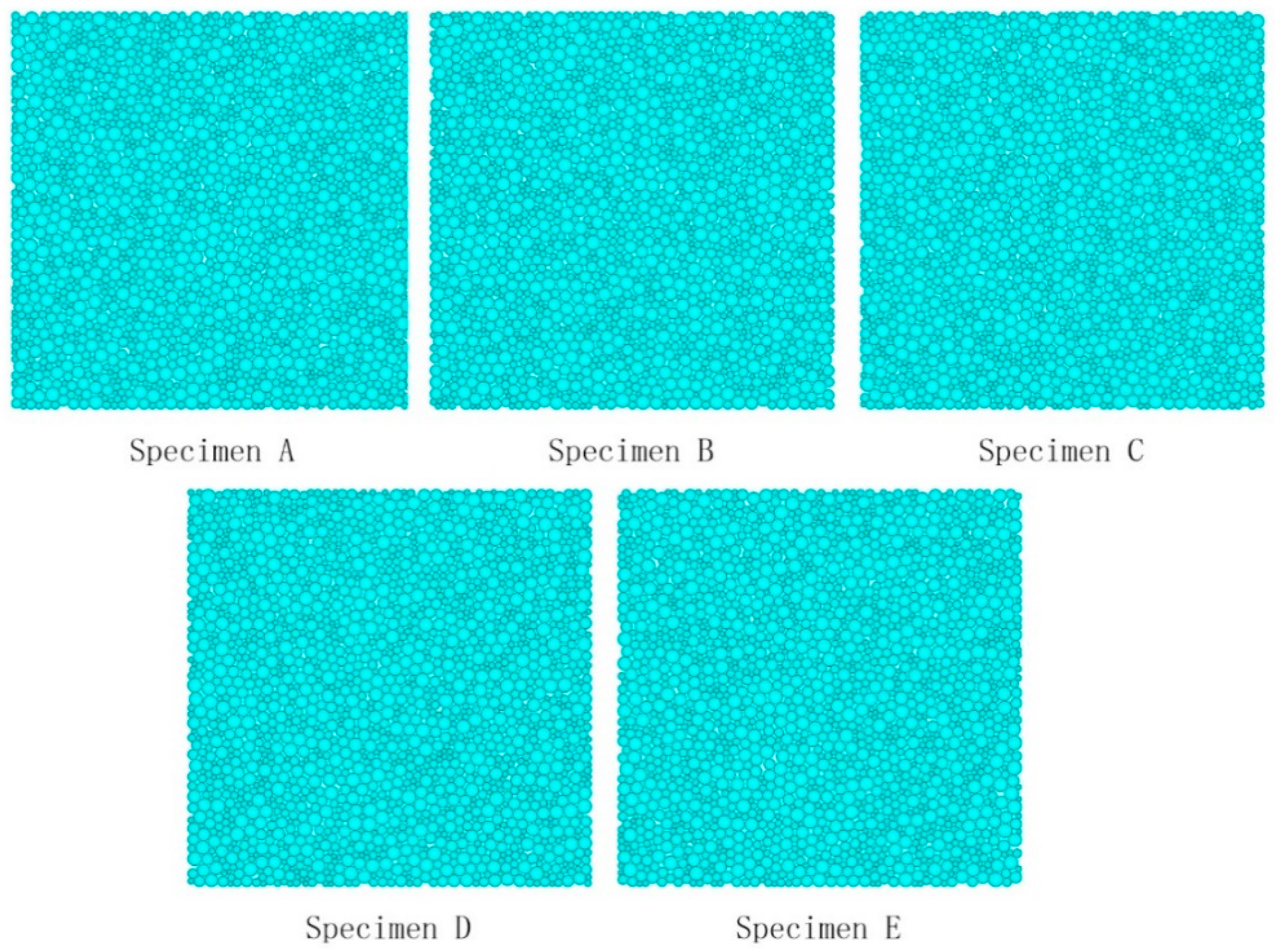
Rmin = 0.3 mm are used for our simulations. Five specimens are created by using different seeds in the initiation of the particle generation, as shown in
Figure 5. They are used to study the effects of the particle arrangement on the simulations. Some main parameters of the specimens are listed in
Table 1, where
Ra is the average radius of the particles and overlap ratio is the ratio of the overlap length to the sum of the radii of the two overlap particles.
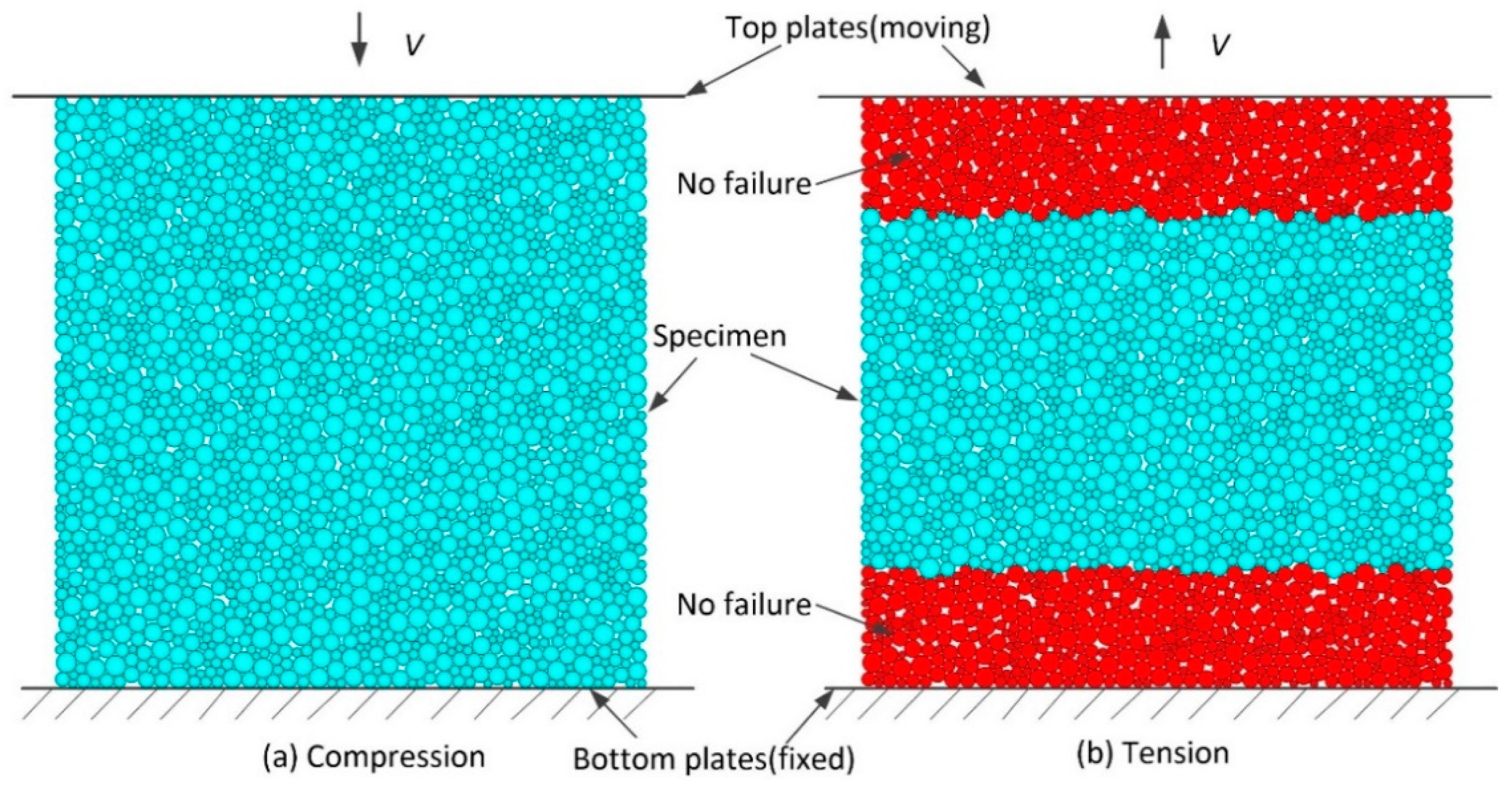
As presented in
Figure 6, when the uniaxial compression tests are simulated, the specimens are placed between two parallel plates which are considered as rigid bodies. The bottom one is fixed and the top one moves towards the bottom one with a given constant velocity,
V. When the direct tension tests are simulated, the particles in the specimens near the top and bottom boundaries are fixed to the top and bottom plates respectively and have the same velocity with the plate. In order to eliminate the effect of the boundaries on the simulation results, a layer with a height of 0.6
L in tensile direction and a width of
L perpendicular to the tensile direction is defined, which located in the center of the specimens. Only the bonds existing between the particles located in this layer are allowed to fail, similar to that in [
12]. The bottom plate is fixed and the top plate moves away from the bottom one with a constant velocity
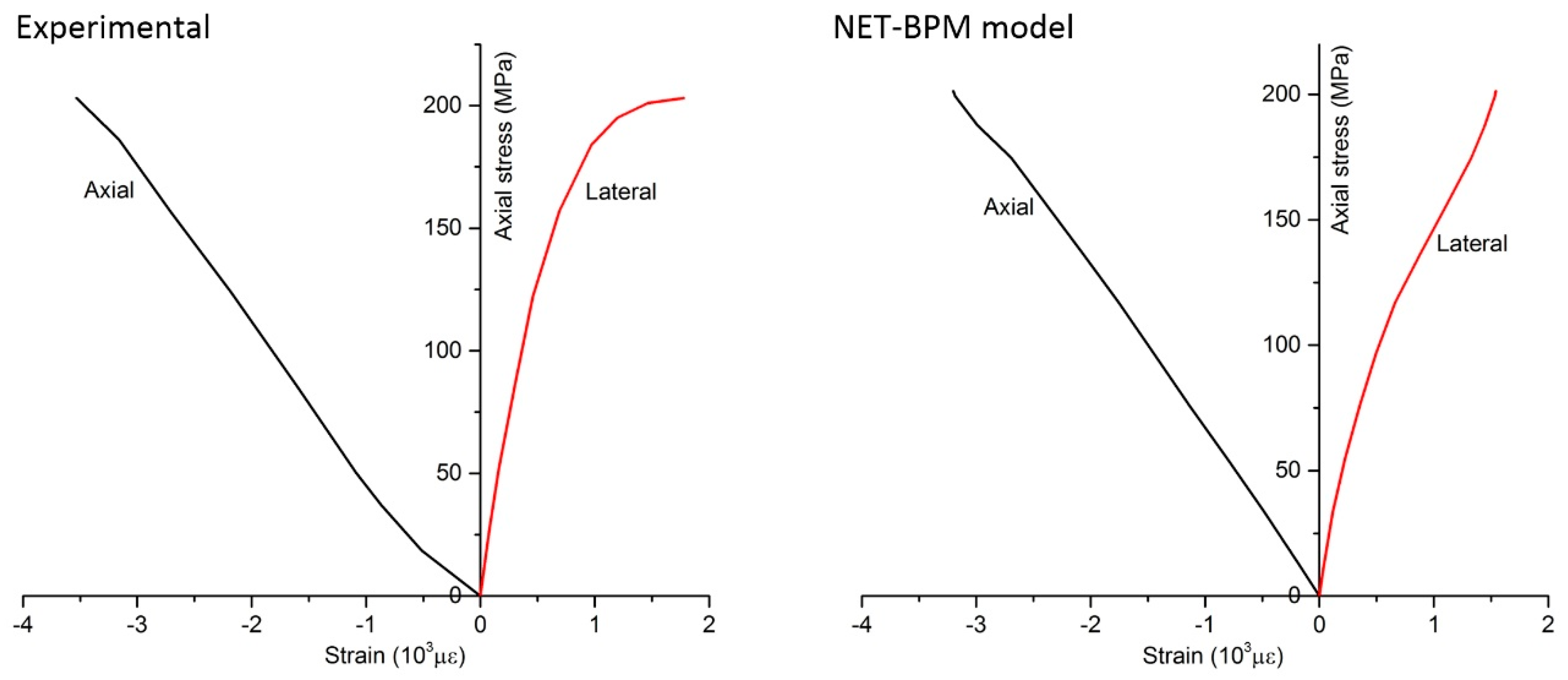
V. The lateral strain of the specimens is determined by the displacement of two particle groups. One particle group consists of four particles, which are closer to the middle point of the left side boundary of the specimen than other particles at the initial time. The other particle group consists of four particles, which are closer to the middle point of the right side boundary than other particles. The average distance of the two groups of particles in the direction perpendicular to the loading direction at the initial time and its variation during simulations are used to calculate the lateral strain. The axial strain is determined by the displacement of the two rigid plates. The loads are calculated by averaging the forces on the top and bottom plates. UCS and TS can be obtained by dividing the ultimate loads by the width of the specimen. The thickness of the specimen is assume to be 1 m in 2-D.
Ec,
Et,
vc and
vt are determined at the state when the load is equal to half the ultimate load and the secant lines are used to estimate them as introduced in [
8,
45,
46].
The NET-BPM model is compiled in Fortran 90 language for simulating uniaxial compression tests and direct tension tests. The values of the micro parameters in the model are presented in
Table 2. The density of the particles is set to be 2900 kg/m
3. The critical time step
= 2.5 × 10
−8 s is obtained with the method introduced in [
34] if the safety factor is set to 0.1. Thus, the time step
= 10
−8 s is proper in our model. The loading speed
V = 0.1 m/s in both compression and tension tests. Damping constant
and
are set to be 0.02 which are proved to be large enough to guarantee the quasi-static state of equilibrium of the particles. All five specimens presented in
Figure 5 are used for simulations with the micro parameters in
Table 2.
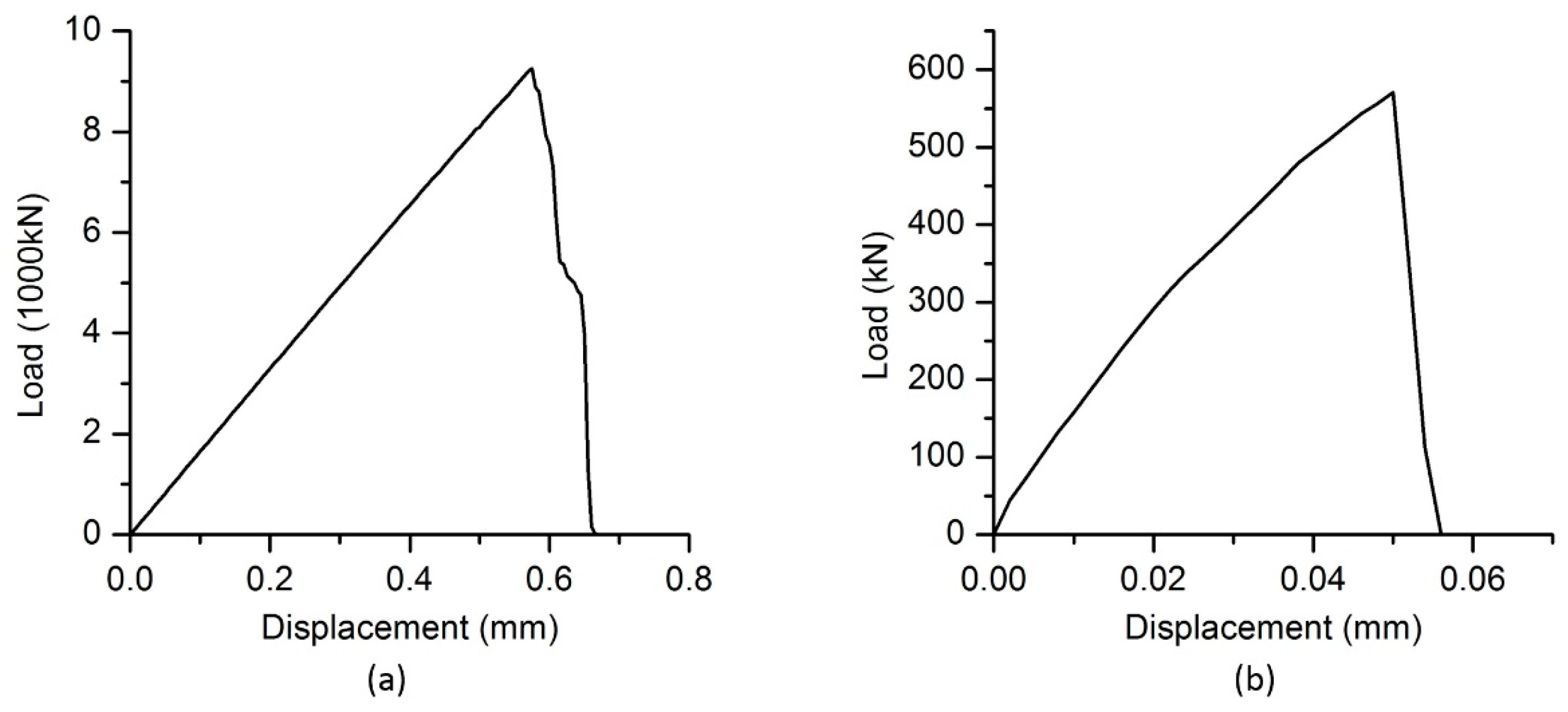
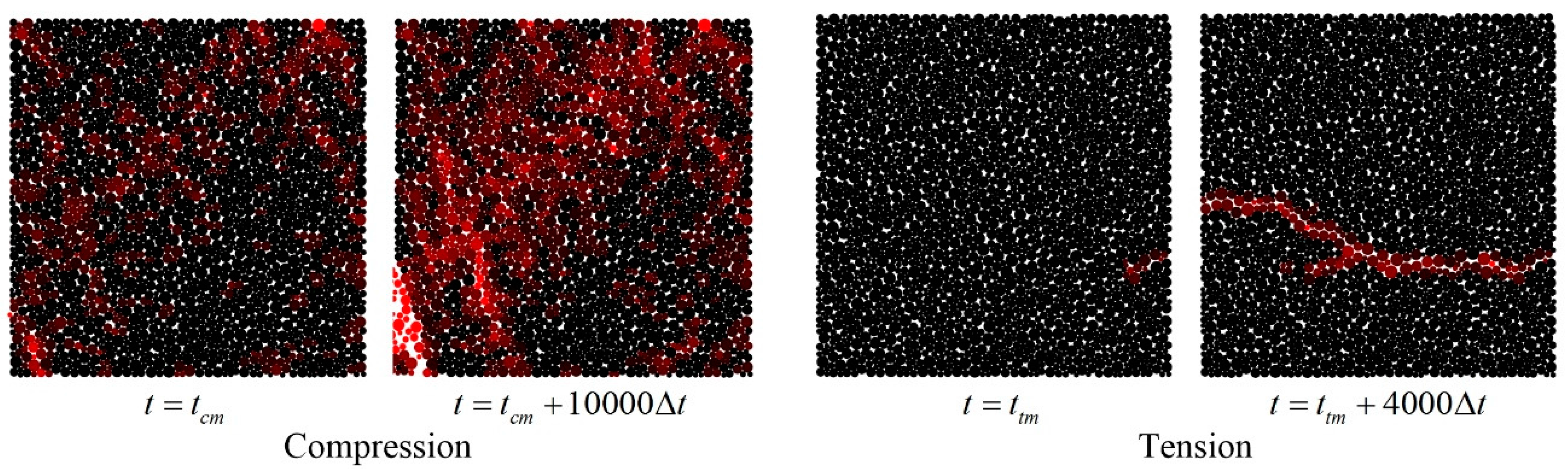
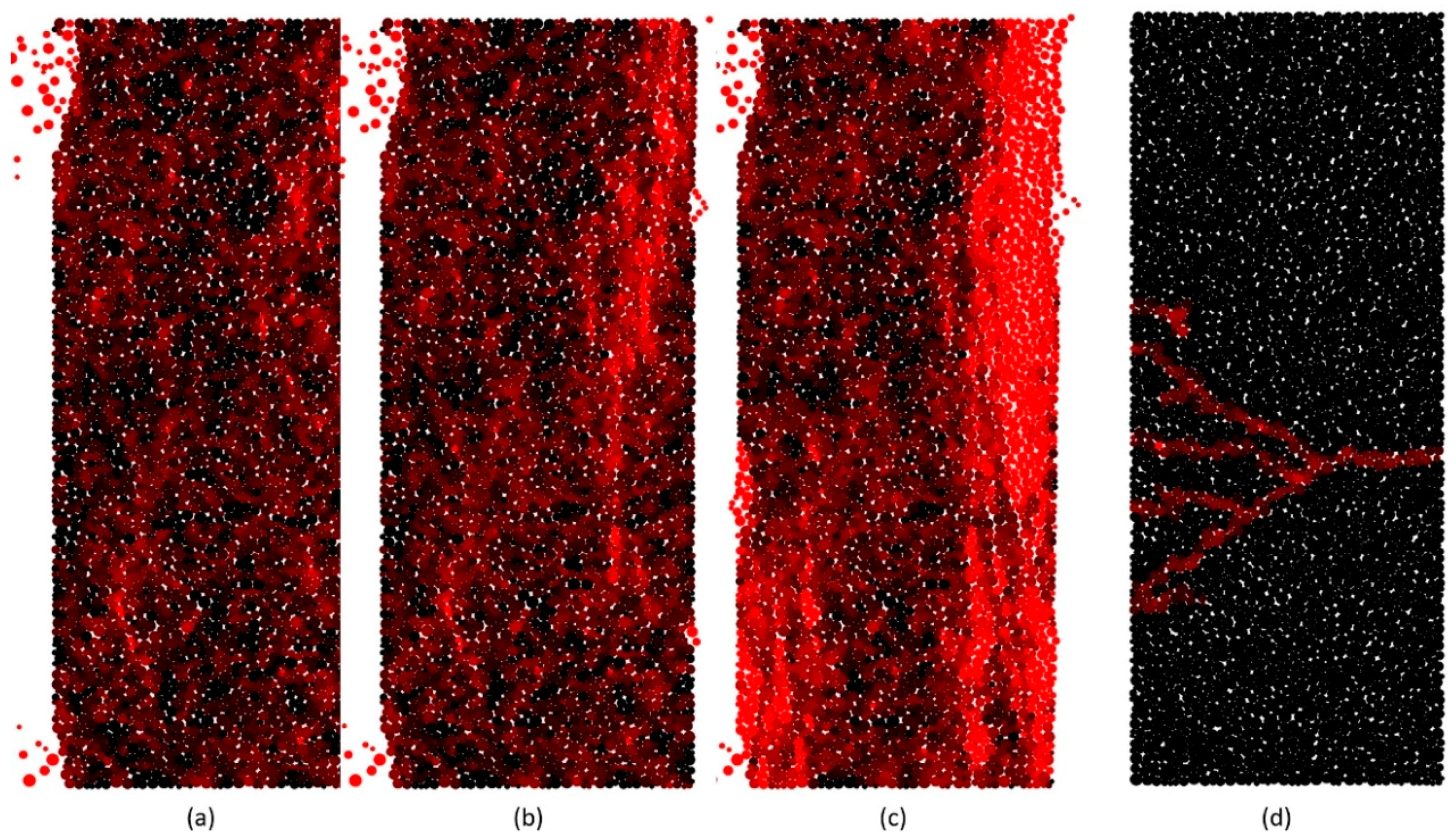
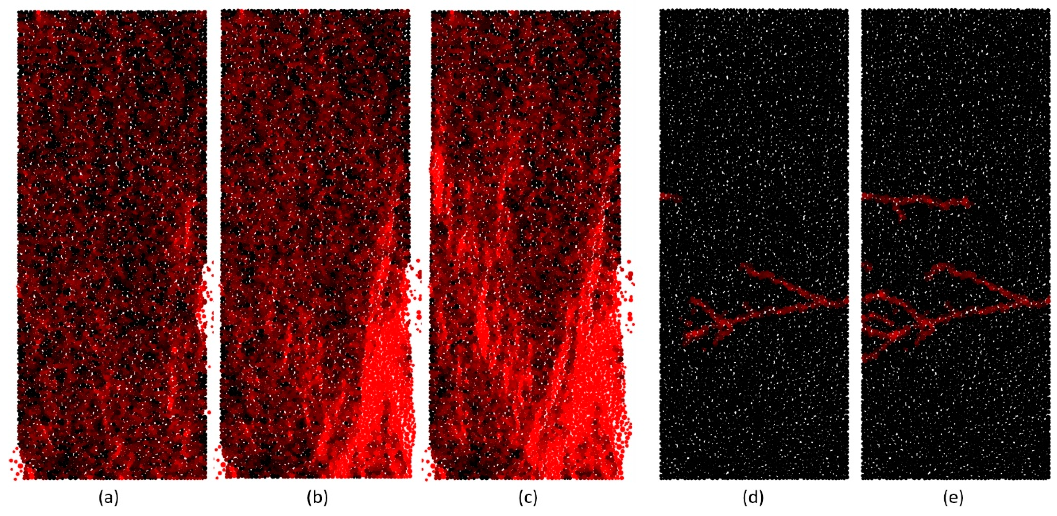
A simulation case costs about two hours on a machine with an Intel Core 5 3.2 GHz Processor. The compressive loads and tensile loads of specimen A at different displacements are presented in
Figure 7. The creak patterns of specimen A under compression and tension are shown in
Figure 8. The
tcm and
ttm are the time when the loads reach their peak values in compression and tension, respectively. The color of the particle varies from black to red gradually according to the ratio of the present number to the original number of the bonded contacts on the particle, which varies from 1 to 0. Tensile failure is the dominant failure pattern of the bonded contacts in both uniaxial compression tests and direct tension tests. The number of the failed bonded contacts was 420 by the time
t =
tcm, which increased sharply to 931 after 10,000 time steps in compression test. The number of the failed bonded contacts was 7 by the time
t =
ttm, which increased sharply to 88 after 4000 time steps in tension test. Only one main crack appeared in tension test, which is almost perpendicular to the tensile direction, but several oblique cracks appeared in compression tests. All cracks observed in our simulation are similar to those observed in experiments presented in [
47,
48].
The properties of specimen A–E from the simulations are listed in
Table 3. It shows that the difference of the properties between different specimens is small. The maximum ratio of the stand deviation value to the average value is 0.15. This indicates that the specimens created by the method in [
44] with the same
Rmax and
Rmin share almost the same properties.


