A Free Interface Model for Static/Flowing Dynamics in Thin-Layer Flows of Granular Materials with Yield: Simple Shear Simulations and Comparison with Experiments

Abstract

Flows of dense granular materials comprise regions where the material is flowing, and regions where it is static. Describing the dynamics of the interface between these two regions is a key issue to understanding the erosion and deposition processes in natural environments. A free interface simplified model for non-averaged thin-layer flows of granular materials has been previously proposed by the authors. It is a coordinate-decoupled (separated variables) version of a model derived by asymptotic expansion from an incompressible viscoplastic model with Drucker-Prager yield stress. The free interface model describes the evolution of the velocity profile as well as the position of the transition between static and flowing material. It is formulated using the coordinate Z in the direction normal to the topography and contains a source term that represents the opposite of the net force acting on the flow, including gravity, pressure gradient, and internal friction. In this paper we introduce two numerical methods to deal with the particular formulation of this model with a free interface. They are used to evaluate the respective role of yield and viscosity for the case of a constant source term, which corresponds to simple shear viscoplastic flows. Both the analytical solution of the inviscid model and the numerical solution of the viscous model (with a constant viscosity or the variable viscosity of the $\mu (I)$ rheology) are compared with experimental data. Although the model does not describe variations in the flow direction, it reproduces the essential features of granular flow experiments over an inclined static layer of grains, including the stopping time and the erosion of the initial static bed, which is shown to be closely related to the viscosity for the simple shear case.

1. Introduction

Understanding and theoretically describing the static/flowing transition in dense granular flows is a central issue in research on granular materials, with strong implications for industry and geophysics, in particular in the study of natural gravity-driven flows. Such flows (e.g., landslides or debris avalanches) play a key role in erosion processes on the Earth’s surface and represent major natural hazards. In recent years, significant progress in the mathematical, physical, and numerical modeling of gravity-driven flows has made it possible to develop and use numerical models for the investigation of geomorphological processes and assess risks related to such natural hazards. However, severe limitations prevent us from fully understanding the processes acting in natural flows and predicting landslide dynamics and deposition, see e.g., [1]. In particular, a major challenge is to accurately describe complex natural phenomena such as the static/flowing transition.

Geophysical, geotechnical, and physical studies have shown that the static/flowing transition related to the existence of no-flow and flow zones within the mass plays a crucial role in most granular flows and provides a key to understanding their dynamics in a natural context, see [1] for a review. This transition occurs in erosion-deposition processes when a layer of particles flows over a static layer or near the destabilization and stopping phases. Note that natural flows often travel over deposits of past events, which may or may not be made of the same grains, and entrain material from the initially static bed. Even though erosion processes are very difficult to measure in the field, e.g., [2,3,4], entrainment of underlying material is known to significantly change the flow dynamics and deposition, e.g., [5,6,7,8,9,10].

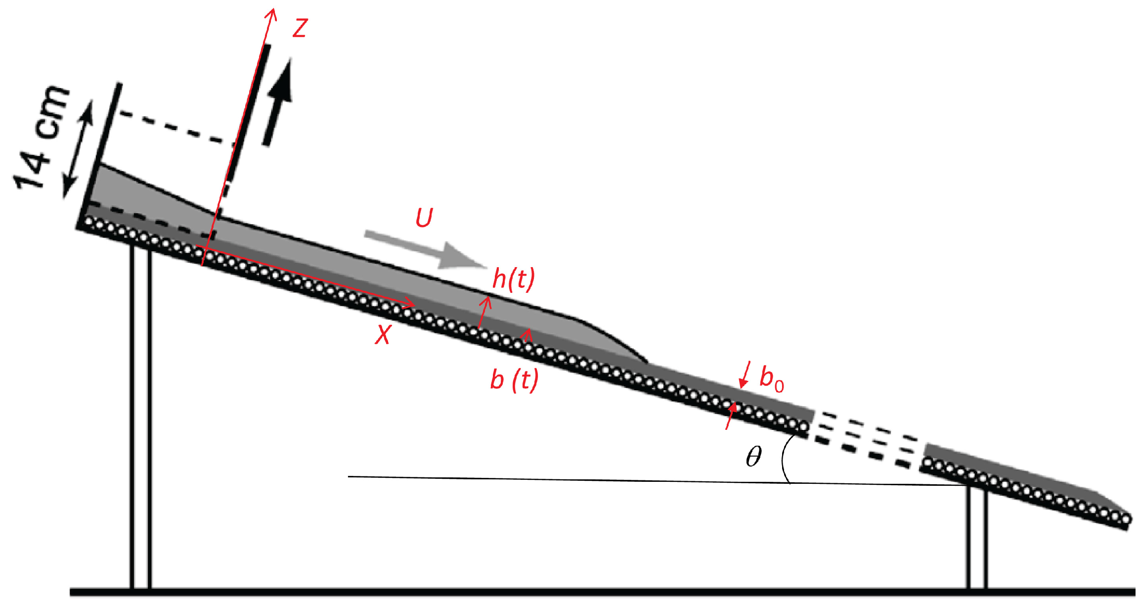
Experimental studies have provided some information on the static/flowing dynamics in granular flows, showing for example that the presence of a very thin layer of erodible material lying on an inclined bed may increase the maximum runout distance of a granular avalanche flowing down the slope by up to $40\%$ and change the flow regimes [9,11,12]. 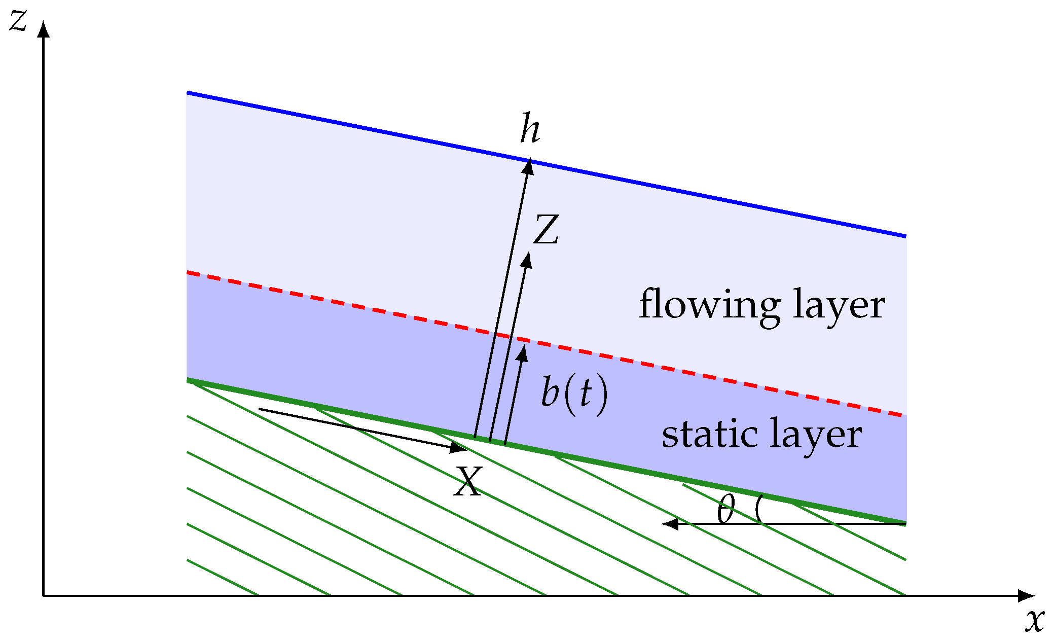In these experiments that mimic natural flows over initially static beds (Figure 1), quasi-uniform flows develop when the slope angle $\theta$ is a few degrees lower than the typical friction angle $\delta$ of the involved material [12]. 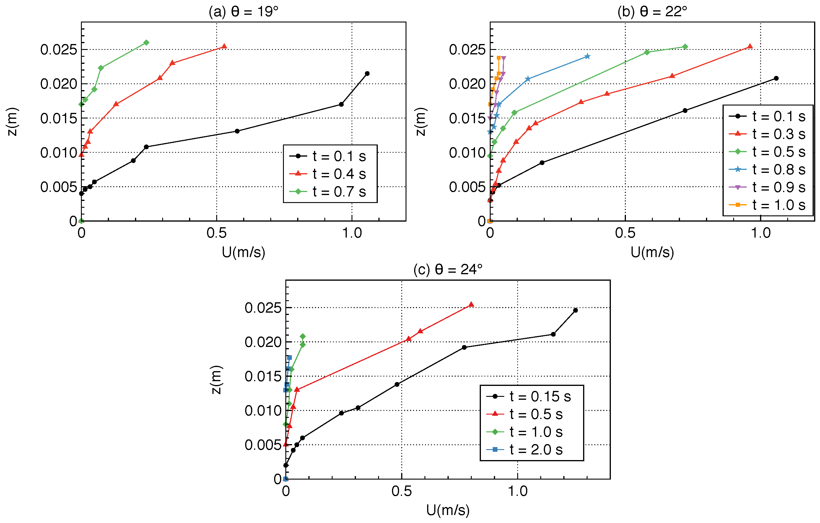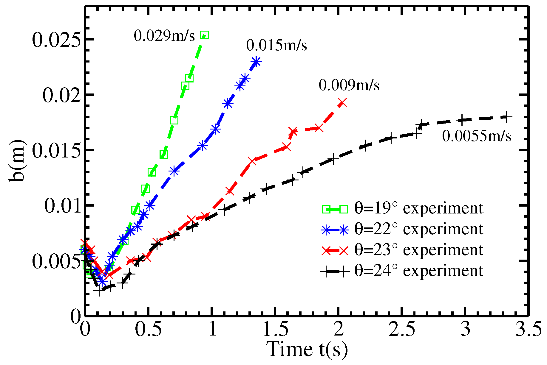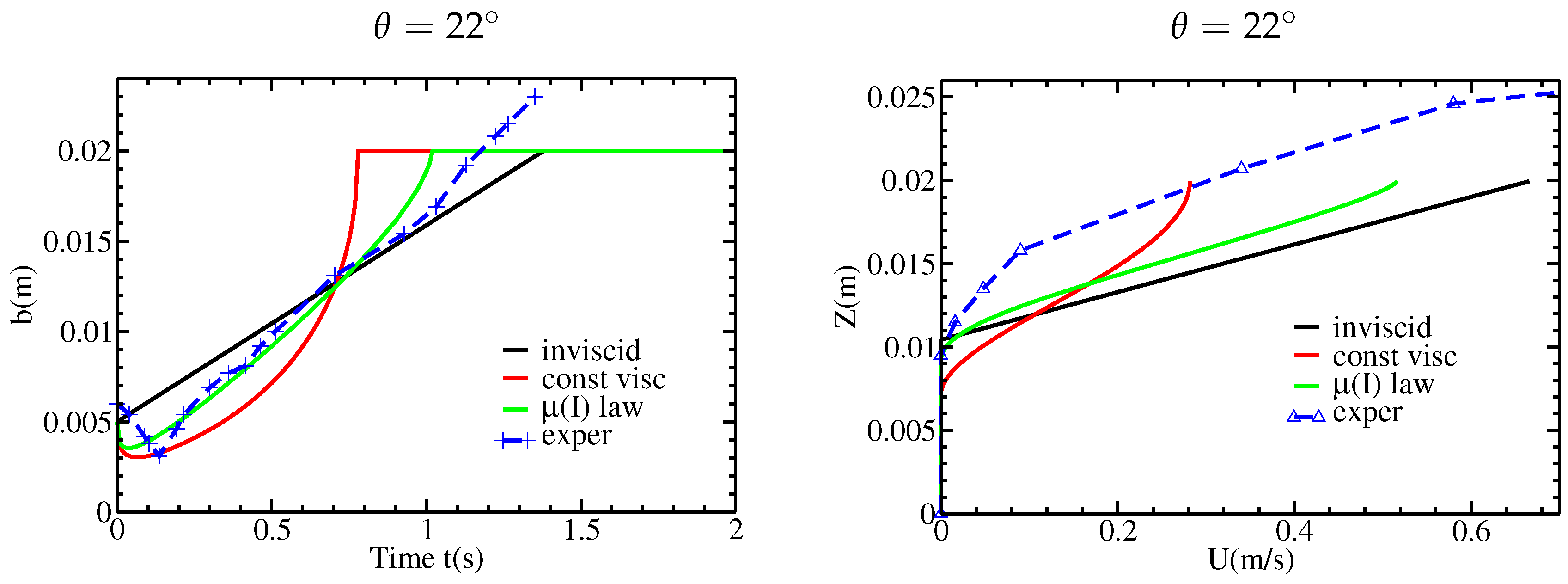Figure 2 and Figure 3 show new data extracted from the experiments performed by [12] on the change with time of the static/flowing interface position b and the velocity profiles $U(Z)$ within the granular mass, where Z is the direction normal to the bed. At a given position X along the plane, the flow is shown to excavate the initially static layer immediately when the front reaches this position. The static/flowing interface rapidly penetrates into the static layer, reaching a lowest position (that depends on the slope angle) for significantly high slopes and then rises almost linearly or exponentially toward the free surface until the whole mass of material stops (Figure 2). A theoretical description of these observations is still lacking. In particular, questions remain as to what controls the change with time of the static/flowing interface position and the velocity profiles and how these characteristics are related to the rheology of the granular material and the initial and boundary conditions.

In order to alleviate the high computational costs required to describe the real topography and the rheology, which both play a key role in natural flow dynamics, thin-layer (i.e., the thickness of the flow is assumed to be small compared to its down-slope extension) depth-averaged models are generally used to simulate landslides [14]. Such models have been rigorously derived for arbitrary topography, but the static/flowing transition has generally been neglected, e.g., [15,16,17,18]. Several attempts have been made to describe this transition in thin-layer (i.e., shallow) models, in particular by deriving an equation for the static/flowing interface position or by establishing erosion/deposition rates, e.g., [19,20]. However, these approaches are generally based on debatable phenomenological laws and/or are too schematic to be extended to natural flows [21]. The simplifications used in some previous models lead to an inconsistent energy Equation [22]. Indeed, some of these models prescribe a given velocity profile to deduce the entrainment rate (see e.g., [23] or references in [22]). However, in transient flows, the velocity profile changes with time as shown for example in the multilayer shallow model of [24]. A better understanding of the non-averaged case is necessary before defining more physically relevant depth-averaged models including the static/flowing transition. This is why we focus here on non-averaged thin-layer models.

Recent work has shown that viscoplastic flow laws with yield stress describe well granular flows and deposits in different regimes, from steady uniform flows [25,26,27,28] to transient granular collapse over rigid or erodible horizontal beds [29,30,31] and inclined beds [24,32,33] or accelerating/decelerating channel flows [34]. Very good agreement with experiments is obtained even though these laws, and in particular the so-called $\mu (I)$ rheology, where I is the inertial number [28], have been shown to be ill-posed in the quasi-static regime, i.e., for small I (and also for large I) [35]. These promising results may be related to the use of a coarse mesh, whereby simulations avoid the ill-posedness by damping the fast-growing high wavenumbers [33]. In any case, the quasi-static regime near the static/flowing interface is known to be very complex, involving strong and weak force chains and local rearrangement of particles, e.g., [36,37] and has been widely studied, in particular using discrete element methods, e.g., [1,38,39]. This regime is not accurately described by the proposed viscoplastic laws involving a simple yield stress. Questions however remain as to whether such ‘simple’ viscoplastic laws are able to describe quantitatively the change with time of the static/flowing interface position and the velocity profiles observed experimentally for flows over an initially static bed and how the viscosity affects these processes.

Based on such a viscoplastic model with yield stress, an analytic expansion in the non-averaged thin-layer regime is provided in [40], giving a theoretical basis for equations describing the static/flowing interface dynamics in a dry granular material. A key point in this approach that fundamentally differs from previous thin-layer models (see [21] for a review) is that even if the flow is assumed to be thin, the normal coordinate Z is still present (there is no depth-averaging). The static/flowing interface is free in this approach, in the sense that it has no explicit equation defining its evolution. Its time variation is instead implicitly determined by an extra boundary condition on the velocity at this interface. The model from [40] being still too complicated, however a formal decoupling of the coordinates X in the down-slope direction and Z normal to the topography is proposed in [41], leading to a model with only the coordinate Z, but including a source term S that represents the opposite of the net force acting on the flow, including gravity, pressure gradient, and internal friction. We propose here to evaluate the dynamics produced by the free interface model of [41], for the most simple case involving a constant source S. This corresponds to assuming no dependency on the down-slope coordinate X in the model of [40]. It is also equivalent to considering simple shear solutions to the original viscoplastic model, which shows that in this case the model is valid without a smallness assumption. Although the down-slope coordinate X plays a key role in real flows, taking into account the fluctuations of the free surface, topography, and inflow information, we must first understand the dynamics when X is not involved. We show that the analysis of this simple shear system provides new insight into the change of the static/flowing interface position and the velocity profiles with time.

Because the boundary conditions and interface evolution are formulated in an uncommon way, specific methods must be used to deal numerically with the free interface model. We introduce two numerical methods that give similar grid-independent results, thereby showing that our model is well-posed for the case considered here involving only Z dependency.

The paper is organized as follows. The model of [40,41] for the case of a constant source (corresponding to simple shear flows of the viscoplastic model) is recalled in Section 2. Then, in Section 3, we derive an analytical solution for the inviscid model with a constant source term, which partly reproduces the experimental observations and shows explicitly how the static/flowing interface position and the velocity profiles are related to the flow characteristics and to the initial and boundary conditions. In Section 4, we introduce two new numerical methods for the simulation of the viscous model, with a constant viscosity or the variable viscosity associated with the $\mu (I)$ rheology. The numerical results show that, as opposed to the inviscid model, viscosity makes it possible to reproduce the initial penetration of the static/flowing interface within the static bed and the exponential shape of the velocity profiles near this interface. Finally, in Section 5, these results are discussed based on comparison with former experimental and numerical studies on granular flows, showing the key features and the limits of the non-averaged thin-layer model for providing a better understanding and modeling of laboratory and natural flows.

2. The Free Interface Model

2.1. Origin of the Model: Viscoplastic Rheology with Yield Stress

The initial governing equations express the dynamics of an incompressible ($\nabla ·\mathbf{U}=0$) viscoplastic material with Drucker–Prager yield stress,

$${\partial }_t\mathbf{U}+\mathbf{U}·\nabla \mathbf{U}-\nabla ·\sigma =-\mathbf{g},$$

(1)

with the rheological law

$$\sigma =-p\mathrm{I}d+2\nu D\mathbf{U}+{\mu }_{s}p\frac{D\mathbf{U}}{\parallel D\mathbf{U}\parallel },$$

(2)

where $\mathbf{U}$ is the velocity, $-\mathbf{g}$ gravitational acceleration, $\sigma$ the stress tensor (normalized by the density), p the scalar pressure (also normalized by the density), and $D\mathbf{U}$ the strain rate tensor $D\mathbf{U}=(\nabla \mathbf{U}+{(\nabla \mathbf{U})}^t)/2$. Here the norm of a matrix $A=(A_{ij})$ is $\parallel A\parallel ={(\frac{1}{2}{\sum }_{ij}{A}_{ij}^2)}^{1/2}$. The coefficients ${\mu }_s>0$ and $\nu \ge 0$ are the internal friction and the kinematic viscosity, respectively. In general $\nu$ and ${\mu }_s$ could depend on $\parallel D\mathbf{U}\parallel$ and p, but we shall consider ${\mu }_s$ constant here since the so-called $\mu (I)$ law can be written in this form for some viscosity $\nu$, see Section 4.5.

2.2. Free Interface Model with Source Term

A non-averaged thin-layer model for flows described by Equations (1) and (2) with a static/flowing interface has been derived in [40]. It is formulated for the coordinates X in the direction tangent to the topography and Z normal to the topography. The topography is described by its angle $\theta (X)$ with respect to the horizontal (see Figure 4 for a flat topography). For the case of simple shear (no dependency on X), no smallness assumption is necessary ([40] Section 2.3) and the model can be written as the following free interface problem with a source term. The unknowns are $U(t,Z)$ (velocity in the direction tangent to the topography) defined for $b(t)<Z<h$, where $h>0$ is the given constant thickness of the layer and $b(t)$ the unknown position of the static/flowing interface, $0<b(t)<h$. They obey the following equations,

$${\partial }_{t}U(t,Z)+S(t,Z)-{\partial }_Z\left(\nu {\partial }_{Z}U(t,Z)\right)=0\mathrm{for}\mathrm{all}Z\in (b(t),h),$$

(3)

with the following boundary conditions for all $t>0$,

$$\begin{array}{cc}\hfill U=0& \mathrm{at}Z=b(t),\hfill \end{array}$$

(4a)

$$\begin{array}{cc}\hfill \nu {\partial }_{Z}U=0& \mathrm{at}Z=b(t),\hfill \end{array}$$

(4b)

$$\begin{array}{cc}\hfill \nu {\partial }_{Z}U=0& \mathrm{at}Z=h.\hfill \end{array}$$

(4c)

The source $S(t,Z)$ is assumed to be given and represents the opposite of the net force, excluding the viscous force (see [41] and (10) below). The viscosity $\nu$ can a priori depend on t and Z in the model. The velocity is extended by defining $U(t,Z)=0$ for $0\le Z\le b(t)$, corresponding to the static domain. The initial condition is formulated as

$$U(0,Z)=U^0(Z)\mathrm{for}\mathrm{all}Z\in [0,h],$$

(5)

where $U(0,Z)$ is the limit of $U(t,Z)$ as $t\downarrow 0$. The initial velocity $U^0(Z)$ is given for $Z\in [0,h]$, such that for some $b^0\in (0,h)$ (initial position of the interface), the function $U^0$ satisfies $U^0(Z)=0$ for $Z\in [0,b^0]$, and ${\partial }_Z{U}^0>0$ for $Z\in (b^0,h)$. The system is completed by the static equilibrium condition

$$S(t,b(t))\ge 0\mathrm{for}\mathrm{all}t\in (0,T],$$

(6)

that states that the net force must be resistive in the static layer. The velocity U obtained when solving (3)–(6) is expected to satisfy ${\partial }_{Z}U>0$ for $b(t)<Z<h$. As proved in [41], this is the case as soon as ${\partial }_{Z}S\le 0$ and $\nu >0$.

The unusual nature of the system (3)–(6) lies in the fact that the interface position $b(t)$ is free, meaning that it has no given equation relating $\dot{b}(t)\equiv db/dt$ to other quantities. Its evolution is instead implicitly governed by the boundary conditions (4a) and (4b). An interesting property of the model (3)–(6) is that a differential equation can nevertheless be derived for the time evolution of the position of the interface, valid under some conditions, as follows (see [41]).

• If $\nu >0$ then

  $${\partial }_Z\left(\nu {\partial }_{Z}U\right)(t,b(t))=\nu {\partial }_{ZZ}^{2}U(t,b(t))=S(t,b(t)),$$

  (7)

  and whenever $S(t,b(t))\ne 0$, one has

  $$\dot{b}(t)=\left({\displaystyle \frac{{\partial }_{Z}S(t,b(t))-{\partial }_{ZZ}^2(\nu {\partial }_{Z}U)(t,b(t))}{S(t,b(t))}}\right)\nu .$$

  (8)
• If $\nu =0$ and ${\partial }_{Z}U(t,b(t))\ne 0$, then

  $$\dot{b}(t)={\displaystyle \frac{S(t,b(t))}{{\partial }_{Z}U(t,b(t))}}.$$

  (9)

These formulas show the strong interrelationship between the velocity profile in the direction perpendicular to the inclined plane and the evolution of the static/flowing interface position. Erosion, i.e., penetration of the static/flowing interface into the erodible bed, occurs when $\dot{b}(t)<0$, and deposition when $\dot{b}(t)>0$.

The full model of [40] is indeed more general than (3)–(6), since it includes a possible dependency on X. It is derived under the assumptions that the thickness of the layer, the curvature of the topography, and the viscosity are small, the internal friction angle is close to the slope angle, the velocity is small, and the pressure is convex with respect to the normal coordinate Z. Then an intermediate model with formal decoupling of the X and Z coordinates has been proposed in [41], corresponding to a non-constant source term S in (3)–(6). An important motivation for our simple shear study is the possibility to later deal with the full X-dependent case.

Under the present assumption of simple shear, the source term S is indeed constant (see below Section 2.3). Interestingly, Equation (9) shows that $\dot{b}(t)\ge 0$ (i.e., the static/flowing interface never drops) when $\nu =0$ because $S(t,b(t))\ge 0$ and ${\partial }_{Z}U>0$. This means that for the inviscid model, a layer flowing on top of an initially static layer will not erode, i.e., the static material will not be put into motion (this property is however not true when S depends on Z, in which case we can have $\dot{b}(t)<0$ together with ${\partial }_{Z}U(t,b(t))=0$ and $S(t,b(t))=0$, see [41]). For the viscous model (Equation (8)), and still with constant source term S, erosion or deposition can occur, depending on whether ${\partial }_{ZZ}^2(\nu {\partial }_{Z}U)(t,b(t))$ is positive or negative, respectively.

2.3. Free Interface Model with Constant Source

The most simple case in the free interface model (3)–(6) is when we take the source term S to be constant in time and space. Indeed, according to ([40] Section 2.3), when all quantities are independent of X, the pressure becomes hydrostatic $p=gcos\theta (h-Z)$, and the source takes on a constant value

$$S=g(-sin\theta +{\mu }_{s}cos\theta ),$$

(10)

where $g>0$ is gravitational acceleration, $\theta >0$ the constant slope angle (note that this sign convention differs from [40,41]), and ${\mu }_s=tan\delta >0$ the friction coefficient with $\delta$ the friction angle related to the material. The source term is thus the result of the balance between the driving force due to gravity ($-gsin\theta <0$) and the friction force (${\mu }_{s}gcos\theta >0$). Indeed according to ([40], Proposition 2.1), for the source term (10), the solution to the system (3)–(6) is an exact solution to the two-dimensional original viscoplastic model (1) and (2) without dependency on X. This means that the free interface model (3)–(6) with a constant source term (10) exactly describes the simple shear flows of (1) and (2), corresponding to the configuration shown in Figure 4.

We observe that with (10) and ${\mu }_s=tan\delta$, the static equilibrium condition (6) is simplified and becomes $tan\theta \le {\mu }_s$, i.e.,

$$\theta \le \delta ,$$

(11)

meaning that the internal friction must at least neutralize the gravity force due to the slope. This is a necessary condition for the existence of a solution to the free interface model (3)–(6). Indeed, if this condition is not satisfied, we expect that “$b=0$”, meaning that the entire layer immediately flows down the inclined plane.

The remainder of the paper is devoted to the evaluation of this constant source term model.

3. Analytical Solution for the Inviscid Model with Constant Source Term

3.1. Analytical Solution

For the inviscid model where $\nu =0$, the free interface model (3)–(6) can be written

$${\partial }_{t}U(t,Z)+S(t,Z)=0\mathrm{for}\mathrm{all}Z\in (b(t),h),$$

(12)

with the following boundary condition for all $t>0$,

$$U(t,b(t))=0,$$

(13)

and with the initial condition (5) and the static equilibrium condition (6). Moreover, if the source term is chosen constant and uniform as in Equation (10), i.e.,

$$S(t,Z)=S:=gcos\theta (tan\delta -tan\theta )\ge 0,$$

(14)

with ${\mu }_s=tan\delta$, $\theta \le \delta$, then we can infer an analytical solution. Specifically, the solution to Equations (5), (12) and (13) is given by

$$U(t,Z)=max\left(U^0(Z)-St,0\right)\mathrm{for}\mathrm{all}Z\in [0,h].$$

(15)

Equation (15) shows that the velocity profile (at all times when a flowing layer exists) has the same shape as the initial velocity profile: it is just shifted towards decreasing velocities at constant speed S and clipped below the value 0. Note that the velocity profile only depends on g, $\theta$, $\delta$ through S in (14). If $S=0$, the solution is steady, whereas if $S>0$, the velocity decreases with time until the flow stops. Furthermore, the interface position $b(t)$ results from the following implicit equation:

$$U^0(b(t))=St.$$

(16)

This equation has a unique solution in $[b^0,h]$ for all times $t\le t^{\mathrm{stop}}$, where $t^{\mathrm{stop}}$ is the time when the whole mass stops, defined by

$$t^{\mathrm{stop}}={\displaystyle \frac{U^0(h)}{S}}={\displaystyle \frac{U^0(h)}{gcos\theta (tan\delta -tan\theta )}}.$$

(17)

The complete stopping of the flow occurs at $t=t^{\mathrm{stop}}$. For all times $t>t^{\mathrm{stop}}$, the velocity U can be extended by setting $U(t,Z)=0$ for all $Z\in [0,h]$, and $b(t)=h$.

3.2. Choice of the Parameters and Initial Conditions

In order to compare the analytical solution to the results presented in Figure 2 and Figure 3 extracted from the experiments performed by [12], we have to define the friction angle $\delta$, the slope angle $\theta$, the thickness of the granular layer h, the thickness of the initially static layer $b^0$, and the initial velocity profile $U^0(Z)$. Glass beads of diameter $d=0.7$ mm were used, with repose and avalanche angles of about ${23}^{\circ }$ and ${25}^{\circ }$, respectively. Because wall effects are known to increase the effective friction for granular flows in channels such as those of [12], we use here a friction angle of $\delta ={26}^{\circ }$ [27,32,42]. We perform different tests by varying the slope angle $\theta$ from ${19}^{\circ }$ to ${24}^{\circ }$. Indeed, for slope angles $\theta$ much lower than $\delta$, the interface reaches the top of the layer very quickly, preventing us from observing a possible erosion of the static layer. We set $b^0=5$ mm, which is the thickness of the initial static layer in the experiments, and $h=0.02$ m, corresponding to the mean thickness at the position $X=90$ cm where the measurements were performed, see Figure 3. Thus unless specified, we always take

$$\delta ={26}^{\circ },b^0=0.005\mathrm{m},h=0.02\mathrm{m}.$$

(18)

The objective here is only to compare the order of magnitude and the general trend of the analytical solution to the experimental results, since the experiments are more complicated than the uniform granular layer and the initial conditions defined in the model. In particular, the thickness of the granular layer in the experiments may vary by up to $20\%$ during the flow and slightly depends on the inclination angle (see Figure 3). Furthermore, the initial velocity profiles and the maximum velocity also depend on the inclination angle, whereas we impose here the same velocity profile for all the tests.

Velocity profiles in experimental granular flows have been extensively measured in different regimes, see e.g., [25]. For free surface flows over rigid inclined beds, the velocity profiles vary with inclination, thickness of the flow, and time. Essentially, the velocity profiles may vary from a linear profile for thin layers over small slope angles to Bagnold-like profiles for higher inclinations. The same general trend is observed for thicker flows (see Figure 5 of [25]). For surface flows over a pile of static grains, the velocity profiles roughly exhibit an upper linear part in the flowing layer and a lower exponential tail near the static/flowing interface (see Figure 6 of [25]). This is consistent with the measurements shown in Figure 3. Furthermore, experimental results suggest that the shear rate ${\partial }_{Z}U$ is almost constant and equal to $0.5\sqrt{\frac{g}{d}}$ (see e.g., Equation (11) of [25]). As a result, for a linear profile of slope ${\alpha }_1$ (see case (a) below), we choose ${\alpha }_1=70$ s${}^{-1}$, which is consistent with the velocity profiles measured at $t=0$ s (see Figure 3).

In order to investigate the different possible profiles of the velocity, we choose three initial velocity profiles defined, for all $Z\in [b^0,h]$, as:

• linear profile $U^0(Z)={\alpha }_1(Z-b^0)$, with ${\alpha }_1=70$ s${}^{-1}$,
• exponential profile $U^0(Z)={\alpha }_2(e^{\beta Z}-e^{\beta b^0})$, with ${\alpha }_2=0.1$ ms${}^{-1}$ and $\beta =130$ m${}^{-1}$,
• Bagnold profile $U^0(Z)={\alpha }_3({(h-b^0)}^{\frac{3}{2}}-{(h-Z)}^{\frac{3}{2}})$, with ${\alpha }_3=545$ m${}^{-1/2}$s${}^{-1}$.

In each case, the maximum velocity is $U^0(h)\simeq 1$ ms${}^{-1}$. For each profile, Equation (9) provides explicitly the time evolution of the static/flowing interface position as follows:

• $b(t)={\displaystyle \frac{S}{{\alpha }_1}}t+b^0$,
• $b(t)={\displaystyle \frac{1}{\beta }}log\left({\displaystyle \frac{S}{{\alpha }_2}}t+e^{\beta b^0}\right)$,
• $b(t)=h-{\left({(h-b^0)}^{3/2}-\frac{S}{{\alpha }_3}t\right)}^{2/3}$.

These formulae are valid as long as $t\le t^{\mathrm{stop}}=U^0(h)/S$, i.e., $b(t)\le h$.

3.3. Results and Comparison with Experiments

We compare here our analytical results with the experimental data shown in Figure 2 and Figure 3. The velocity profiles at the position $X=90$ cm from the gate at different times for slope angles $\theta ={19}^{\circ }$, ${22}^{\circ }$, ${23}^{\circ }$, and ${24}^{\circ }$ were taken from the experiments of [9,12,13]. The position of the static/flowing interface has been calculated using a velocity threshold of 1cm/s. The material has been assumed to be static when the particle velocity is lower than this threshold. In order to observe velocity profiles on one side of the flow (through the transparent channel wall) and monitor the evolution of the interface separating flowing and static grains, black beads have been used as tracers at a volume fraction of about 50%. Measurements have been made from successive frames during short time intervals of 0.01–0.04 s ([13]).

The $b(t)$ curves are plotted in Figure 5 and the $U(Z)$ profiles in Figure 6 and Figure 7. The evolution of the static/flowing interface position $b(t)$ obtained from the analytical solution (Figure 5) reproduces to a certain extent the experimental observations. The shape of $b(t)$ is directly related to the velocity profile, as demonstrated by Equation (9). For the analytical solution, depending on the initial velocity profile, the stopping time is in the range 2.75–3 s for $\theta ={24}^{\circ }$, 1.35–1.5 s for $\theta ={22}^{\circ }$, and 0.75–0.85 s for $\theta ={19}^{\circ }$, whereas $t^{\mathrm{stop}}\simeq 3.4$ s, $t^{\mathrm{stop}}\simeq 1.4$ s, and $t^{\mathrm{stop}}\simeq 0.9$ s in the experiments, respectively. As a result, the stopping time is well reproduced by the analytical solution, even though its strong increase for $\theta ={24}^{\circ }$ is underestimated in the analytical solution. On the other hand, the penetration of the static/flowing interface within the initially static bed is not reproduced by the analytical solution that instead predicts a static/flowing interface rising towards the free surface at all times.

The decrease of the velocity with time is relatively well reproduced up to about 0.8 s. With the analytical solution, the velocity profiles maintain the same shape whereas the maximum velocity decreases, as roughly observed in the experiments. The decrease of the maximum velocity in the experiments and with the analytical solution are very similar (Figure 7). At later times ($t\ge 1$ s) and at $\theta ={22}^{\circ }$ and $\theta ={24}^{\circ }$, the experiments show a clear change in the velocity profile (see Figure 3c at $t=1$ s and $t=2$ s) that is not reproduced by the constant shape of the velocity profiles predicted by the analytical solution. Furthermore, the maximum velocity decreases much faster in the experiments. In the experiments, the velocity profiles seem to be closer to linear for smaller slopes ($\theta ={19}^{\circ }$ and $\theta ={22}^{\circ }$) and more exponential for $\theta ={24}^{\circ }$. Referring to Equation (16) and Figure 5, this may explain why $b(t)$ measured experimentally has an exponential shape at $\theta ={24}^{\circ }$, whereas it is closer to linear for smaller slope angles.

4. Numerical Solution to the Viscous Free Interface Model

In this section, we consider a numerical solution to the free interface model (3)–(6) with viscosity $\nu >0$ and constant and uniform source term S given by (14). We first present two robust numerical methods to obtain the numerical solution. Then, we describe the main features of the transient regime by a scale analysis. Finally, we compare our numerical results with experiments, first with constant viscosity and then with variable viscosity deduced from the $\mu (I)$ viscoplastic rheology.

Given the unusual form of our model with a free moving interface, some comments are in order. From the mathematical standpoint, it is not obvious that the boundary formulation (4) gives a well-posed problem. Actually, it is known [35] that the $\mu (I)$ rheology can lead to an ill-posed problem. We claim that for the simple shear configuration considered here, the model is well-posed (although this would not be the case if X dependency were involved, see [40]). To support this claim, we observe that we consider two different numerical methods which both deliver stable, grid-independent solutions. Moreover, the second numerical method is related to an optimal problem under a very classical form (see (26) below), for which well-posedness is well-known. From a numerical standpoint, we point out that both numerical methods are computationally effective. Let us mention in passing that none of these methods uses the differential Equation (8) which would require an intricate treatment of the third-order derivative, but use instead the boundary conditions (4).

4.1. Discretization by Moving the Interface

The first numerical method involves rewriting (3), (4), (5) for a normalized coordinate $0\le Y\le 1$. We perform the change of coordinates

$$t=\tau ,Z=b(\tau )+(h-b(\tau ))Y,$$

(19)

that leads to the differential relations ${\partial }_{\tau }={\partial }_t+\dot{b}(\tau )(1-Y){\partial }_Z$ and ${\partial }_Y=(h-b(\tau )){\partial }_Z$. Here, ${\partial }_t$ and ${\partial }_{\tau }$ denote the differentiation with respect to time at constant Z and Y, respectively. The change of coordinates (19), and hence the discretization method presented in this subsection, is appropriate as long as there is a flowing layer so that $h-b(\tau )>0$. Another discretization method dealing with the stopping phase when $b(t)$ reaches the total height h is presented in Section 4.2. The discretization method considered in this subsection has the advantage of tracking explicitly the position of the static/flowing interface, whereas the method of Section 4.2 requires post-processing to evaluate the interface position.

Using the change of coordinates (19), Equation (3) becomes

$${\partial }_{\tau }U-\dot{b}\frac{1-Y}{h-b}{\partial }_{Y}U+S-\frac{1}{{(h-b)}^2}{\partial }_Y(\nu {\partial }_{Y}U)=0\mathrm{for}\mathrm{all}Y\in (0,1),$$

(20)

and the boundary conditions (4) become

$$\begin{array}{cc}\hfill U=0& \mathrm{at}Y=0,\hfill \end{array}$$

(21a)

$$\begin{array}{cc}\hfill \nu {\partial }_{Y}U=0& \mathrm{at}Y=0,\hfill \end{array}$$

(21b)

$$\begin{array}{cc}\hfill \nu {\partial }_{Y}U=0& \mathrm{at}Y=1.\hfill \end{array}$$

(21c)

We split the space domain $(0,1)$ into $n_Y$ cells of length $\Delta Y$ with $n_Y\Delta Y=1$ and denote the center of the cells by $Y_j=(j-1/2)\Delta Y$, for all $j=1\dots n_Y$. For $n\ge 0$, the discrete times $t^n$ are related by $t^{n+1}=t^n+\Delta t^n$, where $\Delta t^n$ is the time step (chosen according to the CFL condition (25) below) and $t^0=0$. We write a finite difference scheme for the discrete unknowns $U_j^n\simeq U(t^n,Y_j)$ and $b^n\simeq b(t^n)$, for all $j=1\dots n_Y$ and all $n\ge 1$, using the initial conditions $U^0$ (and $b^0$) to initialize the scheme. For all $n\ge 0$, given ${(U_j^n)}_{1\le j\le n_Y}$ and $b^n$, the equations to compute ${(U_j^{n+1})}_{1\le j\le n_Y}$ and $b^{n+1}$ are

$$\frac{U_j^{n+1}-U_j^n}{\Delta t^n}-\frac{(1-Y_j)}{h-b^n}{a}_j^{n+\frac{1}{2}}+S(t^n,Y_j)-\frac{{\nu }_{j+1/2}^n(U_{j+1}^{n+1}-U_j^{n+1})-{\nu }_{j-1/2}^n(U_j^{n+1}-U_{j-1}^{n+1})}{{(h-b^n)}^2\Delta Y^2}=0,$$

(22)

for all $j=1\dots n_Y$, with

$$a_j^{n+\frac{1}{2}}=\left\{\begin{array}{cc}{\dot{b}}^{n+\frac{1}{2}}{\displaystyle \frac{U_j^n-U_{j-1}^n}{\Delta Y}}\hfill & \mathrm{if}{\dot{b}}^{n+\frac{1}{2}}\le 0,\hfill \\ {\dot{b}}^{n+\frac{1}{2}}{\displaystyle \frac{U_{j+1}^n-U_j^n}{\Delta Y}}\hfill & \mathrm{if}{\dot{b}}^{n+\frac{1}{2}}\ge 0,\hfill \end{array}\right.\mathrm{with}{\dot{b}}^{n+\frac{1}{2}}={\displaystyle \frac{b^{n+1}-b^n}{\Delta t^n}},$$

(23)

together with the boundary conditions

$$\begin{array}{cc}\hfill U_0^{n+1}& =-U_1^{n+1},\hfill \end{array}$$

(24a)

$$\begin{array}{cc}\hfill U_0^{n+1}& =U_1^{n+1},\hfill \end{array}$$

(24b)

$$\begin{array}{cc}\hfill U_{n_Y+1}^{n+1}& =U_{n_Y}^{n+1}.\hfill \end{array}$$

(24c)

In Equation (22), the values ${\nu }_{j+1/2}^n$ are assumed to be known, and they are computed as interface values from a given variable viscosity $\nu (t,Z)$. Equations (24a) and (24c) are used to provide the ghost values $U_0^{n+1}$ and $U_{n_Y+1}^{n+1}$ needed in Equation (22) for $j=1$ and $j=n_Y$, respectively, whereas Equation (24b) is used to determine $b^{n+1}$ as described below. We observe that in Equation (22), the diffusive term is treated implicitly in time, and the first-order derivative of U is treated explicitly using upwinding. As a result, we impose the CFL condition

$${\displaystyle \frac{\Delta t^n|{\dot{b}}^{n+\frac{1}{2}}|}{h-b^n}}\le \Delta Y.$$

(25)

This CFL condition is evaluated approximately using the value ${\dot{b}}^{n-\frac{1}{2}}$ from the previous time step, since ${\dot{b}}^{n+\frac{1}{2}}$ is unknown at the beginning of the time step; for $n=0$, the value 0 is used (hence, no CFL condition is initially enforced, but the time step is taken small enough). Typical values are $\Delta t^0={10}^{-4}$ s for the initial time step and $\Delta Y={10}^{-4}$.

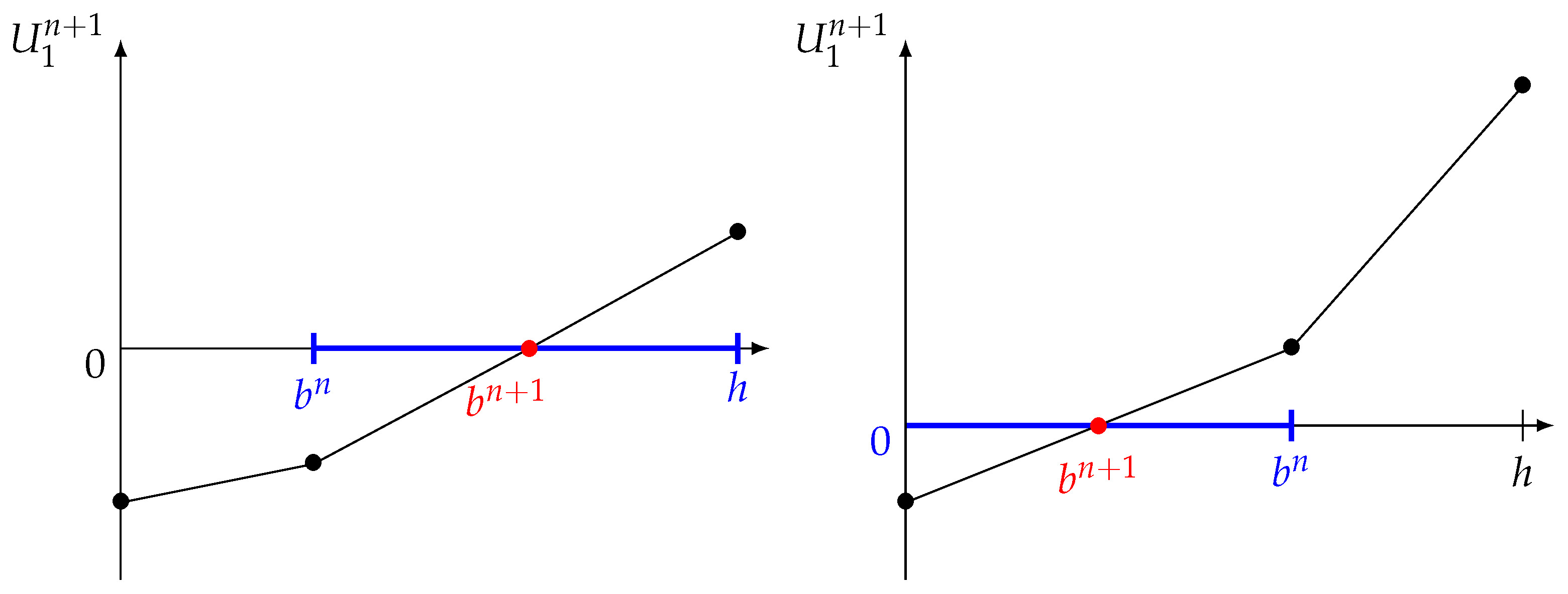
The solution to Equations (22)–(24) is obtained as follows. We can solve the system (22) together with the boundary conditions (24a) and (24c) for any value of $b^{n+1}$ since it is a linear system in $U^{n+1}$ with right-hand side containing $U^n$, the source term and the advection term (remember that the advective derivative is treated explicitly). This leads to a tridiagonal linear system with a matrix that results only from the time derivative and the diffusive terms. This matrix, which is diagonally dominant, has an inverse with nonnegative entries. Thus, the solution ${(U_j^{n+1})}_{1\le j\le n_Y}$ can be expressed linearly with nonnegative coefficients in terms of the coefficients ${(a_j^{n+1/2})}_{1\le j\le n_Y}$ which appear on the right-hand side and which depend on the still unknown interface position $b^{n+1}$. According to (23) and since $U_j^n$ is nondecreasing with respect to j (it should remain nondecreasing because we assume ${\partial }_{Z}S\le 0$), $U_j^{n+1}$ is thus, for all $j=1\dots n_Y$, a nondecreasing continuous and piecewise linear function of $b^{n+1}$, with two different formulae corresponding to whether $b^{n+1}$ is greater or smaller than $b^n$. In particular, the remaining boundary condition (24b), which is equivalent to $U_1^{n+1}=0$ owing to (24a), determines a unique solution $b^{n+1}$, see Figure 8. The value of $b^{n+1}$ can be computed explicitly by solving the linear system twice with two different right-hand sides and using linear interpolation. The first solve uses the right-hand side evaluated with the temporary value $b^n$ for $b^{n+1}$, yielding a temporary value for $U_1^{n+1}$. If the obtained value is negative (left panel of Figure 8), the second solve is performed using the value h for $b^{n+1}$, otherwise the value 0 is used (right panel of Figure 8). Once $b^{n+1}$ is known, we determine the entire profile $U_j^{n+1}$ for all $j=1\dots n_Y$ by linear interpolation.

4.2. Discretization by an Optimality Condition

The second numerical method for solving conditions (3), (4) and (5) with positive viscosity $\nu >0$ uses a formulation as an optimal problem set on the whole interval $(0,h)$, valid under the assumption ${\partial }_{Z}S(t,Z)\le 0$,

$$\left\{\begin{array}{ccc}min({\partial }_{t}U+S-{\partial }_Z(\nu {\partial }_{Z}U),U)=0\hfill & \hfill & \mathrm{for}\mathrm{all}Z\in (0,h),\hfill \\ {\partial }_{Z}U=0\hfill & \hfill & \mathrm{at}Z=h,\hfill \\ U=0\hfill & \hfill & \mathrm{at}Z=0,\hfill \end{array}\right.$$

(26)

where we consider a no-slip boundary condition at the bottom. Note that this condition becomes relevant whenever the static/flowing interface reaches the bottom, a situation encountered in our simulations as shown in Figure 10c. In (26), the static/flowing interface position $b(t)$ no longer appears explicitly, but has to be deduced from the velocity profile as

$$b(t)=inf\left\{Z\in [0,h]\mathrm{such}\mathrm{that}U(t,Z)>0\right\}.$$

(27)

We split the space domain $(0,h)$ into $n_Z$ cells of length $\Delta Z$ with $n_Z\Delta Z=h$, and denote the center of the cells by $Z_j=(j-1/2)\Delta Z$, for all $j=1\dots n_Z$. The discrete times $t^n$, for all $n\ge 0$, are related by $t^{n+1}=t^n+\Delta t^n$, where $\Delta t^n$ is the time step (chosen according to the CFL condition (30) below) and $t^0=0$. We discretize the problem (26) using a finite difference scheme by writing for the discrete unknowns $U_j^n\simeq U(t^n,Z_j)$

$$min\left(\frac{U_j^{n+1}-U_j^n}{\Delta t^n}+S(t^n,Z_j)-\frac{{\nu }_{j+1/2}^n(U_{j+1}^n-U_j^n)-{\nu }_{j-1/2}^n(U_j^n-U_{j-1}^n)}{\Delta Z^2},U_j^{n+1}\right)=0,$$

(28)

for all $j=1\dots n_Z$. The boundary conditions, which are discretized as $U_{n_Z+1}^n=U_{n_Z}^n$ at the free surface ($Z=h$) and as $U_0^n=-U_1^n$ at the bottom ($Z=0$), are used to provide the ghost values involved in the discretization of the diffusive term. The problem (28) is solved in two steps as

$$\begin{array}{c}{\displaystyle \frac{U_j^{n+1/2}-U_j^n}{\Delta t^n}+S(t^n,Z_j)-\frac{{\nu }_{j+1/2}^n(U_{j+1}^n-U_j^n)-{\nu }_{j-1/2}^n(U_j^n-U_{j-1}^n)}{\Delta Z^2}=0,}\\ {\displaystyle U_j^{n+1}=max(U_j^{n+1/2},0).\phantom{|}}\end{array}$$

(29)

Owing to the explicit discretization of the diffusive term, we use the CFL condition

$$2\underset{j}{sup}{\nu }_{j+1/2}^n\frac{\Delta t^n}{\Delta Z^2}\le 1.$$

(30)

We could also consider an implicit discretization to avoid any CFL condition, but each time step would be more computationally demanding. Finally, the thickness of the static layer can be evaluated as

$$b^n=\left(min\left\{j\in \left\{1\dots n_Z\right\}\mathrm{such}\mathrm{that}{U}_j^n>0\right\}-1\right)\times \Delta Z.$$

(31)

However, to prevent $b^n$ from being influenced by small values of U and for better accuracy, we prefer to use

$$b^n=max\left(Z_{k^n}-\sqrt{2U_{k^n}^n/C_0},0\right),k^n=min\left\{j\in \{1,\dots ,n_Z\}\mathrm{such}\mathrm{that}{U}_j^n\ge C_0\Delta Z^2/2\right\},$$

(32)

where $C_0$ is an appropriate constant of the order of $S/\nu$, in relation to Equations (4a), (4b) and (7).

In our computations, we use 200 space cells. With the value $h=0.02$ m, this leads to $\Delta Z={10}^{-4}$ m. Since $S/\nu \simeq 1.35$ ms${}^{-2}/(5\times {10}^{-5}$ m${}^2$s${}^{-1})=2.7\times {10}^4$ m${}^{-1}$s${}^{-1}$, this gives a velocity threshold of $(S/\nu )\Delta Z^2/2\simeq 1.4\times {10}^{-4}$ ms${}^{-1}$. This value is much smaller than the accuracy of experimental velocity measurements which is around 1 cm/s.

4.3. Scales in the Transient Regime

We assume that the source term S is constant, and that the viscosity $\nu$ is also constant. Then, the solution to the viscous model (3)–(5) depends on the constant S, the total thickness h, the viscosity $\nu$, the initial thickness of the static layer $b^0$, and the initial velocity profile $U^0(Z)$. We introduce dimensionless quantities, denoted by carets (hats),

$$t=\tau \widehat{t},Z=l\widehat{Z},h=l\widehat{h},b=l\widehat{b},U=u\widehat{U},$$

(33)

where $\tau$ is a time scale, l a space scale, and $u=l{\alpha }_1$ with ${\alpha }_1$ being the order of magnitude of the initial shear rate. In order to write Equation (3) in dimensionless form, we take

$$l=\nu {\displaystyle \frac{{\alpha }_1}{S}},\tau ={\displaystyle \frac{l^2}{\nu }}=\nu {\displaystyle \frac{{({\alpha }_1)}^2}{S^2}}.$$

(34)

The dimensionless equation is then

$${\partial }_{\widehat{t}}\widehat{U}+1-{\partial }_{\widehat{Z}\widehat{Z}}^2\widehat{U}=0\mathrm{for}\mathrm{all}\widehat{Z}\in (\widehat{b},\widehat{h}),$$

with boundary conditions $\widehat{U}={\partial }_{\widehat{Z}}\widehat{U}=0$ at $\widehat{Z}=\widehat{b}$ and ${\partial }_{\widehat{Z}}\widehat{U}=0$ at $\widehat{Z}=\widehat{h}$. If we take a linear initial velocity profile, this dimensionless solution $\widehat{U}$ depends only on $\widehat{h}=h/l$ and ${\widehat{b}}^0=b^0/l$. Actually, since the problem is invariant by translation in Z, the solution depends only on $(h-b^0)/l$.

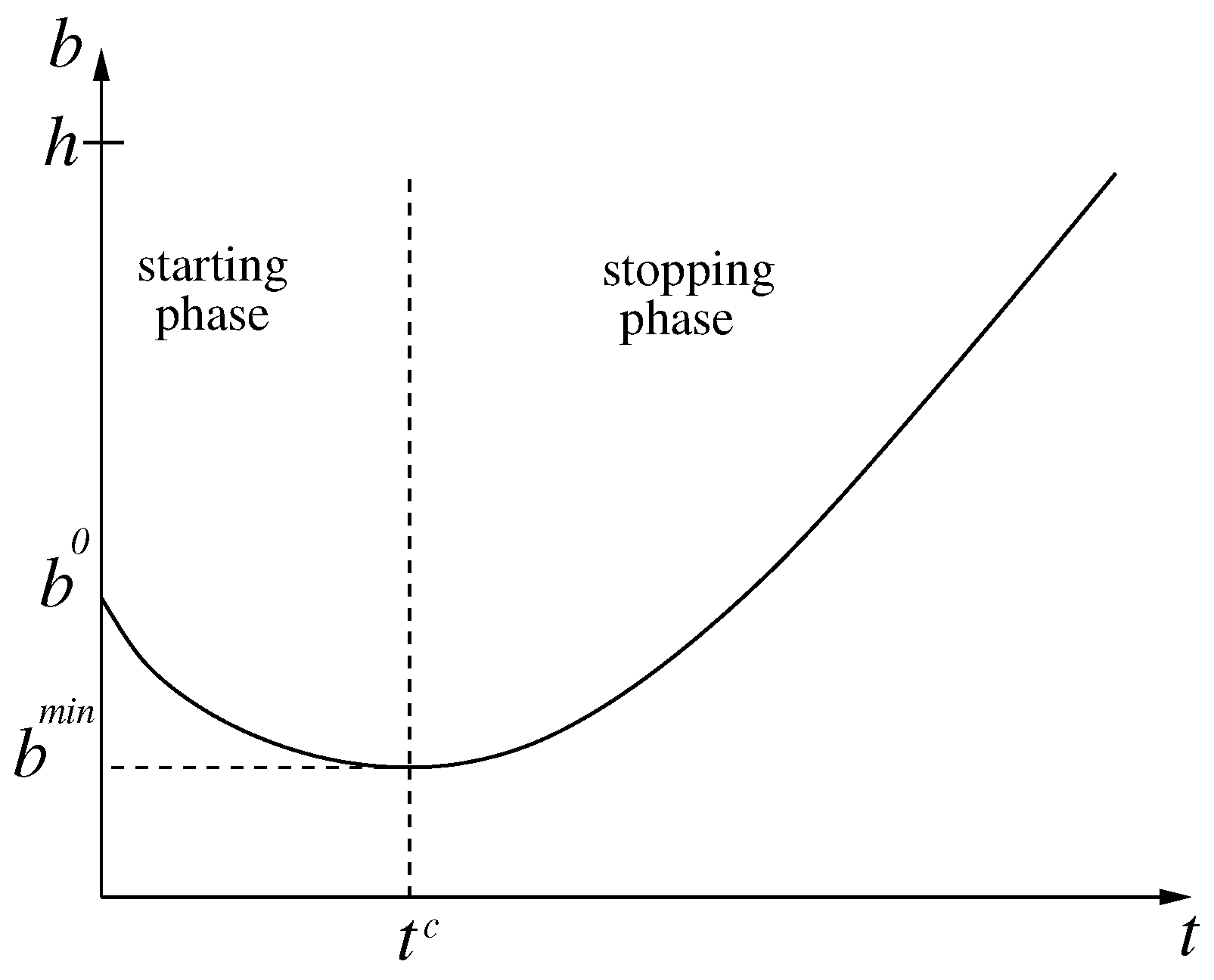
Numerical investigations for a constant source S using the scheme described in Section 4.1 show the behavior illustrated in Figure 9. The static/flowing interface position $b(t)$ first decreases until a time $t^{\mathrm{c}}$ and reaches a minimal value $b^{\min }$ (starting phase). Then $b(t)$ increases and (if h is sufficiently large) reaches an asymptotic regime with upward velocity ${\dot{b}}^{\infty }$ (stopping phase), before fully stopping when it reaches h.

According to the above scaling analysis, if the velocity profile is initially linear with shear ${\alpha }_1$, and if

$${\displaystyle \frac{h-b^0}{l}}={\displaystyle \frac{(h-b^0)S}{\nu {\alpha }_1}}\gg 1,$$

(35)

then the dimensionless problem has no parameter left and the velocity $\widehat{U}$ is therefore a fixed profile (in terms of $\widehat{Z}-{\widehat{b}}^0$), as well as $\widehat{b}-{\widehat{b}}^0$. We conclude with (33) that the quantities $t^{\mathrm{c}}$, $b^0-b^{\min }$, ${\dot{b}}^{\infty }$ are proportional to $\tau$, l, $l/\tau$, respectively. We obtain the following proportionality factors from the numerical simulation

$$t^{\mathrm{c}}=0.15\nu {\displaystyle \frac{{({\alpha }_1)}^2}{S^2}},b^0-b^{\min }=0.43\nu {\displaystyle \frac{{\alpha }_1}{S}},{\dot{b}}^{\infty }=0.95{\displaystyle \frac{S}{{\alpha }_1}}$$

(36)

Note the dependency on the ratio ${\alpha }_1/S$, which is due to the homogeneity of the problem (3) and (4) with respect to $(U,S)$ (a new solution can be obtained by multiplying $(U,S)$ by a positive constant, with b unmodified).

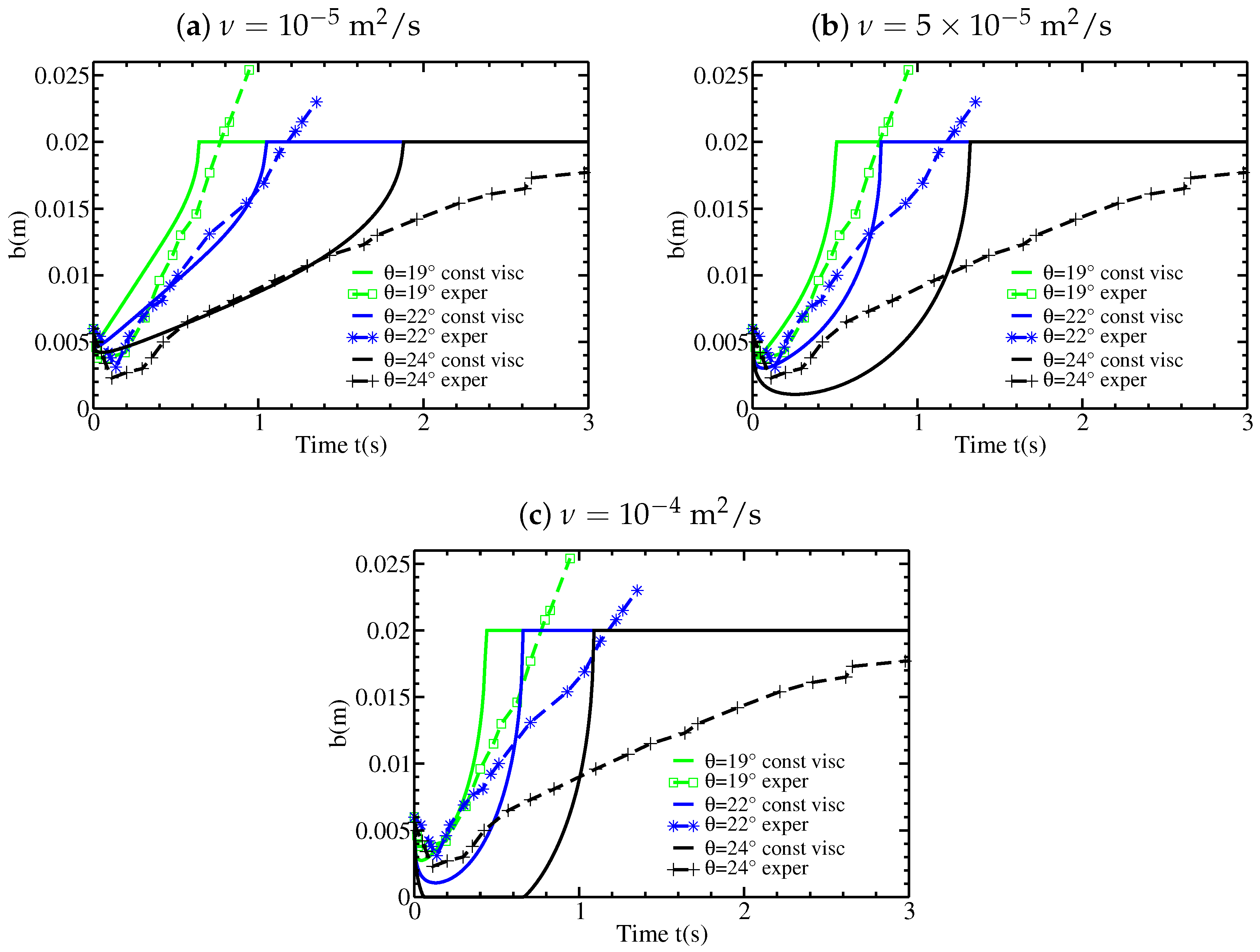
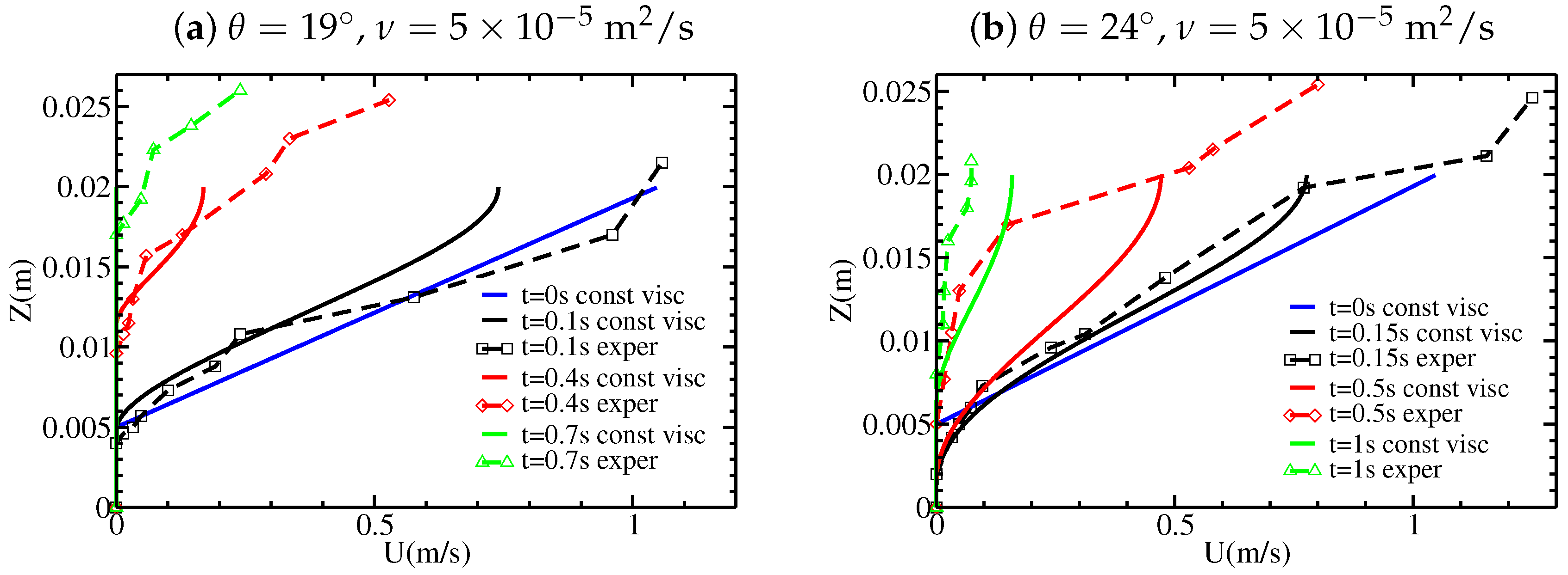
4.4. Results and Comparison with Experiments for Constant Viscosity

We consider a constant and uniform source term of the form (14). The case of a linear initial velocity profile is simulated using different values of the viscosity $\nu$ (taken constant) and slope angles $\theta$. The results obtained with the two methods of Section 4.1 and Section 4.2 are always identical, thus we shall not specify which one is used. As discussed in Section 4.3, the static/flowing interface always penetrates the initially static layer, in contrast to what has been observed for the inviscid model, within a length $b^0-b^{\min }$ proportional to $\nu$, according to (36). In other words, the flow excavates the static bed. However, for $\nu <{10}^{-5}$ m${}^2$s${}^{-1}$, the penetrating length is too small to be observed. For $\nu ={10}^{-5}$ m${}^2$s${}^{-1}$ (Figure 10a), $b^0-b^{\min }=8\times {10}^{-4}$ m for $\theta ={24}^{\circ }$ (with $t^c=5\times {10}^{-2}$ s) and $b^0-b^{\min }=2\times {10}^{-4}$ m for $\theta ={19}^{\circ }$ (with $t^c=4\times {10}^{-3}$ s). Thus, the static/flowing interface penetrates only slightly within the initially static layer. As the viscosity increases (Figure 10b), the static/flowing interface penetrates deeper into the initially static layer and even reaches the bottom for $\nu ={10}^{-4}$ m${}^2$s${}^{-1}$ at $\theta ={24}^{\circ }$ (Figure 10c). The results that best reproduce the experimental observation for the penetration of $b(t)$ within the initially static layer are obtained with $\nu \simeq 5\times {10}^{-5}$ m${}^2$s${}^{-1}$. In good agreement with the experiments, the simulations with viscosity predict that the depth and duration $t^c$ of penetration of the static/flowing interface within the initially static layer increase with the slope angle. Furthermore, the values of $b(t)$ and $t^c$ are in reasonable agreement with those observed experimentally (Figure 10b and Figure 17 of [12]).

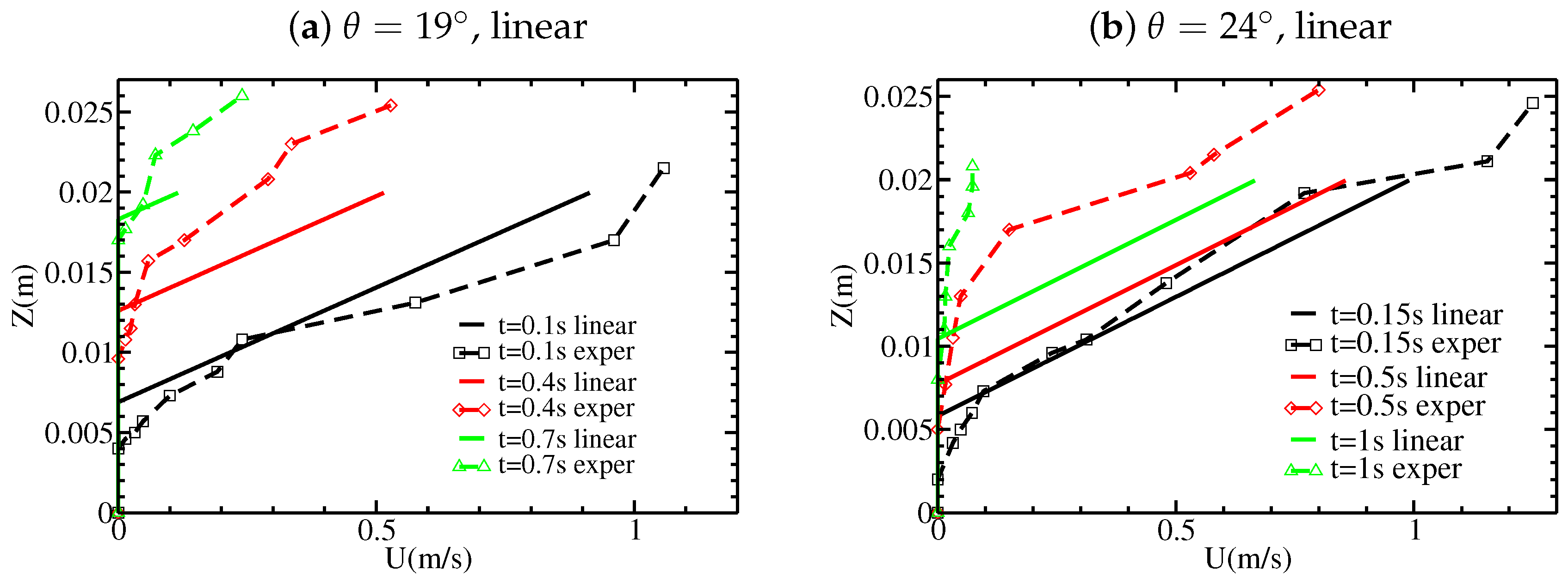
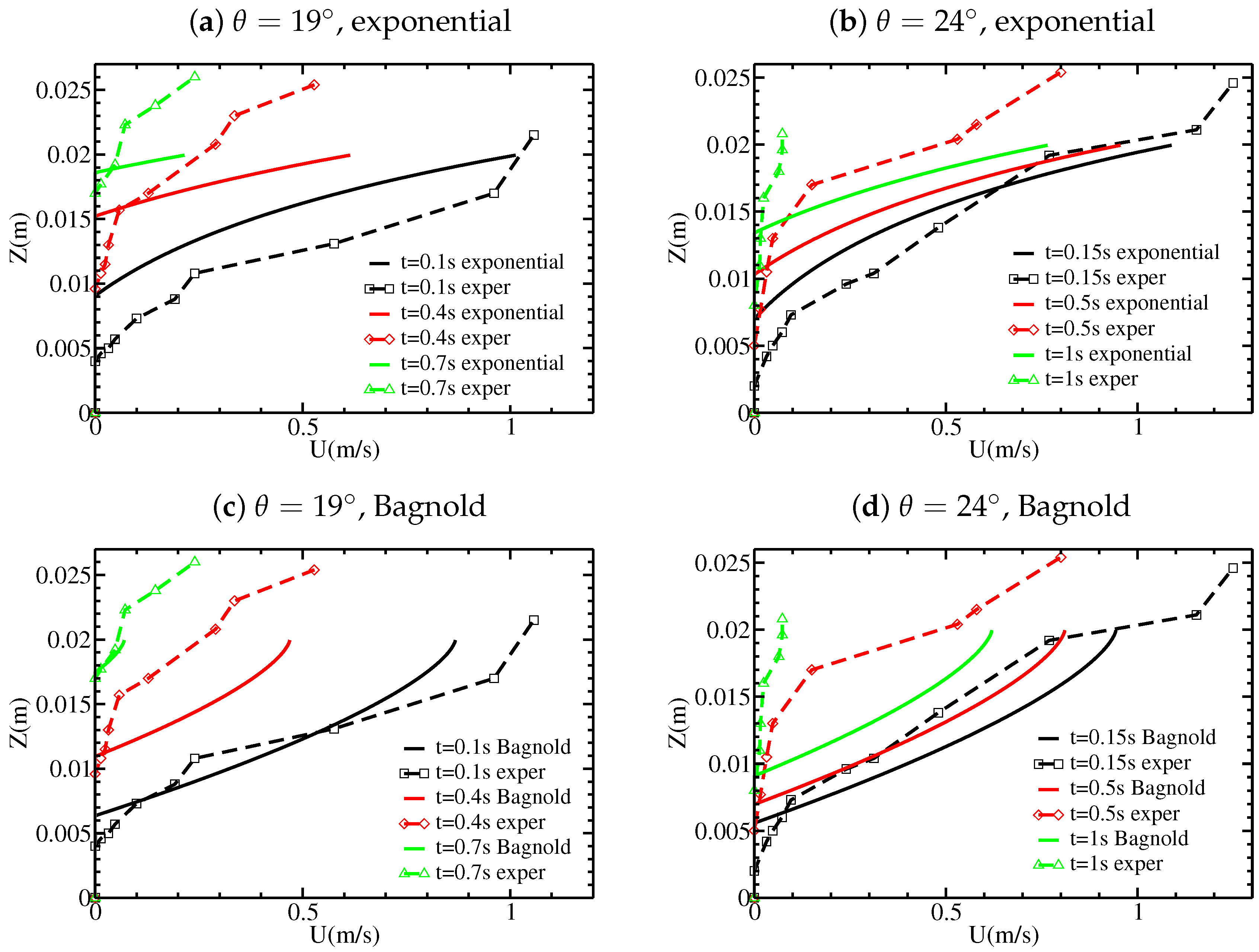
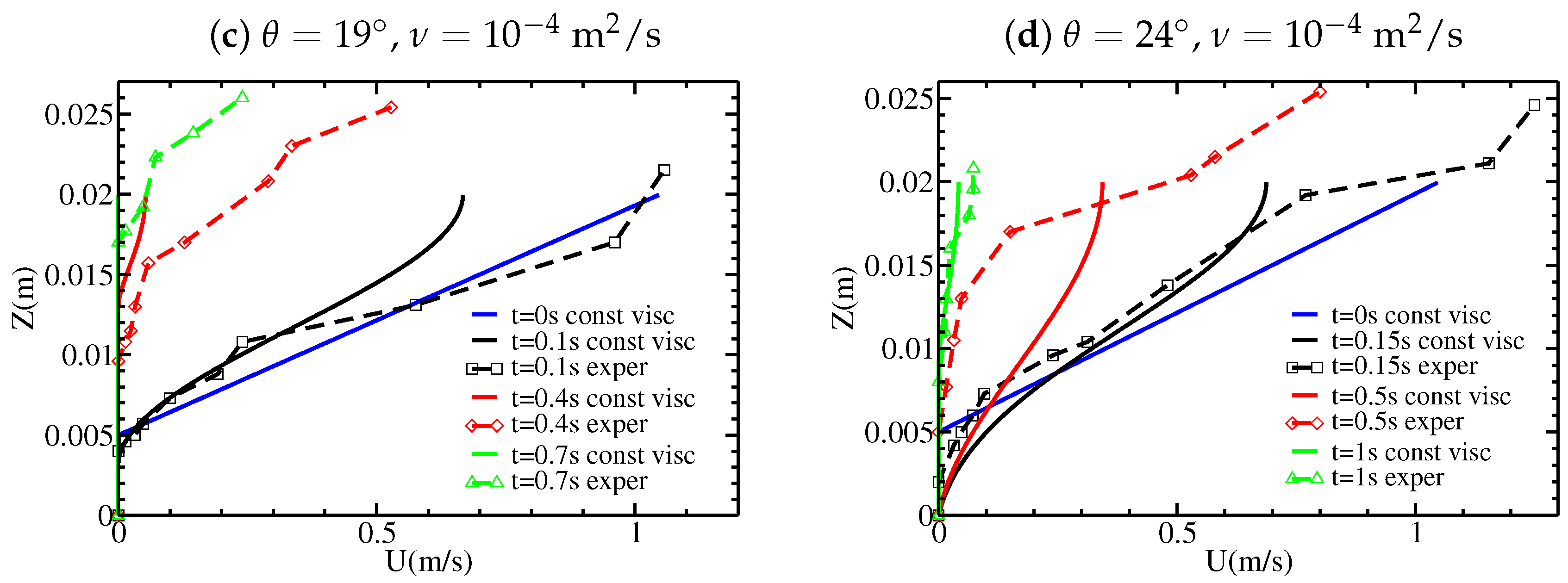
Qualitatively similar results are obtained using different initial velocity profiles (Figure 12). However, the shape of $b(t)$ is affected by the choice of the initial velocity profile. For example, for an exponential initial velocity profile with $\theta ={24}^{\circ }$ and $\nu =5\times {10}^{-5}$ m${}^2$s${}^{-1}$, the static/flowing interface position $b(t)$ stagnates at an almost constant position for the first 0.5s, contrary to the case of a linear initial velocity profile (Figure 10b and Figure 12b).

The convex shape of $b(t)$ during the migration of the static/flowing interface up to the free surface obtained with the viscous model is very different from that observed and from that obtained with the inviscid model, which predicted a linear shape related to the linear initial velocity profile. With the viscous model, the time evolution of $b(t)$ and the velocity profile $U(t,Z)$ are not so clearly related to the shape of the initial velocity profile, as shown for example in Figure 12 for $\theta ={24}^{\circ }$. The velocity profiles for the viscous model are also very different from those for the inviscid model. Whatever the shape of the initial velocity profile, the velocity profiles later exhibit an exponential-like tail near the static/flowing interface, similar to that observed experimentally. They also exhibit a convex shape near the free surface which can be observed, although not as marked, in some but not all experimental velocity profiles (e.g., Figure 3c). While the maximum velocity decreases too fast at $t=0.5$ s and $\theta ={24}^{\circ }$ compared to the experiments and to the inviscid model, the velocity is much closer to the experiments at $t=1$ s than with the inviscid model (Figure 11b). For $\theta ={19}^{\circ }$ and $\theta ={22}^{\circ }$, the decrease in velocity at time $t=0.7$ s is overestimated in the viscous model.

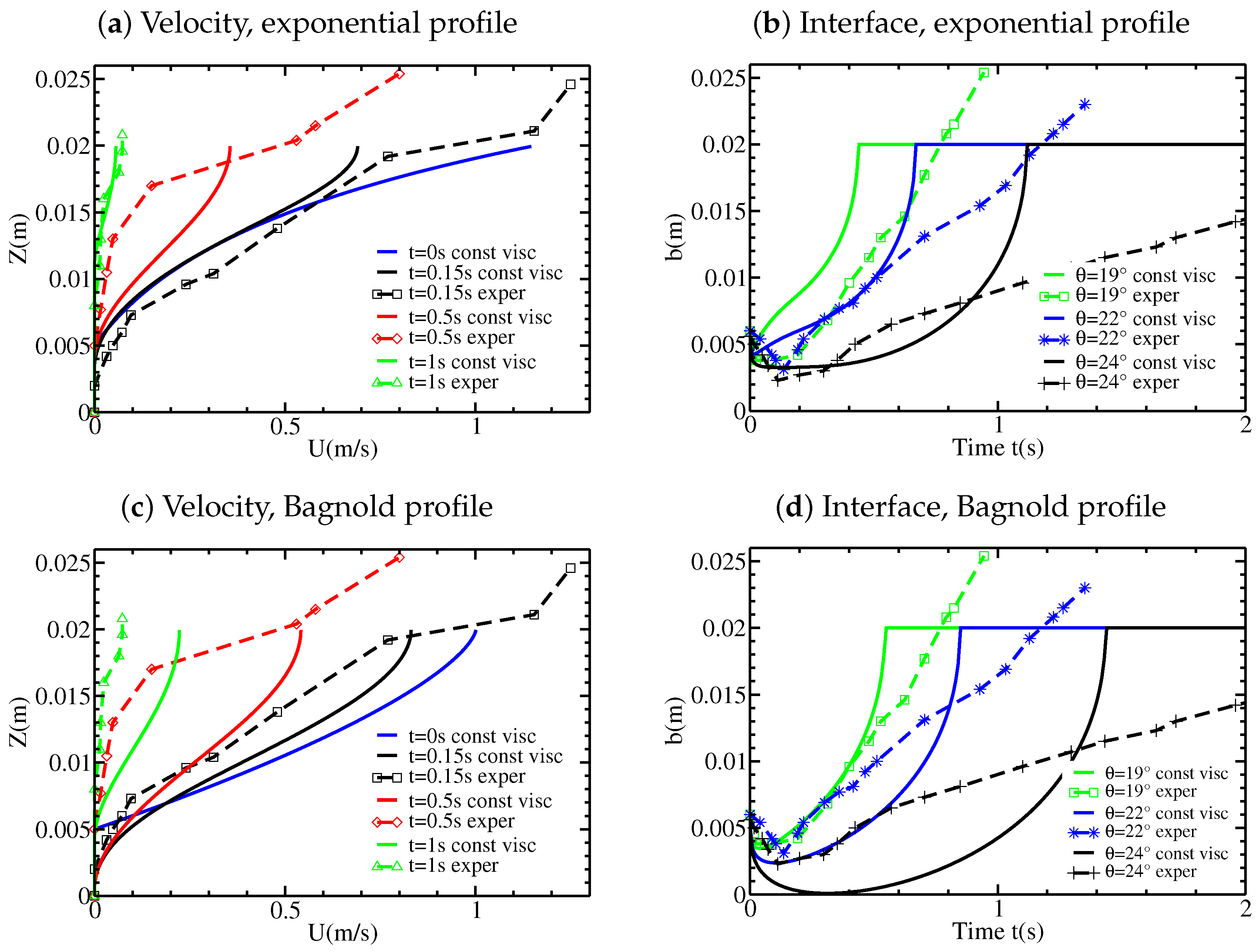
Finally, we briefly look at the stopping time $t^{\mathrm{stop}}$ of the whole granular layer. The stopping time for the inviscid model and for the experiments is given in

Table 1. Stopping time $t^{\mathrm{stop}}$ for the inviscid model $t_{\nu =0}^{\mathrm{stop}}=U^0(h)/S$ (for linear initial velocity profile) and in the experiments (from Figure 2), for different slope angles.

${\mathit{t}}^{\mathbf{stop}}$ (s)	$\mathit{\theta }={\mathbf{19}}^{\circ }$	$\mathit{\theta }={\mathbf{22}}^{\circ }$	$\mathit{\theta }={\mathbf{24}}^{\circ }$
inviscid model	$0.79$	$1.4$	$2.8$
experiments	$0.94$	$1.3$	$3.3$

, for different slope angles. The stopping time is smaller for viscous than for inviscid flow, whatever the shape of the initial velocity profile. Given that the stopping time for the inviscid model is expressed as $t_{\nu =0}^{\mathrm{stop}}=U^0(h)/S$, we can evaluate numerically the difference $(t_{\nu =0}^{\mathrm{stop}}-t_{\nu }^{\mathrm{stop}})$, where $t_{\nu }^{\mathrm{stop}}$ denotes the stopping time for the viscous model. Our numerical simulations show that this difference depends to a moderate extent on the viscosity (Figure 13 where the slope of the curves suggests a behavior of this difference close to ${\nu }^{1/4}$ for the present parameters). In any case, the presence of viscosity diminishes the stopping time. Consequently, according to Table 1, the stopping time is significantly smaller in the viscous model than in the experiments. This can also be observed in Figure 10 and Figure 12 (right).

4.5. Variable Viscosity

The viscoplastic description of granular materials involves fundamentally a Drucker-Prager yield stress proportional to the pressure, the coefficient being the static friction parameter ${\mu }_s=tan\delta$. A full rheological law including this yield stress (i.e., defined for all values of the strain rate and not only close to zero) has been proposed in [28], the so called $\mu (I)$ rheology. As described in [32], this rheology can be interpreted as a decomposition (i.e., (2)) of the deviatoric stress tensor in a rate-independent pure plastic part proportional to ${\mu }_s$ and a viscous part with pressure- and rate-dependent dynamic viscosity $\eta$ given by

$$\eta =(\mu (I)-{\mu }_s)\frac{p_{dyn}}{2\parallel D\parallel },$$

(37)

where $p_{dyn}$ is the dynamic pressure, D is the strain rate tensor, ${\parallel D\parallel }^2=\frac{1}{2}{\sum }_{ij}{D}_{ij}^2$, and I is the inertial number defined by

$$I=\frac{2\parallel D\parallel d}{\sqrt{p_{dyn}/{\rho }_s}},$$

(38)

with d the grain diameter as before and ${\rho }_s$ the grain density. The kinematic pressure p is related to $p_{dyn}$ by $p=p_{dyn}/\rho$, with $\rho =\varphi {\rho }_s$ the density of the granular material, $\varphi$ being the volume fraction. If we consider a slope aligned velocity field depending only on the normal coordinate Z (simple shear flow), the arguments of Section 2.3 show that the solution to the viscoplastic model (1) and (2) is described by the system (3)–(5) with the constant and uniform source term S given by (14) and $\nu =\eta /\rho$. Such a flow has hydrostatic pressure $p=gcos\theta (h-Z)$ and shear rate $\parallel D\parallel ={\partial }_{Z}U/2$. Thus with (37), the kinematic viscosity becomes

$$\nu =(\mu (I)-{\mu }_s)\frac{gcos\theta (h-Z)}{{\partial }_{Z}U},$$

(39)

with

$$I=\frac{{\partial }_{Z}Ud}{\sqrt{\varphi gcos\theta (h-Z)}}.$$

(40)

Then the term appearing in (3) is

$$\nu {\partial }_{Z}U=(\mu (I)-{\mu }_s)gcos\theta (h-Z),$$

(41)

and the part of this term proportional to ${\mu }_s$ indeed balances in (3) the corresponding part in S from (14). The nonlinearity is given according to [28] as

$$\mu (I)={\mu }_s+({\mu }_2-{\mu }_s)\frac{I}{I+I_0},$$

(42)

with ${\mu }_2>{\mu }_s$ the friction at large strain rate and $I_0$ is a constant that depends on the material used and other device specificities, see ([27], Appendix A). Here we take the value $I_0=0.279$ proposed by [27]. Note that the boundary condition (4c) is automatically satisfied and can therefore be skipped.

For the discretization, we use the method of Section 4.2 with the discrete unknowns $U_j^n\simeq U(t^n,Z_j)$, $Z_j=(j-1/2)\Delta Z$ for $j=1\dots n_Z$, $n_Z\Delta Z=h$. The Equations (3) and (41) with (42) and (40) are discretized with finite differences under the conservative form

$$\frac{U_j^{n+1/2}-U_j^n}{\Delta t^n}+S(t^n,Z_j)-\frac{{\mathrm{\Phi }}_{j+1/2}^n-{\mathrm{\Phi }}_{j-1/2}^n}{\Delta Z}=0,$$

(43)

for all $j=1\dots n_Z$, with

$${\mathrm{\Phi }}_{j+1/2}^n=(\mu (I_{j+1/2})-{\mu }_s)gcos\theta (h-Z_{j+1/2}),I_{j+1/2}=\frac{d(U_{j+1}^n-U_j^n)/\Delta Z}{\sqrt{\varphi gcos\theta (h-Z_{j+1/2})}}$$

(44)

for $j=0\dots n_Z$, with $Z_{j+1/2}=Z_j+\Delta Z/2=j\Delta Z$, and once $U_j^{n+1/2}$ has been computed, we set

$$U_j^{n+1}=max(U_j^{n+1/2},0).$$

(45)

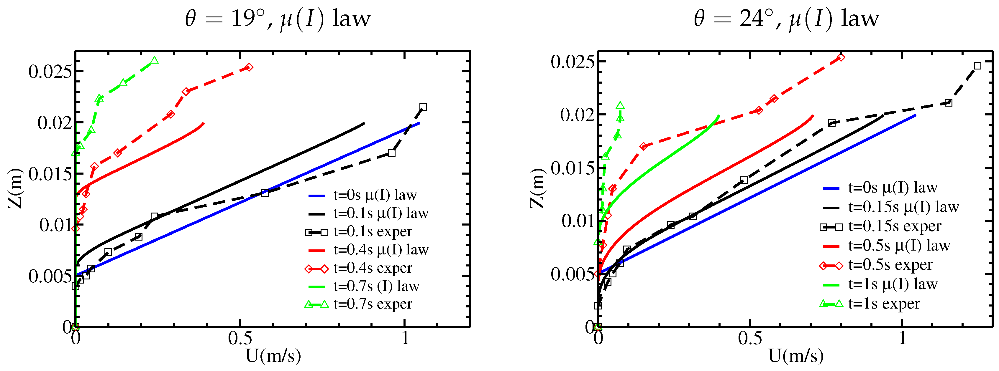
Since ${\mathrm{\Phi }}_{n_Z+1/2}^n=0$, there is no need to define $U_{n_Z+1}^n$, in accordance with the loss of the free surface boundary condition (4c). On the left boundary (bottom), we use as before the no-slip condition, $U_0^n=-U_1^n$. We use the CFL condition $2{\nu }_{\max }\Delta t^n\le \Delta Z^2$, with ${\nu }_{\max }$ defined as the maximum value of $\nu$ computed with (39). The interface position $b^n$ is computed according to (32).

As previously, we take ${\mu }_s=tan({26}^{\circ })$, $h=0.02$ m, $b^0=0.005$ m, and $d=7\times {10}^{-4}$ m. As in [12], we take $\varphi =0.62$. We choose ${\mu }_2=tan({28}^{\circ })$, which leads to $\nu (Z=b^0)\simeq 5\times {10}^{-5}$ m${}^2$s${}^{-1}$, corresponding to the order of magnitude of $\nu$ taken in Section 4.4. We consider the case of a linear initial velocity profile, with slope angles $\theta ={19}^{\circ },{22}^{\circ },{24}^{\circ }$. The numerical results for the static/flowing interface position $b(t)$ and velocity profiles $U(Z)$ are plotted in Figure 14 and Figure 15. In comparison with numerical results of Figure 10b and Figure 11a,b obtained with the constant viscosity model, the shapes are similar, in particular for the initial erosion of the static bed. The behavior of the interface position $b(t)$ reaching the free surface close to the stopping time is here closer to the prediction of the inviscid model (see Figure 5a). However, this behavior does not recover (since $\nu$ vanishes at the free surface) the expected behavior, which is roughly linear, of the experimental results of Figure 2. The comparison with the experimental results is better with the $\mu (I)$ rheology than with a constant viscosity. For clarity, the static/flowing interfaces and the velocity profiles corresponding to the different cases are plotted in Figure 16 for $\theta ={22}^{\circ }$.

It is important to explain the behavior of the solution close to the free surface. As said above, there is no need to impose any boundary condition at the free surface, because the pressure vanishes there. Nevertheless, the behavior close to the free surface of the solution to the parabolic problem (3) is deduced from the property that ${\partial }_Z(\nu {\partial }_{Z}U)$ is bounded, which gives $\nu {\partial }_{Z}U\sim h-Z$. For the model with constant viscosity, this leads to ${\partial }_{Z}U\sim h-Z$ and U has a (rather) parabolic profile close to the free surface. For the model with $\mu (I)$ rheology, Equation (41) implies that I tends to a finite value as $Z\to h$, and thus with Equation (40), we obtain ${\partial }_{Z}U\sim \sqrt{h-Z}$, and U has a (rather) Bagnold profile close to the free surface. We conclude that in any case, the Neumann condition ${\partial }_{Z}U=0$ is recovered at the free surface, even if not enforced explicitly. For the model with the $\mu (I)$ rheology, ${\partial }_{Z}U$ tends to zero more slowly than for the model with constant viscosity, leading to a behavior closer to the prediction of the inviscid model. Nevertheless, the property ${\partial }_{Z}U=0$ at the free surface, which seems to be a consequence of the incompressible viscoplastic model, makes it impossible to obtain a good representation of the experimental stopping phase.

Note that the $\mu (I)$ rheology was introduced precisely to represent the Bagnold profile (without a static phase) $U(Z)=c(h^{3/2}-{(h-Z)}^{3/2})$, where c is determined by the relation $\mu (I)=tan\theta$, which gives

$$c=\frac{2}{3}\frac{I_0}{d}\frac{tan\theta -{\mu }_s}{{\mu }_2-tan\theta }\sqrt{\varphi gcos\theta }.$$

(46)

This Bagnold profile without a static phase is a steady solution to the system (3) and (41) with (42) and (40), but only when ${\mu }_s<tan\theta <{\mu }_2$. In our framework, we have a static phase, the flow is not steady, and $tan\theta <{\mu }_s$. The formula (46) is therefore not applicable and would give a negative c. Our choice of ${\alpha }_3$ is nevertheless of the same order of magnitude as formula (46).

5. Discussion and Conclusions

We have considered the 1D (in the direction normal to the flow) non-averaged model with static/flowing dynamics that was initially proposed in [41]. This model is based on the description of a granular material by a yield stress viscoplastic rheology. Here we have assumed that the source term in this model is constant, which corresponds to simple shear solutions to the viscoplastic model. Thus, all the quantities are assumed to be independent of the down-slope variable and in particular the flow thickness is constant. We have shown that this free interface model can be solved with reliable and relatively simple numerical methods. We have compared model solutions for both the inviscid and viscous models to observations from experiments on granular flow over an inclined static layer of grains. The analytical solution for the inviscid model and the numerical results for the viscous model reproduce quantitatively some essential features of the change with time of the velocity, of the static/flowing interface position, and of the stopping time of the granular mass, even though the flow thickness in the experiments is not perfectly uniform and the initial velocity profile changes with slope angle and flow thickness as discussed below.

The analytical solution for the inviscid model shows that the evolution of the static/flowing interface position is proportional to the source term and inversely proportional to the shear rate (Equation (9)). For the viscous model (with constant viscosity), the analysis shows that the evolution of the interface is related to the viscosity, the source term, and the first- and third-order derivative of the source term and the velocity, respectively (Equation (8)). Owing to the appearance of this third-order derivative, the dynamics of the static/flowing interface cannot be reduced to a simple differential equation in terms of depth-averaged quantities. While the shape of the initial velocity profile is preserved at all times for the inviscid model according to Equation (15), the viscous model predicts that an exponential-like tail near the static/flowing transition and a convex shape near the free surface develop. The viscous contribution enables the static/flowing interface to initially penetrate within the static layer (which is eroded), as observed in the experiments, and contrary to the inviscid model.

The viscoplastic model used here has the great advantage of involving only two parameters, i.e., the friction coefficient ${\mu }_s$ and the viscosity $\nu$ (or the coefficient ${\mu }_2$ for the $\mu (I)$ rheology), whereas the so-called partial fluidization theory, involving an order parameter to describe the transition between static and flowing material, also reproduces the erosion of the static bed and the velocity profiles predicted here with the viscous model [7], but at the cost of additional empirical equations for the time-change of a state parameter.

One of the important results of the analysis lies in the explicit expressions obtained from the analytical solution, especially for the time evolution of the static/flowing interface. The dynamics are controlled by the source term S that is constant when the pressure is assumed to be hydrostatic and when the slope and thickness are assumed to be constant. In such a case, $S(t,Z)=S=gcos\theta (tan\delta -tan\theta )$, with ${\mu }_s=tan\delta$. Comparable results have been obtained from the analytical solution of thin-layer depth-averaged equations for a granular dam-break (i.e., with non-constant h) [43,44]. This analytical solution predicts a granular mass front velocity that decreases linearly with time

$$U_f=max\left(2\sqrt{kg{h}_{0}cos\theta }-\left(gcos\theta (tan\delta -tan\theta \right)t,0\right),$$

(47)

where $k\simeq 0.5$ (see [9]). Furthermore, the stopping time of the analytical front for the granular dam-break is

$$t_f=2\sqrt{\frac{k{h}_0}{gcos\theta }}\frac{1}{tan\delta -tan\theta }.$$

(48)

Equations (47) and (48) for the front velocity and the stopping time of the front for a depth-averaged model of a granular dam-break are very similar to Equations (15) and (17) respectively, found here for the velocity of the flow and for the stopping time of the granular layer in the non-averaged case and without viscosity.

Although the initial penetration of the static/flowing interface into the static layer (erosion) can be reproduced by taking into account the viscosity, this leads at the same time to an underestimation of the stopping time. The viscous model better reproduces the exponential-like tail of the velocity profile near the static/flowing interface than the inviscid model, but overestimates the convexity of the velocity profile near the free surface. Furthermore, the change in shape of the velocity profile observed in the experiments during the stopping phase is reproduced by the viscous model, as opposed to the inviscid model. However, the decrease in maximum velocity near the surface is too fast in the viscous model. All these results suggest that (i) viscosity plays an important role near the static/flowing interface at depth and in this region a reasonable estimate for the viscosity is $\nu \simeq 5\times {10}^{-5}$ m${}^2$s${}^{-1}$ and (ii) viscous effects in the experiments seem to be much smaller near the free surface. These observations suggest a non-constant viscosity, as proposed in the so-called $\mu (I)$ flow law, e.g., [25,26,27,28]. As in [32], we have used the $\mu (I)$ flow law to derive the value of the viscosity, which becomes variable and nonlinear with respect to the shear rate. This flow law reproduces approximately the value of the viscosity at the static/flowing interface (i.e., $\nu \simeq 5\times {10}^{-5}$ m${}^2$s${}^{-1}$) and at the free surface (vanishing viscosity). However, this model does not allow us to significantly improve the accuracy of the behavior of the static/flowing interface close to stopping. This is because it imposes a Bagnold behavior close to the free surface, which is in contradiction with experiments that predict a linear behavior. A more detailed numerical simulation of the granular collapse over sloping beds with the complete viscoplastic model and the $\mu (I)$ rheology gives a dynamic viscosity of around 0.2Pa· s near the front, increasing up to about 0.4Pa·s behind the front (see Figure 11 of [33] and Figure 10 of [32]), leading to a kinematic viscosity of $\nu =1.3\times {10}^{-4}$ m${}^2$s${}^{-1}$ and $\nu =2.6\times {10}^{-4}$ m${}^2$s${}^{-1}$, respectively, for a density of $\rho =1550$ kg/m${}^3$. Note also that our treatment of side wall effects deserves further improvements, since we simply increased the friction coefficient as done in [27,32,42]. Taking into account wall effects changes the static/flowing position, as shown in particular in [33] for the granular collapse considered here. More precisely, the static/flowing interface is found to be less deep within the flow when wall effects are accounted for (see Figures 3 and 4 of [33]). This effect could possibly increase the value of the viscosity needed in the model to reproduce the penetration of the static/flowing interface observed in the experiments. This would give values of the viscosity closer to that given by the $\mu (I)$ rheology near the front (Figure 11 of [33]).

It would be of interest to take into account the X-variations of the source S from ([41], Equation (2.12)), thereby accounting for topography, propagation and non-hydrostatic effects. This would make it possible to study erosion in flows over complex topography in the laboratory (e.g., [45]) or at the natural scale (e.g., [46]). For the very simple case of flows over a constant slope and if the pressure is assumed to be hydrostatic ($p=gcos\theta (h-Z)$), taking into account the X-variations is the same as (according to [41]) considering once again (3)–(6) with S including an additional term,

$$S=gcos\theta \left(tan\delta -tan\theta +{\partial }_{X}h\right),$$

(49)

and as considering a thickness $h=h(t,X)$ that evolves according to (2.2) in [41]. Then $U=U(t,X,Z)$ and $b=b(t,X)$. However $S=S(t,X)$ in (49) is still independent of Z. Then Equations (8) and (9) read as follows with $S(t,X)$ defined by (49):

• If $\nu >0$ and $S(t,X)\ne 0$, then

  $$\dot{b}(t,X)={\displaystyle \frac{-{\partial }_{ZZ}^2(\nu {\partial }_{Z}U)(t,X,b(t))}{S(t,X)}}\nu .$$

  (50)
• If $\nu =0$ and ${\partial }_{Z}U(t,X,b(t))\ne 0$, then

  $$\dot{b}(t,X)={\displaystyle \frac{S(t,X)}{{\partial }_{Z}U(t,X,b(t))}}.$$

  (51)

The model with $0<b<h$ is valid as long as $S(t,X)\ge 0$, so as to satisfy (6). Indeed, violating this condition leads to instantaneous flow of the whole layer i.e., $b=0$, and full erosion of the bed. In this case, (3) still has to be solved (with $b=0$ and $S<0$), but with boundary conditions (4a) and (4c) only. If at some later time S becomes positive again, b can rise above the value $b=0$. 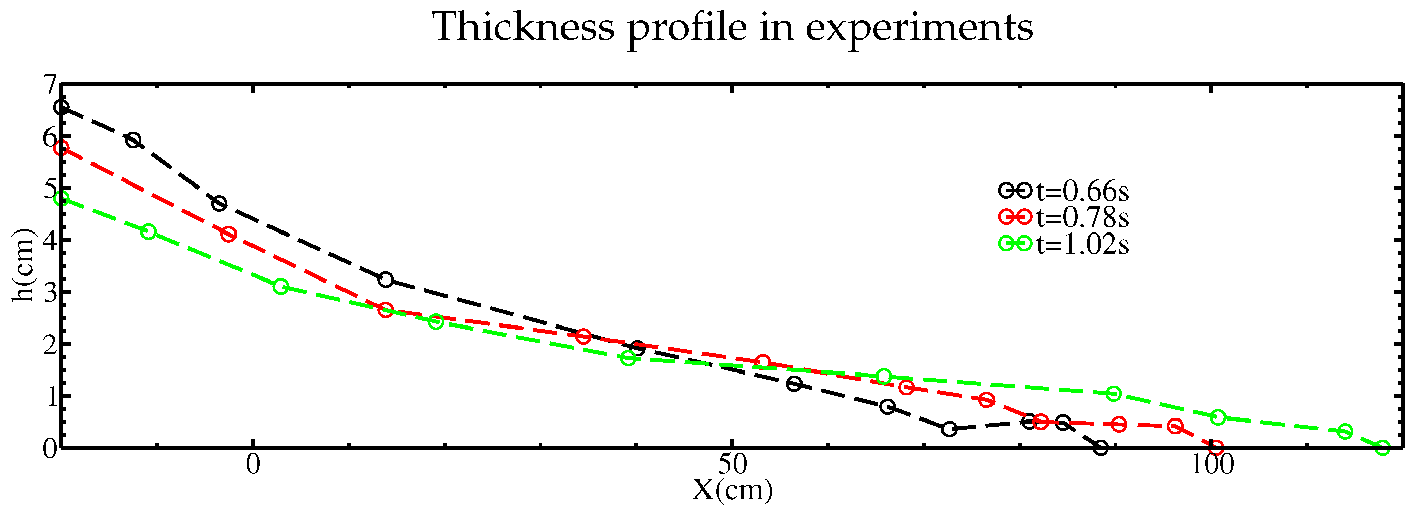Thus when $S(t,X)$ can change sign, there is in general a succession of progressive depositions and sudden full erosions of the bed. As discussed previously, the experimental granular flow is not perfectly uniform, as illustrated for example for the granular collapse at $\theta ={22}^{\circ }$ in Figure 17. In this case, $tan\delta -tan\theta =0.0837$, so that near the front, where the h-gradient is strongest (${\partial }_{X}h(t=0.66$s$,X=90$cm$)\simeq 0.125$ as shown in Figure 17), S is negative and thus even the inviscid model predicts that erosion occurs. Later, when the front flows beyond the position $X=90$ cm, ${\partial }_{X}h$ decreases with values around $\simeq 5\times {10}^{-3}$. Therefore S becomes positive, and with the inviscid model, the static/flowing interface rises (i.e., deposition occurs). For the viscous model, for the case $S\ge 0$ studied in this paper, occurrence of erosion ($\dot{b}<0$) or deposition ($\dot{b}>0$) is related according to (50) to the change of sign of ${\partial }_{ZZ}^2(\nu {\partial }_{Z}U)(t,X,b(t))$, i.e., positive and negative, respectively. Therefore, when the X variations are considered and under the hydrostatic assumption, the occurrence of erosion or deposition depends on the signs of both S and ${\partial }_{ZZ}^2(\nu {\partial }_{Z}U)(t,X,b(t))$.

The influence of a Z-dependency of S on the static/flowing interface dynamics and on the erosion process in the free interface model (3)–(6) is studied in [41]. It would be interesting to extend the approach proposed here to 2D and possibly 3D, so as to capture the static/flowing interface in thin-layer models, as proposed in [40]. The orders of magnitude assumed in [40] are indeed satisfied in the experiments discussed here, because the typical length is $L=1$ m, the typical time is $\tau =0.33$ s, (so that $L/{\tau }^2=g$), $h=0.02$ m, and $\nu =5\times {10}^{-5}$ m${}^2$s${}^{-1}$, leading to $\epsilon \equiv h/L=0.02$, $tan\delta -tan\theta =O(\epsilon )$, and the normalized viscosity $\nu \tau /L^2\simeq {10}^{-5}$ is of the order of ${\epsilon }^2$ or ${\epsilon }^3$. The primary models of [40] with dependency on X and without hydrostatic assumption (giving S depending also on Z) lead however to severe nonlinearities and ill-posedness, so that the numerical treatment of these extensions with all flow-aligned variations represents a major challenge.

An important issue is also to summarize the dynamics of the normal velocity profile using a finite number of parameters (for example the interface position b, the thickness h, and the shear rate), in order to keep computational costs low enough to simulate natural situations. This could lead to a depth-averaged model, which has until now seemed inaccessible because of the dependency on the third normal derivative in the differential Equation (8).