Excitation of Surface Waves Due to Thermocapillary Effects on a Stably Stratified Fluid Layer

1
Department of Chemical and Biological Engineering, Mappin Street, University of Sheffield, Sheffield S1 3JD, UK
2
School of Mathematics and Statistics, Hounsfield Road, University of Sheffield, Sheffield S3 7RH, UK
*
Author to whom correspondence should be addressed.
†
These authors contributed equally to this work.
Appl. Sci. 2017, 7(4), 392; https://doi.org/10.3390/app7040392
Submission received: 23 February 2017
/
Revised: 1 April 2017
/
Accepted: 10 April 2017
/
Published: 13 April 2017
(This article belongs to the Special Issue Heat Transfer Processes in Oscillatory Flow Conditions)
Abstract
:In chemical engineering applications, the operation of condensers and evaporators can be made more efficient by exploiting the transport properties of interfacial waves excited on the interface between a hot vapor overlying a colder liquid. Linear theory for the onset of instabilities due to heating a thin layer from above is computed for the Marangoni–Bénard problem. Symbolic computation in the long wave asymptotic limit shows three stationary, non-growing modes. Intersection of two decaying branches occurs at a crossover long wavelength; two other modes co-exist at the crossover point—propagating modes on nascent, shorter wavelength branches. The dispersion relation is then mapped numerically by Newton continuation methods. A neutral stability method is used to map the space of critical stability for a physically meaningful range of capillary, Prandtl, and Galileo numbers. The existence of a cut-off wavenumber for the long wave instability was verified. It was found that the effect of applying a no-slip lower boundary condition was to render all long waves stationary. This has the implication that any propagating modes, if they exist, must occur at finite wavelengths. The computation of 8000 different parameter sets shows that the group velocity always lies within to of the longwave phase velocity.
1. Introduction
Marangoni–Bénard convection still generates much interest in fluid and nonlinear dynamics due to its complexity. When the fluid layer is heated from below, convective instabilities can be driven by surface or buoyancy forces [1]. The role of surface-tension gradients in inducing convective instability through Marangoni stresses at the air–liquid interface in a thin layer initially at rest, heated from below, was characterized in the seminal works of Sternling and Scriven [2] and Smith [3] and the role of surface deformation and surface tension gradients in the onset of patterned convection and oscillatory instability is reviewed in [4].
When the layer is heated from above, however, only overstability can be excited at sufficiently high Marangoni or Rayleigh (buoyancy) numbers. The most common chemical engineering context for a cold liquid heated from above is a condenser, which comprises a hot vapor that condenses over a colder liquid chilled from the solid support below. There are many different configurations for condensers, but all of them would condense faster if interfacial waves are excited on the interface. Thus, a stability theory that shows under what conditions self excitation occurs could better inform the design and operation of condensers. The scenario also describes an evaporator that is operated by contacting hot gas over the cold liquid, as long as there is no fluid motion imposed. Of course, imposing fluid motion adds additional complication but has been found to accelerate performance in novel contactors (evaporators, condensers and distillers) [5].
Classical experiments by Linde and coworkers [6] demonstrate a series of wave instabilities excited at high Marangoni numbers, although they could not discern whether the excited waves were surface or internal waves. It was later posited that the waves were surface manifestations of soliton solutions to a dissipative variation of the Korteweg–de Vries equation. Experiments have shown that solitary waves, excited and sustained by Marangoni stresses, undergo interactions and collisions that return the waves to the pre-collision celerities and shapes, experiencing at most a phase shift, but with either sense possible [7]. Nepomnyashchy and Velarde [8] demonstrated via multiple scale perturbation methods the definitive derivation of the dissipative nonlinear evolution equation (termed the KdV–KSV equation) in a sufficiently thin layer that buoyancy effects are neglected. Their study assumed a stress-free lower boundary. The KdV–KSV theory predicts a critical Marangoni number , irrespective of capillary, Prandtl and gravity numbers. The interpretation of this result is simply that surface-tension gradients, if sufficiently strong, overcome viscous dissipation in the surface layer to start the fluid oscillations. These oscillations must then combine two modes—the gravity waves modified by Marangoni stresses that are normal to the surface (termed transverse waves) and elastic-like waves that are tangential to the surface (termed longitudinal waves). A study of solutocapillary Marangoni-induced interfacial waves is given in [9].
The purpose of this paper is to test the regime of validity of the KdV–KSV theory on two points—(i) the assumption of the multiple scale theory that there is a long wave cut-off for a wave-packet of unstable waves just above critical stability; (ii) the affect of the no-slip lower boundary on the coefficients of the linear terms of the KdV–KSV equation—by computing the full linear stability theory (LST) of the Bénard–Marangoni problem when heated from above. Since, in the basic state, the fluid is at rest and only the static pressure among the field variables has a vertical dependency, it is possible to formulate the analytic solution to the linearized equations and subsequently the secular equation for excitation of non-trivial solutions for the streamfunction, temperature, and surface displacement. The analysis presented is a precursor to the weakly nonlinear theory for the evolution of capillary gravity waves given in [10]. The model equations are presented in Section 2. In Section 3, the linear stability of both the stress-free model and the no-slip models are formulated. In each case, the long wave asymptotic forms are computed for branches of the dispersion relation found. Results are discussed in Section 4 and the conclusions are drawn in Section 5.
2. Flow Specification
2.1. Scaling
Consider a layer of viscous fluid with dynamic viscosity , density , and thermal diffusivity , which is heated from above. The background no flow and no deformation state is perturbed, giving rise to gravity, capillary, and Marangoni forces. The relevant physical parameters are summarized below:
- Surface tension where is the surface tension at the reference temperature .
- Surface height where d is the nominal height of the surface in the absence of deformation, and x and y are horizontal coordinates. t is time.
- Stationary temperature profile .
- Hydrostatic pressure .As the focus here is on surface forces, the buoyancy in the bulk will be neglected by assuming density constant.
We take diffusive scales as follows: , , , , , , , where is the stress tensor. The asterisks refer to dimensionless variables. Henceforth, the asterisks will be dropped and all calculations are given in dimensionless variables.
Dimensional analysis yields four dimensionless groups:
- Prandtl number ,
- Galileo number ,
- Capillary number ,
- Marangoni number .
As the layer is heated from above, will be negative for simple fluids and the Marangoni number as defined above is an intrinsically positive quantity for the target situation.
2.2. Model Equations
The full governing equations are adapted from Davis and Homsy [11] by neglecting buoyancy. In the bulk, the velocity, temperature and pressure are constrained as:
where ; . The comma-subscript represents the index convention for partial differentiation with respect to . The boundary conditions are a rigid lower planar surface held at constant temperature at :
The upper free surface is open and deformable at :
The differential geometry of the surface is given in terms of the element of arc length , curvature , and the normal and the tangent vectors:
The base state is motionless with only hydrostatic pressure:
3. Linearized System
The linearized equations about the motionless base state (4) for a two-dimensional disturbance can be written in terms of a streamfunction , defined in the usual way for incompressible flow. In dimensionless form, the streamfunction–vorticity equation is given by:
Subscripting by coordinates refers to partial differentiation by the respective coordinate. The pressure, which is needed for the normal stress boundary condition, can be found from
The mathematical analysis leading to Equations (5) and (6) is outlined in Davis and Homsy [11]. The linear stability analysis is a standard mathematical approach having linearized the equations about the base state. Heat transport couples temperature convection and diffusion. The linearized version is
We apply seven boundary conditions at the upper and lower surfaces.
At material surface (no penetration):
no slip:
fixed temperature:
At normal stress:
tangential stress:
material surface (kinematic condition):
no heat flux:
We presume separation of variables with a factor that is a wave of real wavenumber k and (complex) phase velocity c by normal mode expansion of the field variables:
The wave system is thus reduced to a two-point boundary value problem of ordinary differential equations (ODEs) in and H, with algebraic constraints: Bulk equations,
Boundary conditions, at
At
The algebraic manipulation package Mathematica 5.2 (Wolfram, Champaign, IL, USA) was used to manipulate the governing equations for this system. As the bulk equations are linear ODEs with constant coefficients, the general solutions can be represented by linear combinations of complex exponentials given by the characteristic roots, and , yielding
The seven boundary conditions (19) and (20) reduce to a matrix equation in the seven unknowns , , where the matrix is given by
where
Alternatively, with slip boundary conditions, where boundary condition (9) is replaced by the stress-free condition on the lower surface , we have the matrix :
3.1. Slip Boundary Condition
Either we have , in which case no wave solution exists, or there is a non-trivial solution with a dispersion relation for the phase velocity as a function of wavenumber implied by the singularity of the matrix, . Expanding the determinant algebraically using the permutation rule gives rise to 720 complex exponential terms upon eliminating H through application of the kinematic condition on the upper surface. Thus, the determination of the dispersion relation through solving symbolically is not a trivial undertaking. In contrast, the computation is readily tractable numerically, apart from a particular difficulty in finding the zeros of . Numerical computations with fixed precision arithmetic are unlikely to return exactly zero. Therefore, a small number below a given threshold is typically taken to be zero. When the determinant of a matrix approaches zero, its condition number becomes large and thus the matrix becomes ill-conditioned, meaning that computations could involve high levels of numerical error. Consequently, the threshold level required to identify zeros of can be difficult to determine a priori. This motivates our desire to seek closed form symbolic approximations to the dispersion relation.
Such approximations usually start with the long wave limiting cases. Presuming that c is an analytic function of k allows us to write the Taylor’s series expansion of :
Truncating the series at yields an approximate dispersion relation implicitly by requiring the approximate determinant to vanish. We note that, with the matrix as written, the first non-trivial contribution comes at , with
having a quadruple root at and real roots
These are the long wave asymptotic limits that demonstrate that the Marangoni effect is additive to the gravity wave effect in contributing to the phase velocity. The capillary effect, however, is classically weaker by [12].
To isolate these modes, it is convenient to translate the phase velocity to the frame of reference of the leftward (or rightward) moving wave and consider . Since, by construction, is analytic in both k and c, it is useful to develop the k-power series of the c-truncation of , i.e.,
Developing Equation (27) to yields
with
which is readily interpreted as a long wave instability occurring for a Marangoni number greater than the critical value for long waves . As is a critical wavenumber with neutral stability, it follows that for the problem to be well posed in the sense of Joseph and Saut [13], as . Thus, there must be a cut-off wavenumber for the long wave instability, where for and higher wavenumbers decay, presumably due to the viscous and heat dissipation modes. Conveniently, the exponential growth rate with slightly supercritical M grows quadratically in (Marangoni pumping) and decays as , since the growth constant is . As the odd order contributions in k are purely imaginary, it is possible that the long wave instability is limited to a wave packet, with higher wavenumbers than being damped. Figure 1 demonstrates this occurrence for slightly supercritical . It can be seen that the growth rate is positive for wavenumbers less than approximately 0.007, but that for larger wavenumbers, the growth rate is negative, which is indicative of decaying modes.
An analytic form for the cutoff wavenumber can be computed from Equation (28), which also shows the supercritical nature of the long wave packet of instability. Ref. [8] assumed the occurrence of just this form of dispersion relation as the basis for their multiple scale perturbation theory. They assumed as the formal perturbation parameter. Given that for the conditions in Figure 1, their intuition has been proved correct here.
3.2. No-Slip Boundary Conditions
Introducing the no-slip lower boundary makes a major structural change to the physics of the problem. It is well known that there are three fluid dynamical dissipative mechanisms that lead to the attenuation of surface waves. Bottom friction is the dominant mechanism wherever the layer depth is substantially less than the wavelength, so that the wave induces large horizontal motions near the bottom (see [12], Figure 55 for an illustration of this point).
Deep fluid waves, however, do not induce movement near the bottom, and thus no frictional dissipation. Internal dissipation by viscous stresses acting throughout the wave cause attentuation.
Surface dissipation is associated with departures of the surface from its equilibrium value, described, for example, by Lucassen (1968) in the case of doping of the surface with a monolayer of surfactant leading to an elastic dissipative mechanism.
In addition to these mechanisms, the configuration under study has internal dissipation from the thermal conduction and possible surface dissipation from the Marangoni effect, which can play the role of a Lucassen-like tangential surface stress.
Lighthill [12] estimated the proportional energy loss per period, due solely to the bottom friction, as
where is the wave frequency. The square bracket factor is the ratio of the thickness of the bottom viscous boundary layer induced by the wave to the depth. The curly bracket factor corrects for finite wavenumber—it is unity for infinitely long waves and zero for infinitely short ripples.
A complementary analysis for internal dissipation leads to the opposite preferences. Infinitely long waves are unaffected by internal dissipation; infinitely short waves are massively damped by internal dissipation. No doubt that consideration of internal dissipation effects only influenced the search by [8] for long wave excitation of surface solitary waves.
A priori, this estimate would suggest that excitation of solitary disturbances cannot occur for either long waves or short waves due to the dominance of the attenuation by bottom friction and internal dissipative mechanisms, respectively. Candidate wavenumbers for solitary wave excitation should be intermediate wavenumbers where the Marangoni effect induces sufficient disturbance energy to overcome internal dissipation and bottom friction.
To investigate this hypothesis, the modal structure of the no-slip problem should be clarified. The principal reason is that the major branches can be described with analytic approximations, leading to better understanding of the structure, and highlighting changes that are possible at intermediate wavenumbers.
3.3. No-Slip Boundary Condition: Modal Structure
It is now convenient to express separation of variables for the no-slip problem for each normal mode in terms of exponential factors appropriate for growing standing waves ( real):
The general solution can be found as:
where , , , , and are the characteristic values of the general solution.
The modal structure can be examined by considering the long wave limit
implicitly defines . This limit can be determined symbolically from:
Three finite roots exist: . We find that the neutrally stable root has multiplicity of at least seven. The root is associated with exponential decay. Since the scaling for time is diffusive, the exponential decay constant is a factor of the thermal time scale. Thus, this mode is termed the thermal mode. As the root decays according to the viscous time scale, we label this the viscous mode.
A key property of all of these modes is their stationarity. The long wave slip modes comprise a pair of propagating simple waves. The no-slip bottom boundary condition has the effect of rendering all long waves stationary. Thus, if any propagating modes exist, they must occur at finite wavelengths. This suggests investigating the k-dependence for long waves branching from the infinitely long wave modes identified above.
4. Results and Discussion
4.1. k-Space Continuation and Modal Character
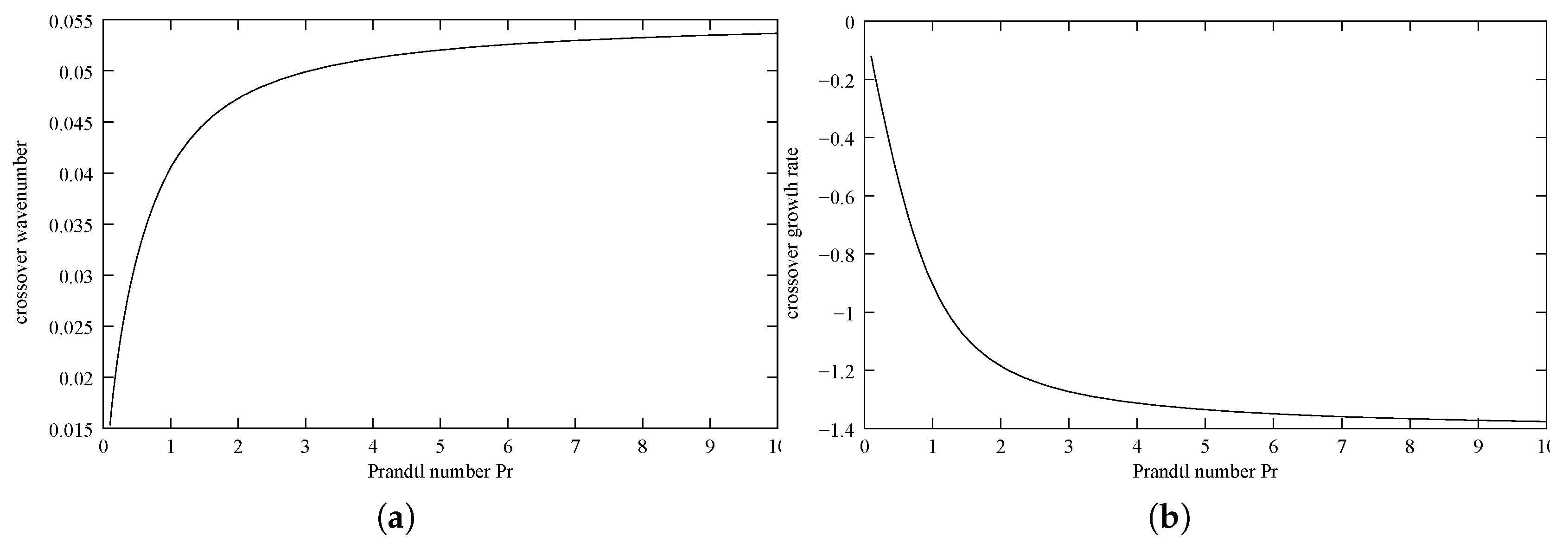
Identifying the critical surface in parameter space for the co-existence of the pair of intermediate wavenumber propagating modes and the long wave stationary modes (long wave thermal mode and long wave neutral temperature mode) is essential in mapping the parameter space. Continuation methods based on Newton iteration must search for either purely real (long wave stationary modes) or genuinely complex (intermediate wavenumber propagating modes). Figure 2 shows this critical curve and for four mode co-existence at fixed parametric values found by numerically solving for and simultaneously by Newton’s method. For it can be seen that the wavenumber of the crossover point is a decreasing function, whilst the growth rate is an increasing function. The four modes that co-exist along this critical curve are the two long wave stationary modes and two intermediate modes propagating from opposing directions. Figure 3 shows an analogous curve for the crossover point from stationary long waves to propagating steady intermediate waves. A Prandtl number of 1 is common for gases and a Prandtl number of 10 is common for liquids. The plots in Figure 3 show how the behavior of the fluids changes from a near gaseous state to a near liquid state.
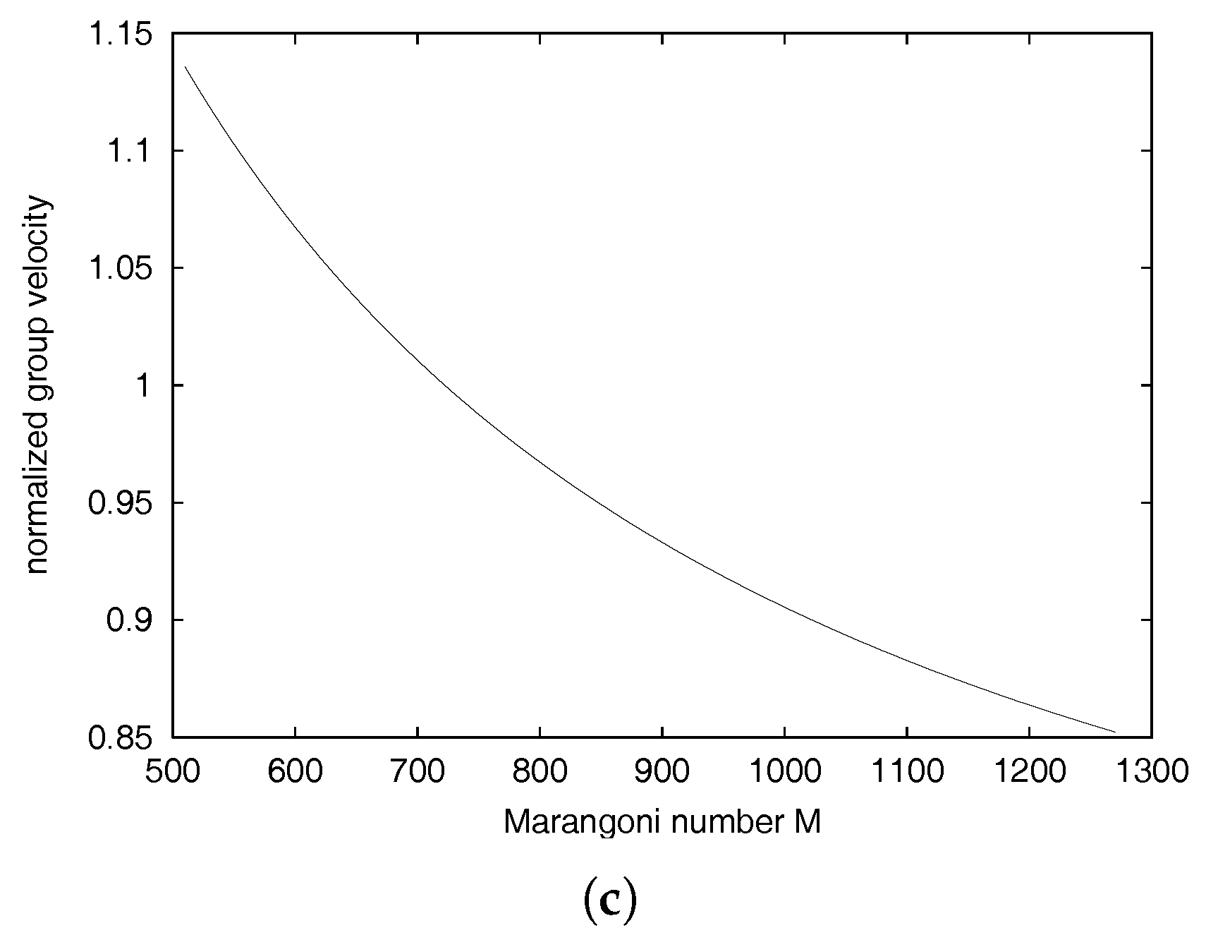
Once the critical surface dividing the wavenumber space into the two different regions of wave character has been identified, it is a simple matter to use parameter space continuation methods in k to find the remainder of the dispersion relation. Figure 4 summarizes the dispersion relation by plotting maximum growth rate and the wavenumber at which it is achieved for a given Marangoni number M at the values . There is jaggedness in the graph in Figure 4a as the wavenumber of maximum growth can switch modes. The normalized group velocity is also plotted as a function of the Marangoni number. It is clear that neutral stability is found by ramping up the Marangoni number to for the other parameters fixed at these values.
4.2. Critical Parameters via the Neutral Stability Method
Identifying the critical Marangoni number and associated wavenumber and frequency by continuation in k and M for fixed is computationally expensive if parameter space is to be mapped. Once a single critical parameter set is known, continuation along the neutral stability surface should be possible. Ref. [14] recognized that the Marangoni number only arises linearly in Equation (20), so that it is possible to solve the tangential stress boundary condition for M and eliminate all quantities , thus finding the neutral stability curve by the condition that at arbitrary k and with , is imposed by adjusting . Takashima [15] also used this technique. Neither study, however, identified the long wave stationary branches put forth here. The critical parameters are then found by minimizing M over k. In this paper, the relation was solved for M, and neutral stability was found by using Newton’s method to adjust s to achieve . Use of numerical root finding methods for s such that are faster than those that seek values of s such that .
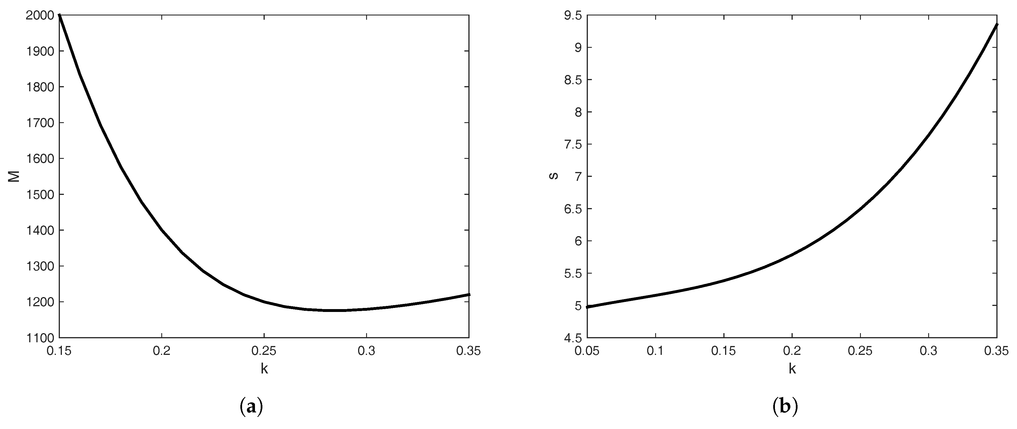
An algorithm for parameter space continuation in for by traversing the neutral stability surface was developed. The essential steps are to find the M-k and s-k neutral curves by computing a neighborhood in k surrounding an estimated critical point from adjacent values of . Subsequently, Newton’s method is used to find the minimum of the M-k neutral curve. This is illustrated in Figure 5 for the parameters , and . The crossover wavenumber neutral stability curve, i.e., that for which , is plotted, along with a curve showing the functional dependence of the frequency on the wavenumber k. A space of twenty values of each of was mapped by this method. Table 1 exhibits a sampling of the database built up from Newton continuation in . The range of parameters was selected to represent some physically realizable liquids (small capillary number and O(1) Prandtl number) and layer depths (microgravity to terrestrial gravity). From Table 1, it is clear that values of – are achievable under combinations of small capillary number and thin layers in liquids. Critical wavenumbers are typically of intermediate scale, neither long (<0.1, say) nor short (>10, say), but usually about .
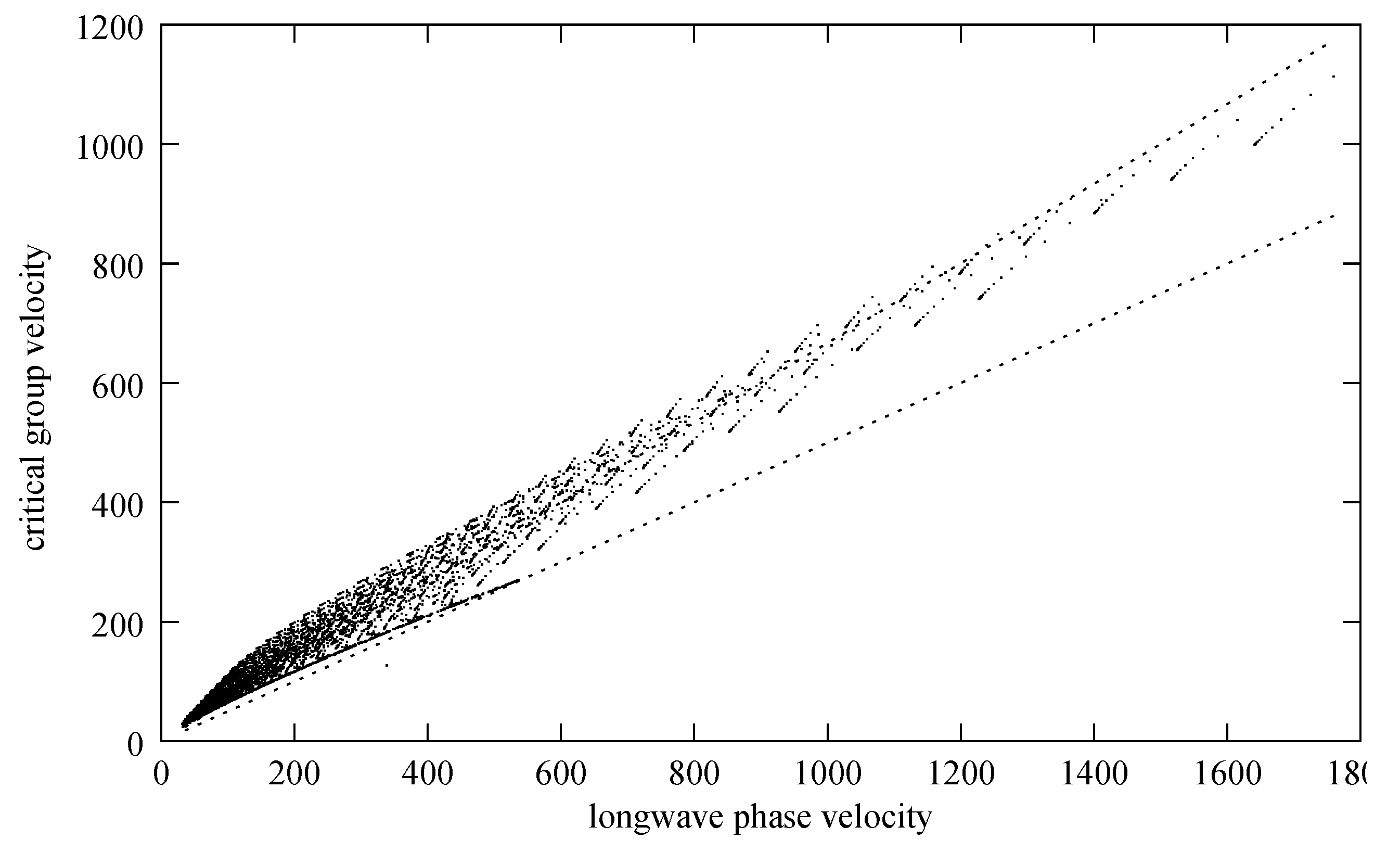
Figure 4 is suggestive that the group velocity of the critical mode might actually be well predicted by the long wave formula (20) for the phase velocity. The scatter plot in Figure 6 tests this hypothesis by crudely applying it to the entire mapped set of 8000 critical points. The critical group velocity, , is plotted against the longwave phase velocity, , for each of the 8000 critical parameter sets considered. The plot suggests that is the correct order of magnitude for the group velocity of the critical mode regardless of the parameter set in the range mapped. Furthermore, it is observed that the magnitude of the group velocity is constrained to be within to of the longwave phase velocity.
5. Conclusions
An analytical study based on linear theory has been presented that considers the development of instabilities that arise when a thin layer of a stably stratified fluid is heated from above for the Marangoni–Bénard problem. Particular focus was directed towards the value of the critical Marangoni number and to the influence of the lower boundary condition.
The stress-free model modifies the predicted critical Marangoni number to depend on the Galileo number (gravity effects), but reduces to under microgravity. It was not possible to find the cut-off wavenumber analytically as it requires solution of the dispersion relation to in small wavenumber k, but numerical solutions of the secular equation indicates, for all parameters tested, that < ∼0.05. This quantitative verification of the assumptions of KdV–KSV theory [8] under the stress-free boundary conditions leads one to conclude that any deficiencies of the theory must lie in the lower boundary condition. The analytic study of the long wave solutions to the secular equation for the no-slip model led to the surprising discovery that there are no infinitely long propagating modes. The three modes identified as are a neutral pure temperature mode, a damped viscous (pure velocity) mode, and a damped thermal (pure temperature) mode. The temperature and viscous modes both decay with increasing k, but the thermal mode increases in growth rate with small k. The prediction of an intersection point is computed by Newton continuation of the nonlinear solution of the secular equation. At the intersection of the two modes, the crossover point, there is co-existence of two propagating modes with the two stationary long modes. At higher wavenumbers, only the propagating modes exist. These modes are mapped by parameter space continuation in wavenumber, and a parametric study by continuation in the physical parameter space is made. Further developments in this research area could be facilitated by full numerical simulations.
Acknowledgments
This work was supported by funding from the Engineering and Physical Sciences Research Council (EPSRC) grant EP/I019790/1 on Microbubble cloud generation from fluidic oscillation: underpinning fluid dynamics. Funding was provided from the University of Sheffield for covering the costs to publish in open access.
Author Contributions
William B. Zimmerman and Julia M. Rees contributed equally to the theory and computation.
Conflicts of Interest
The authors declare no conflict of interest. The funding sponsors had no role in the design of the study; in the collection, analyses, or interpretation of data; in the writing of the manuscript, and in the decision to publish the results.
Abbreviations
The following abbreviations are used in this manuscript:
| KdV–KSV equation | Korteweg–de Vries–Kuramoto–Sivashinsky–Velarde equation |
| LST | Linear stability theory |
References
- Velarde, M.G.; Normand, C. Convection. Sci. Am. 1980, 243, 92–108. [Google Scholar]
- Sternling, C.V.; Scriven, L.E. Interfacial turbulence: Hydrodynamic instability and the Marangoni effect. Am. Inst. Chem. Eng. J. 1959, 5, 514–523. [Google Scholar] [CrossRef]
- Smith, K.A. On convective instability induced by surface-tension gradients. J. Fluid Mech. 1966, 24, 401–414. [Google Scholar] [CrossRef]
- Velarde, M.G.; Nepomnyashchy, A.A.; Hennenberg, M. Onset of oscillatory interfacial instability and wave motions in Bénard layers. Adv. Appl. Mech. 2001, 37, 167–238. [Google Scholar]
- MacInnes, J.M.; Pitt, M.J.; Priestman, G.H.; Allen, R.W.K. Analysis of two-phase contacting in a rotating spiral channel. Chem. Eng. Sci. 2012, 69, 304–315. [Google Scholar] [CrossRef]
- Linde, H.; Schwarz, E.; Groger, K. Zum aufreten des oszillatorishen regimes der Marangoni-instabilitat beim Stoffubergang. Chem. Eng. Sci. 1967, 22, 823–836. [Google Scholar] [CrossRef]
- Linde, H.; Chu, X.; Velarde, M.G. Oblique and head-on collisions of solitary waves in Marangoni–Bénard convection. Phys. Fluids 1993, 5, 1068–1070. [Google Scholar] [CrossRef]
- Nepomnyashchy, A.A.; Velarde, M.G. A three-dimensional description of solitary waves and their interaction in Marangoni-Benard layers. Phys. Fluids 1994, 6, 187–197. [Google Scholar] [CrossRef]
- Zimmerman, W.B.; Rees, J.M.; Hewakandamby, B.N. Numerical analysis of solutocapillary Marangoni-induced interfacial waves. Adv. Colloid Interface. Sci. 2007, 134–135, 346–359. [Google Scholar] [CrossRef] [PubMed]
- Rees, J.M.; Zimmerman, W.B. An intermediate wavelength, weakly nonlinear theory for the evolution of capillary gravity waves. Wave Motion 2011, 48, 707–716. [Google Scholar] [CrossRef]
- Davis, S.H.; Homsy, G.M. Energy stability theory for free-surface problems: Buoyancy-thermocapillary layers. J. Fluid Mech. 1980, 98, 527–553. [Google Scholar] [CrossRef]
- Lighthill, J. Waves in Fluids; Cambridge University Press: Cambridge, UK, 1978. [Google Scholar]
- Joseph, D.D.; Saut, J.C. Short-wave instabilities and ill-posed initial-value problems. Theor. Comput. Fluid Dyn. 1990, 1, 191–227. [Google Scholar] [CrossRef]
- Reichenbach, J.; Linde, H. Linear perturbation analysis of surface-tension-driven convection at a plane interface (Marangoni instability). J. Colloid Interface Sci. 1981, 84, 433–443. [Google Scholar] [CrossRef]
- Takashima, M. Surface tension driven instability in a horizontal liquid layer with a deformable free surface. II. Overstability. J. Phys. Soc. Jpn. 1981, 50, 2751–2756. [Google Scholar] [CrossRef]
Figure 1.
Growth rate vs. wavenumber k for , , , . The plot clearly illustrates an exponential growth of a long wave packet, subtended by and .
Figure 1.
Growth rate vs. wavenumber k for , , , . The plot clearly illustrates an exponential growth of a long wave packet, subtended by and .
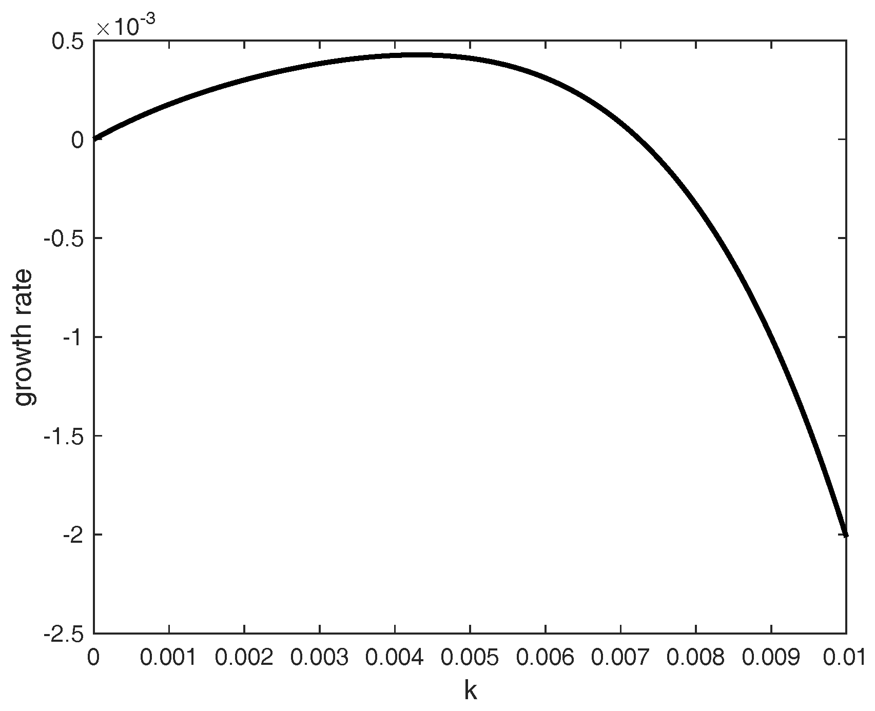
Figure 2.
Magnitude of velocity field on mm plane: (a) crossover wavenumber k; (b) growth rate ; for which and simultaneously at the parametric values , , and . Along this critical curve, four modes co-exist—the two long wave stationary modes and two opposite-directed intermediate propagating modes.
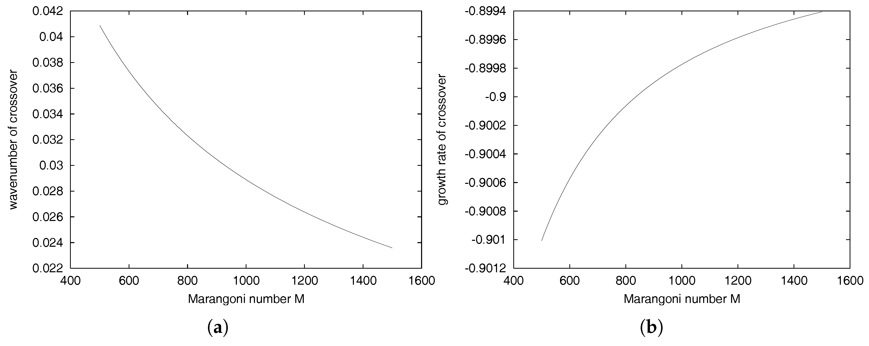
Figure 3.
Magnitude of velocity field on mm plane: (a) crossover wavenumber k; (b) growth rate ; for which and simultaneously at the parametric values and . Along this critical curve, four modes co-exist—the two long wave stationary modes and two opposite-directed intermediate propagating modes.
Figure 3.
Magnitude of velocity field on mm plane: (a) crossover wavenumber k; (b) growth rate ; for which and simultaneously at the parametric values and . Along this critical curve, four modes co-exist—the two long wave stationary modes and two opposite-directed intermediate propagating modes.

Figure 4.
(a) wavenumber ; (b) growth rate ; (c) group velocity reduced by long wave phase velocity (26) for which and for all k at the parametric values and . These curves identify the most dangerous mode (wavelength with most rapid growth or slowest decay). Clearly, there is neutral stability at . The jaggedness of (a) reflects the granularity of the discretization in k-M-continuation.
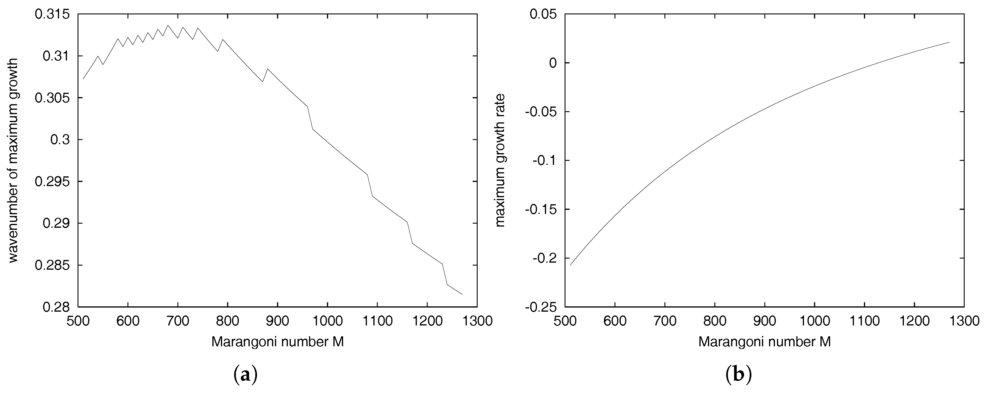

Figure 5.
Magnitude of velocity field on mm plane: (a) crossover wavenumber k for the M-k neutral stability curve () for the parameters . is found from the global minimum of the neutral curve and is the associated wavenumber; (b) frequency .
Figure 5.
Magnitude of velocity field on mm plane: (a) crossover wavenumber k for the M-k neutral stability curve () for the parameters . is found from the global minimum of the neutral curve and is the associated wavenumber; (b) frequency .

Figure 6.
Scatter plot of versus for the 8000 critical parameter sets mapped. This suggests that is the correct order of magnitude and a fair approximation for the group velocity of the critical mode regardless of the parameter set in the range mapped. Dotted lines have slope and .
Figure 6.
Scatter plot of versus for the 8000 critical parameter sets mapped. This suggests that is the correct order of magnitude and a fair approximation for the group velocity of the critical mode regardless of the parameter set in the range mapped. Dotted lines have slope and .


Table 1.
Critical values for fixed found by the neutral stability/minimization algorithm and parameter space continuation within the database. Samples were tested against the dispersion relation method and were found to be in agreement and global maximum of growth rate versus k. The table shows only selected values; the database is . There are twenty values for each parameter, spaced exponentially.
| K | Pr | G | |||
|---|---|---|---|---|---|
| 1.0 | 1.001 | 1.000 | 0.2820 | 6.664 | 1.032 |
| 1.0 | 1.001 | 1.833 | 0.2821 | 6.674 | 1.034 |
| 1.0 | 1.001 | 3.360 | 0.2823 | 6.692 | 1.036 |
| 1.0 | 1.001 | 6.160 | 0.2826 | 6.724 | 1.041 |
| 1.0 | 1.001 | 1.129 | 0.2833 | 6.783 | 1.049 |
| 1.0 | 1.001 | 2.069 | 0.2847 | 6.892 | 1.064 |
| 1.0 | 1.001 | 3.793 | 0.2877 | 7.095 | 1.087 |
| 1.0 | 1.001 | 6.952 | 0.2949 | 7.479 | 1.120 |
| 1.0 | 1.001 | 1.274 | 0.3140 | 8.264 | 1.152 |
| 1.0 | 1.001 | 2.336 | 0.3736 | 10.16 | 1.130 |
| 1.0 | 1.001 | 4.281 | 0.5052 | 14.17 | 1.008 |
| 1.0 | 1.001 | 7.848 | 0.5703 | 18.22 | 1.042 |
| 1.0 | 1.001 | 1.438 | 0.5501 | 21.89 | 1.334 |
| 1.0 | 1.001 | 2.637 | 0.4826 | 25.08 | 1.979 |
| 1.0 | 1.001 | 4.833 | 0.3936 | 27.34 | 3.224 |
| 1.0 | 1.001 | 8.859 | 0.3048 | 28.57 | 5.548 |
| 1.0 | 1.001 | 1.624 | 0.2296 | 29.13 | 9.835 |
| 1.0 | 1.001 | 2.976 | 0.1710 | 29.38 | 1.771 |
| 1.0 | 10. | 1.0 | 0.2105 | 210.3 | 1.693 |
| 8.859 | 10. | 1.0 | 0.2102 | 210.0 | 1.694 |
| 7.848 | 10. | 1.0 | 0.2069 | 207.4 | 1.702 |
| 1.0 | 10. | 1.0 | 0.1563 | 89.24 | 6.994 |
| 1.0 | 10. | 1.0 | 0.1403 | 156.2 | 2.096 |
© 2017 by the authors. Licensee MDPI, Basel, Switzerland. This article is an open access article distributed under the terms and conditions of the Creative Commons Attribution (CC BY) license (http://creativecommons.org/licenses/by/4.0/).
Share and Cite
MDPI and ACS Style
Zimmerman, W.B.; Rees, J.M. Excitation of Surface Waves Due to Thermocapillary Effects on a Stably Stratified Fluid Layer. Appl. Sci. 2017, 7, 392. https://doi.org/10.3390/app7040392
AMA Style
Zimmerman WB, Rees JM. Excitation of Surface Waves Due to Thermocapillary Effects on a Stably Stratified Fluid Layer. Applied Sciences. 2017; 7(4):392. https://doi.org/10.3390/app7040392
Chicago/Turabian StyleZimmerman, William B., and Julia M. Rees. 2017. "Excitation of Surface Waves Due to Thermocapillary Effects on a Stably Stratified Fluid Layer" Applied Sciences 7, no. 4: 392. https://doi.org/10.3390/app7040392
Note that from the first issue of 2016, this journal uses article numbers instead of page numbers. See further details here.