
Global and Continuous Pleasantness Estimation of the Soundscape Perceived during Walking Trips through Urban Environments

 , ,
, ,
Abstract
:1. Introduction
- The trend effect, which describes the fact that people often make predictions about the future based on trends that they have observed in the past, has been shown by Steffens & Guastavino, on a corpus of various 1-min length samples [29].
- A first experiment is based on different arrangements of two audio files, and aims to determine how the global temporal structure of a sound sequence affects its continuous and overall sound pleasantness appreciation. The sound sequences are built with the goal of assessing the effect of the temporal structure of the “background” sound environment. Therefore, strong markers of the soundscape or peaks in the sound levels were specifically avoided.
- A second experiment is based on the same principle, but with real sound sequences, played conjointly with video content, in order to investigate the same questions with natural sequences and a higher ecological validity.
2. Materials and Methods
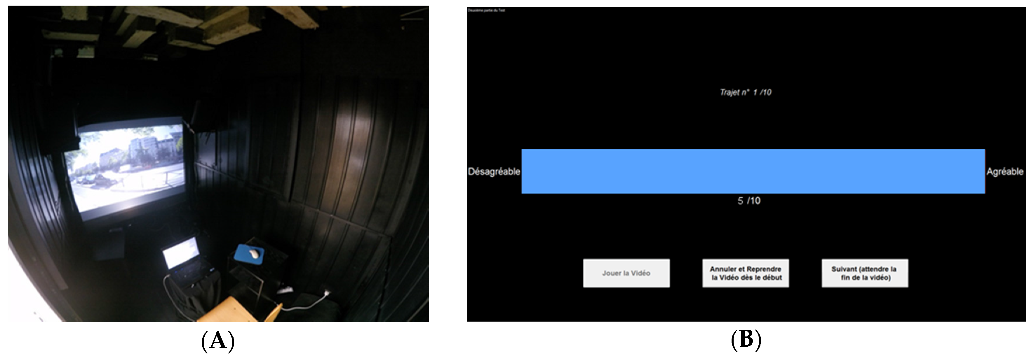
2.1. Apparatus
2.2. Procedure
2.3. Participants
2.4. Stimuli
2.4.1. First Experiment
2.4.2. Second Experiment
3. Results
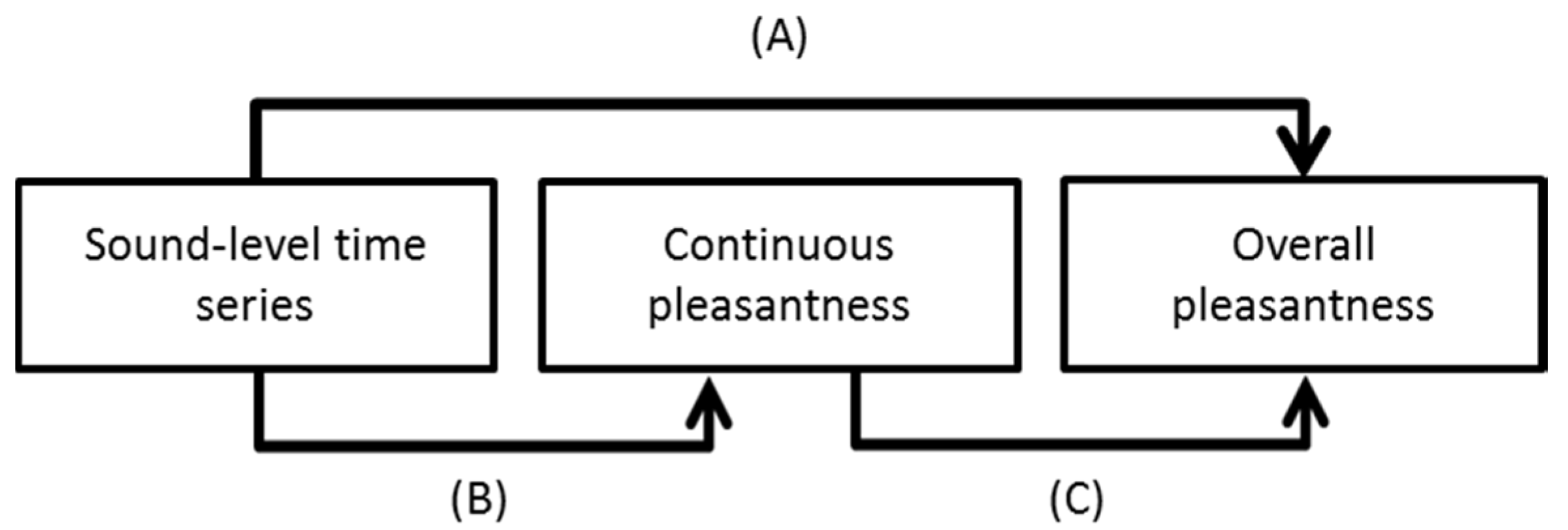
3.1. From Continuous to Global Perceived Pleasantness Assessment
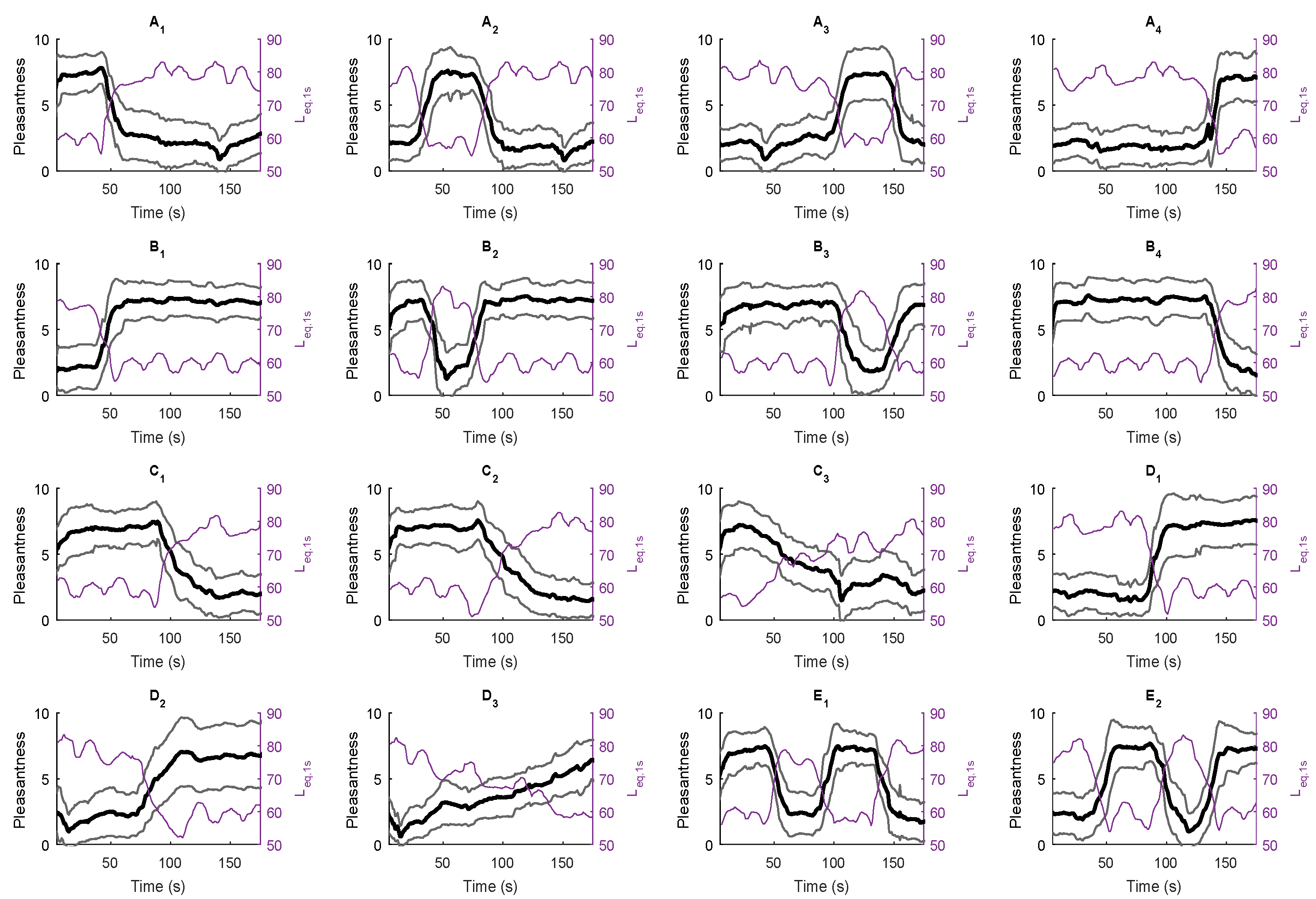
3.1.1. First Experiment
3.1.2. Second Experiment
3.2. From Measurements to Continuous and Retrospective Perceived Pleasantness
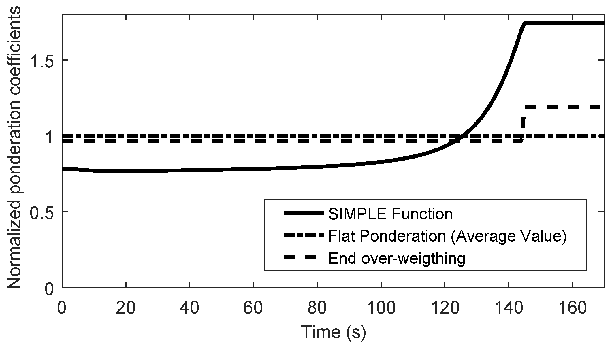
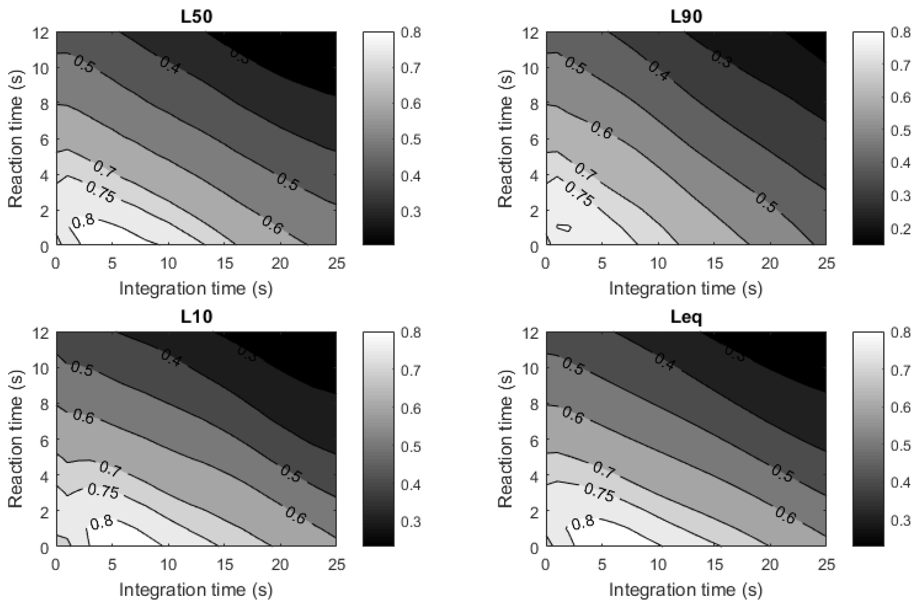
3.2.1. Continuous Sound Pleasantness Estimation Based on Noise Level Time Series
3.2.2. Global Sound Pleasantness Estimation Based on Sound Level Time Series
4. Discussion
- The sound sequences of the second experiment are less contrasted and more complex than the controlled sound sequences used in the first experiment. This attenuates the conclusions concerning a recency effect for the sound pleasantness assessment of real sound sequences. Moreover, as in the first experiment, the focus was to observe the influence of the temporal structure in an environment, so sound markers or events have been removed. Such events, as semantic content, are suspected to significantly influence the overall rating of the sound environment [43]. These events and markers, present in the second experiment, might have masked the recency and trend effects that were observed in the first experiment.
- The video content might have helped participants to analyze the sequences of the second experiment as a whole, thus attenuating the recency effect.
5. Conclusions
- The modeling of the recency effect, through the state-of-the-art SIMPLE model, improves the estimation of the global sound pleasantness over the controlled sound sequences. This effect tends to decline or disappear when the sound sequences are more realistic, including, among other things, some visual information.
- The global sound pleasantness can be estimated by using the median or the arithmetic average of the instantaneous sound pleasantness values.
- The instantaneous sound pleasantness is mainly impacted by the sound level during the last few seconds. Reaction and integration times are used by participants for estimating the continuous judgment of the pleasantness of the sound environment. The sound level time series can be more accurately taken into account with the SIMPLE model, which then highlights that the last 30 s also influence, although to a lesser extent, the instantaneous sound pleasantness assessments.
- Finally, the Global sound pleasantness can be accurately estimated based on the sound level time series of the 3 min sequences, either by relying on an intermediate estimation of the instantaneous sound pleasantness values, or directly based on the sound level time series, through an arithmetic average or a median value of the Leq,1s values. Both approaches are relevant, explaining about 60% of the variance in the global sound pleasantness, with an error inferior to 0.75 points over an 11-points scale.
Acknowledgments
Author Contributions
Conflicts of Interest
References
- Global Recommendations on Physical Activity for Health; World Health Organization: Geneva, Swizerland, 2010.
- Maurer Braun, L.; Read, A. The Benefits of Street-Scale Features for Walking and Biking; American Planning Association: Washington, DC, USA, 2015. [Google Scholar]
- Methorst, R.; Monterden i Bort, H.; Risser, R.; Sauter, D. Pedestrians’ Quality Needs. Final Report of the COST Project 358, Cheltenham: Walk21. Tight, M., Walker, J. Pedestrians’ Quality Needs Project, Posted 2010. Available online: http://www.walkeurope.org/final_report/default.asp (accessed on 4 Febuary 2017).
- King, E.A.; Murphy, E.; McNabola, A. Reducing pedestrian exposure to environmental pollutants: A combined noise exposure and air quality analysis approach. Transp. Res. D Transp. Environ. 2009, 14, 309–316. [Google Scholar] [CrossRef]
- Saelens, B.E.; Sallis, J.F.; Frank, L.D. Environmental correlates of walking and cycling: Findings from the transportation, urban design, and planning literatures. Ann. Behav. Med. 2003, 25, 80–91. [Google Scholar] [CrossRef] [PubMed]
- Ross, Z.; Kheirbek, I.; Clougherty, J.E.; Ito, K.; Matte, T.; Markowitz, S.; Eisl, H. Noise, air pollutants and traffic: Continuous measurement and correlation at a high-traffic location in New York City. Environ. Res. 2011, 111, 1054–1063. [Google Scholar] [CrossRef] [PubMed]
- Can, A.; Rademaker, M.; Van Renterghem, T.; Mishra, V.; Van Poppel, M.; Touhafi, A.; Theunis, J.; De Baets, B.; Botteldooren, D. Correlation analysis of noise and ultrafine particle counts in a street canyon. Sci. Total Environ. 2011, 409, 564–572. [Google Scholar] [CrossRef] [PubMed]
- Dekoninck, L.; Botteldooren, D.; Panis, L.I. An instantaneous spatiotemporal model to predict a bicyclist’s Black Carbon exposure based on mobile noise measurements. Atmos. Environ. 2013, 79, 623–631. [Google Scholar] [CrossRef]
- Guo, Z. Does the pedestrian environment affect the utility of walking? A case of path choice in downtown Boston. Transp. Res. D Transp. Environ. 2009, 14, 343–352. [Google Scholar] [CrossRef]
- Botteldooren, D.; Dekoninck, L.; Gillis, D. The influence of traffic noise on appreciation of the living quality of a neighborhood. Int. J. Environ. Res. Public Health 2011, 8, 777–798. [Google Scholar] [CrossRef] [PubMed]
- Davies, G.; Whyatt, J.D. A network-based approach for estimating pedestrian journey-time exposure to air pollution. Sci. Total Environ. 2014, 485, 62–70. [Google Scholar] [CrossRef] [PubMed]
- Lwin, K.K.; Murayama, Y. Modelling of urban green space walkability: Eco-friendly walk score calculator. Comput. Environ. Urban Syst. 2011, 35, 408–420. [Google Scholar] [CrossRef]
- Can, A.; Van Renterghem, T.; Botteldooren, D. Exploring the use of mobile sensors for noise and black carbon measurements in an urban environment. Acoustics 2012, 2012. [Google Scholar]
- Brocolini, L.; Lavandier, C.; Quoy, M.; Ribeiro, C. Measurements of acoustic environments for urban soundscapes: Choice of homogeneous periods, optimization of durations, and selection of indicators. J. Acoust. Soc. Am. 2013, 134, 813–821. [Google Scholar] [CrossRef] [PubMed]
- Liu, J.; Kang, J.; Luo, T.; Behm, H.; Coppack, T. Spatiotemporal variability of soundscapes in a multiple functional urban area. Landsc. Urban Plan. 2013, 115, 1–9. [Google Scholar] [CrossRef]
- Coensel, B.D.; Vanwetswinkel, S.; Botteldooren, D. Effects of natural sounds on the perception of road traffic noise. J. Acoust. Soc. Am. 2011, 129, EL148. [Google Scholar] [CrossRef] [PubMed]
- Lavandier, C.; Defréville, B. The contribution of sound source characteristics in the assessment of urban soundscapes. Acta Acust. United Acust. 2006, 92, 912–921. [Google Scholar]
- Ricciardi, P.; Delaitre, P.; Lavandier, C.; Torchia, F.; Aumond, P. Sound quality indicators for urban places in Paris cross-validated by Milan data. J. Acoust. Soc. Am. 2015, 138, 2337–2348. [Google Scholar] [CrossRef] [PubMed]
- Ishiyama, T.; Hashimoto, T. The impact of sound quality on annoyance caused by road traffic noise—An influence of frequency spectra on annoyance. JSAE Rev. 2000, 21, 225–230. [Google Scholar] [CrossRef]
- Berglund, B.; Hassmén, P.; Preis, A. Annoyance and Spectral Contrast Are Cues for Similarity and Preference of Sounds. J. Sound Vib. 2002, 250, 53–64. [Google Scholar] [CrossRef]
- Jeon, J.Y.; Lee, P.J.; Hong, J.Y.; Cabrera, D. Non-auditory factors affecting urban soundscape evaluation. J. Acoust. Soc. Am. 2011, 130, 3761–3770. [Google Scholar] [CrossRef] [PubMed]
- Jeon, J.Y.; Hong, J.Y.; Lee, P.J. Soundwalk approach to identify urban soundscapes individually. J. Acoust. Soc. Am. 2013, 134, 803–812. [Google Scholar] [CrossRef] [PubMed]
- Yu, L.; Kang, J. Factors influencing the sound preference in urban open spaces. Appl. Acoust. 2010, 71, 622–633. [Google Scholar] [CrossRef]
- Steele, D.; Guastavino, C. The role of activity in urban soundscape evaluation. In Proceedings of the Euronoise 2015, Maastricht, The Netherlands, 31 May–3 June 2015; pp. 1507–1512.
- Tarlao, C.; Steele, D.; Fernandez, P.; Guastavino, C. Comparing soundscape evaluations in French and English across three studies in Montreal. In Proceedings of the Inter-Noise 2016, Hamburg, Germany, 21–24 August 2016; pp. 21–24.
- Can, A.; Guillaume, G.; Gauvreau, B. Noise Indicators to Diagnose Urban Sound Environments at Multiple Spatial Scales. Acta Acust. United Acust. 2015, 101, 964–974. [Google Scholar] [CrossRef]
- Bennett, G.; King, E.; Curn, J.; Cahill, V.; Bustamante, F.; Rice, H. Environmental noise mapping using measurements in transit. In Proceedings of the ISMA 2010, Leuven, Belgium, 20–22 September 2010; pp. 1795–1809.
- De Coensel, B.; Sun, K.; Wei, W.; Van Renterghem, T.; Sineau, M.; Ribeiro, C.; Can, A.; Aumond, P.; Lavandier, C.; Botteldooren, D. Dynamic Noise Mapping based on Fixed and Mobile Sound Measurements. In Proceedings of Euronoise 2015, the 10th European Congress and Exposition on Noise Control Engineering, Maastricht, The Netherlands, 31 May–3 June 2015.
- Steffens, J.; Guastavino, C. Trend Effects in Momentary and Retrospective Soundscape Judgments. Acta Acust. United Acust. 2015, 101, 713–722. [Google Scholar] [CrossRef]
- Västfjäll, D. The “end effect” in retrospective sound quality evaluation. Acoust. Sci. Technol. 2004, 25, 170–172. [Google Scholar] [CrossRef]
- Susini, P.; McAdams, S.; Smith, B.K. Global and Continuous Loudness Estimation of Time-Varying Levels. Acta Acust. United Acust. 2002, 88, 536–548. [Google Scholar]
- Ponsot, E.; Verneil, A.-L.; Susini, P. Effect of sound duration on loudness estimates of increasing and decreasing intensity sounds. J. Acoust. Soc. Am. 2013, 134, 4063. [Google Scholar] [CrossRef]
- Fiebig, A.; Sottek, R. Contribution of Peak Events to Overall Loudness. Acta Acust. United Acust. 2015, 101, 1116–1129. [Google Scholar] [CrossRef]
- Luigi, M.; Massimiliano, M.; Aniello, P.; Gennaro, R.; Virginia, P.R. On the Validity of Immersive Virtual Reality as tool for multisensory evaluation of urban spaces. Energy Procedia 2015, 78, 471–476. [Google Scholar] [CrossRef]
- Maillard, J.; Kacem, A. Evaluation de la Qualité Acoustique des Parcours Piétonniers Urbains par Auralisation. In Proceedings of the CFA 2016, Le Mans, France, 11–15 April 2016.
- Aumond, P.; Can, A.; De Coensel, B.; Botteldooren, D.; Ribeiro, C.; Lavandier, C. Sound pleasantness evaluation of pedestrian walks in urban sound environments. In Proceedings of the ICA 2016, Buenos Aires, Argentina, 5–9 September 2016; p. 11.
- Kuwano, S.; Namba, S. Continuous judgment of level-fluctuating sounds and the relationship between overall loudness and instantaneous loudness. Psychol. Res. 1985, 47, 27–37. [Google Scholar] [CrossRef] [PubMed]
- Takeuchi, T.; Nelson, P.A. Optimal Source Distribution for Binaural Synthesis over Loudspeakers. J. Acoust. Soc. Am. 2002, 112, 2786. [Google Scholar] [CrossRef] [PubMed]
- Audiometric Classification of Hearing Impairements—BIAP Recommendation 02/1 Bis. Available online: http://www.biap.org/index.php?option=com_content&view=article&id=5%3Arecommandation-biap-021-bis&catid=65%3Act-2-classification-des-surdites&Itemid=19&lang=en (accessed on 19 December 2016).
- Le Bilan des Déplacements en 2014 à Paris; L’observatoire des Déplacements à Paris: Paris, France, 2014.
- Brown, G.D.A.; Neath, I.; Chater, N. A temporal ratio model of memory. Psychol. Rev. 2007, 114, 539–576. [Google Scholar] [CrossRef] [PubMed]
- Brown, G.D.A. HomePage: Brown, Gordon D.A. Available online: http://homepages.warwick.ac.uk/staff/G.D.A.Brown/simple/ (accessed on 19 Junuary 2016).
- Fan, J.; Thorogood, M.; Pasquier, P. Automatic Soundscape Affect Recognition Using A Dimensional Approach. J. Audio Eng. Soc. 2016, 64, 646–653. [Google Scholar] [CrossRef]
- Viollon, S.; Lavandier, C.; Drake, C. Influence of visual setting on sound ratings in an urban environment. Appl. Acoust. 2002, 63, 493–511. [Google Scholar] [CrossRef]
- Gille, L.-A.; Marquis-Favre, C.; Weber, R. Noise sensitivity and loudness derivative index for urban road traffic noise annoyance computation. J. Acoust. Soc. Am. 2016, 140, 4307. [Google Scholar] [CrossRef] [PubMed]


| Street Name | Description | Labels |
|---|---|---|
| Rue de Tolbiac | Large street | T |
| Passage Vendrezanne | Pedestrian Street | V |
| Avenue Blanqui | Avenue | Bl |
| Jardin Brassaï | Park | Br |
| Avenue Italie | Large Avenue | I |
| Rue des 2 avenues | Pedestrian street | D |
| Parc de Choisy | Park | ChP |
| Rue du Moulinet | Street | M |
| Avenue Choisy | Large Street | ChA |
| Sequences | L50 (L10 − L90) | Pmean | GP | ΔGP-Pmean | Sequences | L50 (L10 − L90) | Pmean | GP | ΔGP-Pmean |
|---|---|---|---|---|---|---|---|---|---|
| A1[αβββ fast] | 76 (24) | 3.7 (2.3) | 2.9 (1.9) | −0.7 | C1[ββαα fast] | 65 (23) | 4.9 (1.9) | 4.2 (1.9) | −0.7 |
| A2[βαββ fast] | 76 (25) | 3.5 (2.3) | 2.6 (1.2) | −0.9 | C2[ββαα medium] | 63 (25) | 4.8 (2.2) | 4.3 (1.7) | −0.5 |
| A3[ββαβ fast] | 76 (24) | 3.6 (2.1) | 3.4 (1.7) | −0.2 | C3[ββαα slow] | 70 (21) | 4.2 (2.3) | 3.5 (1.8) | −0.7 |
| A4[βββα fast] | 76 (24) | 2.9 (2.0) | 3.4 (1.4) | 0.5 | D1[ααββ fast] | 64 (26) | 4.5 (2.4) | 4.9 (1.6) | 0.4 |
| B1[βααα fast] | 60 (22) | 5.9 (2.1) | 6.4 (1.5) | 0.6 | D2[ααββ medium] | 63 (25) | 4.5 (1.7) | 5.5 (1.6) | 1.0 |
| B2[αβαα fast] | 60 (22) | 6.0 (2.1) | 6.3 (1.4) | 0.3 | D3[ααββ slow] | 68 (20) | 3.6 (2.2) | 4.1 (1.6) | 0.5 |
| B3[ααβα fast] | 60 (22) | 5.6 (1.9) | 5.7 (2.2) | 0.1 | E1[βαβα fast] | 62 (24) | 5.0 (2.6) | 4.8 (1.9) | −0.2 |
| B4[αααβ fast] | 60 (23) | 6.3 (1.8) | 5.7 (1.9) | −0.6 | E2[αβαβ fast] | 63 (25) | 4.8 (2.2) | 5.1 (2.0) | 0.3 |
| Presumed Factors | Variables | Code |
|---|---|---|
| Mean value | Mean value | Pmean |
| Trend effect | Standarized coefficient of the time regression calculations as proposed in [29] | Ptrend |
| Recency effect | Rate averaged over the last 30 s | Pend |
| Primacy effect | Rate averaged over the first 30 s | Pstart |
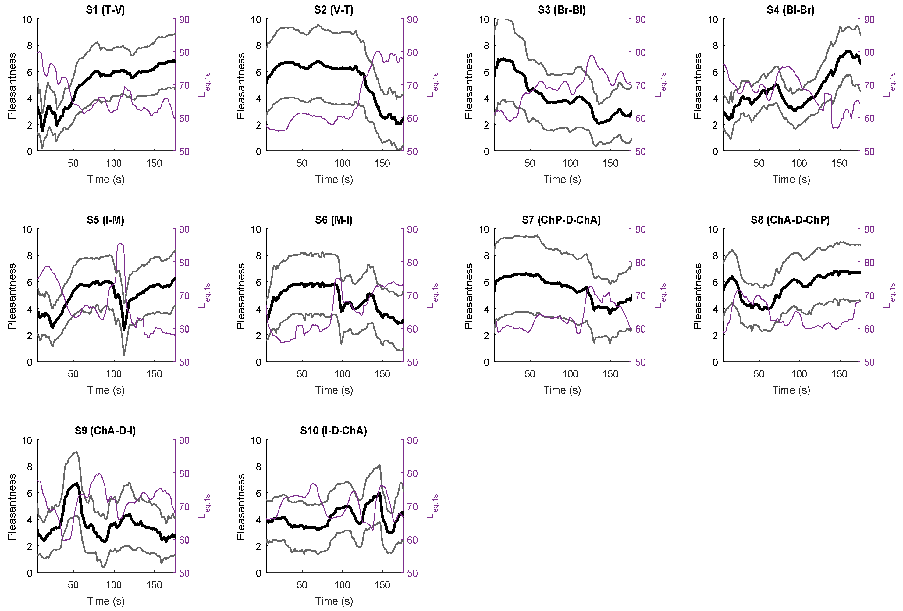
| Sequence Number | Ordered Characteristic Points | L50 (L10 − L90)—dB | Pmean | GP | ΔGP-Pmean |
|---|---|---|---|---|---|
| S1 | T-V | 64 (13) | 5.1 | 6.1 | 1 |
| S2 | V-T | 61 (22) | 5.3 | 6.6 | 1.3 |
| S3 | Br-Bl | 69 (16) | 4.1 | 4.6 | 0.5 |
| S4 | Bl-Br | 68 (17) | 4.6 | 5.6 | 0.9 |
| S5 | I-M | 65 (19) | 5.0 | 5.9 | 0.9 |
| S6 | M-I | 64 (17) | 4.7 | 4.5 | −0.1 |
| S7 | ChP-D-ChA | 62 (11) | 5.5 | 7.5 | 2.0 |
| S8 | ChA-D-ChP | 62 (11) | 5.7 | 6.8 | 1.0 |
| S9 | ChA-D-I | 72 (16) | 3.6 | 4.7 | 1.0 |
| S10 | I-D-ChA | 69 (11) | 4.1 | 4.0 | −0.1 |
| Equations | Explained Variance | R2, F, p, and RMSE Values |
|---|---|---|
| 21.5 − 0.24L50 | 58% | R2 = 0.63, F(2,8) = 13.4, p < 0.01, RMSE = 0.58 |
| 27.8 − 0.33Lmean | 54% | R2 = 0.59, F(2,8) = 11.6, p < 0.01, RMSE = 0.77 |
| 18.6 − 0.18Leq | 15% | R2 = 0.25, F(2,8) = 2.53, p = 0.15, RMSE = 1.06 |
© 2017 by the authors. Licensee MDPI, Basel, Switzerland. This article is an open access article distributed under the terms and conditions of the Creative Commons Attribution (CC BY) license ( http://creativecommons.org/licenses/by/4.0/).
Share and Cite
Aumond, P.; Can, A.; De Coensel, B.; Ribeiro, C.; Botteldooren, D.; Lavandier, C. Global and Continuous Pleasantness Estimation of the Soundscape Perceived during Walking Trips through Urban Environments. Appl. Sci. 2017, 7, 144. https://doi.org/10.3390/app7020144
Aumond P, Can A, De Coensel B, Ribeiro C, Botteldooren D, Lavandier C. Global and Continuous Pleasantness Estimation of the Soundscape Perceived during Walking Trips through Urban Environments. Applied Sciences. 2017; 7(2):144. https://doi.org/10.3390/app7020144
Chicago/Turabian StyleAumond, Pierre, Arnaud Can, Bert De Coensel, Carlos Ribeiro, Dick Botteldooren, and Catherine Lavandier. 2017. "Global and Continuous Pleasantness Estimation of the Soundscape Perceived during Walking Trips through Urban Environments" Applied Sciences 7, no. 2: 144. https://doi.org/10.3390/app7020144
APA StyleAumond, P., Can, A., De Coensel, B., Ribeiro, C., Botteldooren, D., & Lavandier, C. (2017). Global and Continuous Pleasantness Estimation of the Soundscape Perceived during Walking Trips through Urban Environments. Applied Sciences, 7(2), 144. https://doi.org/10.3390/app7020144