Imaging Flow Velocimetry with Laser Mie Scattering


Bremen Institute for Metrology, Automation and Quality Science (BIMAQ), University of Bremen, Linzer Str. 13, 28359 Bremen, Germany
Appl. Sci. 2017, 7(12), 1298; https://doi.org/10.3390/app7121298
Submission received: 9 November 2017
/
Revised: 6 December 2017
/
Accepted: 7 December 2017
/
Published: 13 December 2017
(This article belongs to the Special Issue Optics and Spectroscopy for Fluid Characterization)
Abstract
:Imaging flow velocity measurements are essential for the investigation of unsteady complex flow phenomena, e.g., in turbomachines, injectors and combustors. The direct optical measurement on fluid molecules is possible with laser Rayleigh scattering and the Doppler effect. However, the small scattering cross-section results in a low signal to noise ratio, which hinders time-resolved measurements of the flow field. For this reason, the signal to noise ratio is increased by using laser Mie scattering on micrometer-sized particles that follow the flow with negligible slip. Finally, the ongoing development of powerful lasers and fast, sensitive cameras has boosted the performance of several imaging methods for flow velocimetry. The article describes the different flow measurement principles, as well as the fundamental physical measurement limits. Furthermore, the evolution to an imaging technique is outlined for each measurement principle by reviewing recent advances and applications. As a result, the progress, the challenges and the perspectives for high-speed imaging flow velocimetry are considered.
1. Introduction
Understanding, designing and optimizing flows is crucial, e.g., for improving fuel injections [1], combustions [2,3], fuel cells [4], wind turbines [5], turbomachines [6], human air and blood flows in medicine [7,8], as well as for the fundamental task of modeling flow turbulence [9]. For this purpose, optical measurement methods are essential tools that promise fast and precise field measurements of complex flows.
The advances of optoelectronic components and systems, in particular concerning powerful pulsed lasers (up to 1 J/pulse) with up to megahertz repetition rate and high-speed cameras with megapixel image resolution, allow qualitative flow imaging with ultra-high speed, up to 1 MHz [10]. The combination of powerful lasers and high-speed cameras enables the fast imaging of two or three flow dimensions. Note, however, that at the maximum megahertz acquisition rate, the available number of successive laser pulses is limited to about 100 pulses. Besides a qualitative understanding of complex flow phenomena, the flow field needs to be quantified. An essential physical quantity for understanding the flow behavior is the flow velocity, which is the sole measurand that is considered in the subsequent article.
In order to optically measure the flow velocity, the flow of interest is illuminated. For this purpose, a laser light source is usually applied, because laser light sources provide a high light power and a narrow linewidth. Both are beneficial for reducing the cross-talk between the optical measurement and the ambient light. The incident light is scattered on the fluid molecules or atoms, and the scattered light is detected and analyzed. As the size of the fluid atoms or molecules in the order of 0.1 nm is significantly smaller than the wavelength of visible light (0.4 μm–0.8 μm), the light scattering is so-called Rayleigh scattering. Optical flow velocity measurements based on Rayleigh scattering are described for instance in [11,12,13,14,15,16,17]. An overview article exists from Miles, 2001 [18]. The flow velocity measurements are based on the optical Doppler effect, which causes a shift in the observed scattered light frequency due to the scattering at the moving fluid particles. The evaluated Doppler frequency is proportional to the flow velocity in the inertial frame of the measurement system.
Rayleigh scattering has a comparatively low scattering efficiency, which means that the ratio between the scattered light intensity and the incident is low. For this reason, a temporal averaging in the order of 16 min is required to achieve an acceptable measurement uncertainty of 2% for the flow velocity images of a tube flow with a maximum velocity of 120 m/s [19,20]. Faster flow velocity measurements are possible for single point measurements. A single point measurement system with 32 kHz [21] was reported, as well as a 10 kHz measurement system with a minimal accuracy of 1.23 m/s [22]. Hence, the fast measurement of flow velocity images with kilohertz rates and a low uncertainty is only achievable by increasing the scattering efficiency of the scattering particles.
Increasing the scattering efficiency can be achieved by inserting scattering particles (if not naturally present), which follow the flow with negligible slip and do not disturb the flow. The insertion of particles is called seeding, and the particles are seeding particles. In the Rayleigh scattering regime, the scattering efficiency is proportional to the particle diameter to the power of four. Hence, doubling the particle diameter results in a 16-times higher scattering efficiency. This condition changes in the Mie scattering regime [23,24,25], i.e., when the particle size is near the wavelength of the light. As a compromise between a high scattering efficiency and a negligible slip, typical seeding particles have a size between 100 nm and several micrometer [26]. Hence, the use of seeding particles leads to optical flow measurements based on Mie scattering. While Rayleigh scattering is an elastic light scattering, which allows one to measure the velocity, the pressure and the temperature of the fluid [19,20], Mie scattering is an elastic light scattering that only allows one to measure the particle velocity. However, the scattering efficiency is increased by several orders of magnitude, which enables the measurement of flow velocity images with a lower measurement uncertainty at an identical spatial and temporal resolution with the same laser power. The other way around, the higher scattering intensity also allows a higher spatiotemporal resolution, image size and measurement rate at an identical measurement uncertainty with the same laser power. For this reason, the article is focused on optical flow velocity measurement techniques based on Mie scattering, which typically require seeding.
A large variety of different measurement techniques based on Mie scattering exists. In particular concerning the improved scattered light energy, one fundamental question is the existence and the magnitude of physical measurement limits, which hold for any measurement technique. Understanding these limits allows one to identify the potential for the future development of each measurement technique. Furthermore, the existence of a possibly superior technique needs to be clarified. Such a unified broad consideration of the different flow velocity measurement techniques based on Mie scattering, starting with a physical categorization of the different techniques, is missing.
For this reason, the aim of the article is to summarize and to review the developments, recent advances and fundamental limits of the different imaging flow velocity measurement principles based on Mie scattering. At first, the physical measurement principles are explained in Section 2. Next, the development towards an imaging technique is described for each principle in Section 3. Thereby, it is focused on the development of high-speed imaging measurement systems. Research results regarding fundamental limits of the measurement techniques are then presented in Section 4. Finally, application examples, as well as the respective challenges and perspectives are discussed in Section 5. Note that the focus is set on measurement techniques for meso-scale flow applications with dimensions between millimeter and meter. A current review of micro-scale flow metrology can be found in [27]. However, the present review is not regarding certain flow applications, but the development of the different flow measurement techniques and their fundamental measurement limits.
2. Measurement Approaches
2.1. Application of Mie Scattering
In order to obtain Mie scattering, the measurement approaches require scattering particles in the flow to be measured. If no natural scattering particles exist, artificial particles are added to the flow, which is known as seeding. The generation, the characterization and the application of different seeding particles is described in [26]. As an example, a typical liquid seeding material for flows with ambient temperature is diethylhexyl sebacate (DEHS), and a typical solid seeding material for flame flows is titanium dioxide (TiO). Due to the typically necessary seeding, the flow measurement approaches based on Mie scattering are intrusive techniques.
Since the light that is scattered on the particles is detected and evaluated, the velocity of the particle motion is measured. Note that it is a common case that the desired quantity is not the particle velocity. However, the particle velocity equals the flow velocity, if the particles follow the flow with no slip, if the particles have no self-motion and if the inserted particles do not change the flow behavior. For the derivation of the different measurement approaches, these ideal conditions are assumed to be fulfilled. The otherwise resulting limits of measurability are treated in Section 4.
The drawbacks of using seeding particles to achieve Mie scattering are accepted due to the advantage of a significantly increased scattered light intensity in comparison with flow velocity measurements based on Rayleigh scattering with no seeding particles. In order to quantify the improvement of the scattered light intensity, the calculated scattering cross-section is shown in Figure 1 as a function of the radius of a scattering particle that is assumed to be spherical and made of DEHS. The calculation is conducted according to [25] for a refractive index of 1.45, which is valid for DEHS at a light wavelength of 650 nm. In the Rayleigh scattering regime, the scattering cross-section increases proportional to the sixth power of the particle radius. For an increased scattering particle size from 0.1 nm (order of magnitude of a molecule, Rayleigh scattering) to 1 μm (typical order of magnitude of a seeding particle, Mie scattering), the scattering cross-section is increased by more than 16 orders of magnitude. Considering a spatial resolution of 100 μm3 with air at normal pressure and room temperature as fluid, about fluid molecules are present according to the ideal gas law. Hence, the advantage of the higher scattering cross-section of seeding particles is partially equalized by the low number of scatterers. As a result, an increase of the scattering power of 1000 remains for the considered example. Another beneficial aspect of using seeding particles is the reduced light extinction, because the seeding is usually applied locally. Furthermore, the angular-dependent scattering and polarization effects have to be taken into account. For instance, Mie scattering has in general a stronger forward scattering than sidewards and backward scattering, which means a reduced light extinction in comparison to Rayleigh scattering. As a result, the potential of Mie scattering approaches for imaging flow measurements with acceptable uncertainty also at high measurement rates is illustrated, in particular with respect to the necessary distribution of the available light energy over space and time.
2.2. Scattered Light Evaluation
The velocity measurement approaches differ in the type of evaluation of the detected scattered light. One approach is to make use of the optical Doppler effect and to evaluate the momentum of the scattered light photons. Note that the photon momentum is Planck’s constant divided by the wavelength, so that the photon momentum also represents the wavelength property or the energy of a photon. The second approach follows from the kinematic definition of the velocity and the evaluation of the position property of the scattered light photons. Hence, the developed measurement principles can be categorized into two groups [28]:
- Doppler principles,
- Time-of-flight principles.
The Doppler principles are based on the optical Doppler effect that occurs for light scattering at a moving object. In this fashion, the frequency shift (Doppler frequency) of the light scattered on a single particle (or multiple particles) is measured, and the Doppler frequency depends on the particle velocity. The relation between the particle velocity and the Doppler frequency reads: [29,30]
where denotes the wavelength of the incident light and is the measured velocity component along the bisecting line of the angle between the light incidence direction from the illumination source and the observation direction of the scattered light, cf. Figure 2. Note that the relation is an approximate solution for particle velocities significantly smaller than the light velocity, which applies for the flows considered here. As a result, a single velocity component is obtained with the given measurement configuration, and the vector is the sensitivity vector. The measurement of all three velocity components requires three measurements with different incidence or different observation directions, so that the three sensitivity vectors span a three-dimensional space. Note further that Equation (1) is an approximate solution for velocities significantly smaller than the light velocity, which is applicable for the considered flows here. The remaining task is to determine the Doppler frequency of the scattered light signal, where the different measurement principles can be subdivided into Doppler principles with amplitude-based and frequency-based signal evaluation procedures.
The Doppler principles with an amplitude-based signal evaluation make use of the spectral transmission behavior of an optical filter. The optical filter converts the frequency information of the scattered light into an intensity information, which is finally measurable with a photodetector or camera. As the optical filter, an atomic or molecular filter or an interferometric filter is used. The interferometer can be a two-ray or a multiple ray interferometer. Note that the use of a filter requires laser light illumination with a significantly smaller linewidth than the linewidth of the filter transmission curve. Otherwise, the transmission curve of the filter is not resolved.
The Doppler principles with frequency-based signal evaluation also use interferometry. However, the scattered light is not superposed with itself, but with light with a different frequency. If the superposed light has no velocity-dependent shift in frequency, the measurement method is called a reference method. The superposed light is, e.g., from the illumination light source or a frequency comb. If the superposed light is also scattered light, but with a different Doppler frequency shift due to a different light incidence or observation direction, the difference of both Doppler frequencies is evaluated, and then, the measurement method is called the difference method.
The time-of-flight principles are based on the kinematic velocity definition, which reads for one velocity component:
with as the change in space during the time period . The approximation in Equation (2) is valid when the particle acceleration during the measurement is negligible. This is a common assumption, which reduces the required number of pairs of position and time to two, cf. Figure 3. Either the change of the particle position for a given time period or the time period for a given spatial distance is then measured. Accordingly, the time-of-flight principles can be subdivided into two categories using time measurements or space measurements. Instead of two pairs of position and time, also a higher number of pairs can be acquired to take the acceleration into account where necessary [31,32,33]. Furthermore, the time-of-flight principles are also capable of performing three component measurements, e.g., with planar illumination, planar detection and at least two observation directions for triangulation.
An overview of the proposed categorization of the different measurement approaches is shown in Figure 4. Referring to the “16th International Symposium on Applications of Laser Techniques to Fluid Mechanics” in the year 2012, 79% of the 220 contributions contain or concern flow velocity measurements. An amount of 90% of these contributions is related to time-of-flight principles, while 10% is related to Doppler principles. For the articles concerning time-of-flight measurement principles, a majority of 99% considers or applies space measurement methods. This strong focus on space measuring time-of-flight principles is due to the commercial availability of respective measurement systems that are capable of simultaneously acquiring up to three components of three-dimensional velocity fields. As a result, these systems are widely applied, and the related research work is reported. In contrast to this, measurement systems based on other principles currently seem to have a lag in development. However, in particular, Doppler principles are widely used as well and are advantageous for certain applications, which are illustrated for two examples. With a perpendicular arrangement of the illumination and observation direction, Doppler and time-of-flight principles allow one to measure different velocity components. For narrow optical accesses, which means low numerical apertures, the measurement of all three velocity components with a single principle is only achievable with additional observation or light incidence directions. If the additional optical access is not available or undesired, then the combination of both principles allows one to obtain measurements of all three velocity components with only one light incidence direction and one observation direction [34,35,36]. A further example of a beneficial combination of Doppler and time-of-flight principles is reported in [37], where a time-of-flight principle is used to resolve the velocity field image, but with a lower spatial and temporal resolution than the simultaneous single point Doppler measurement. As a result, turbulence investigations in an unsteady swirl flow could be performed together with an analysis of the global flow structures. The two examples show that hybrid approaches of combining Doppler and time-of-flight principles are possible and can offer advantages. The examples further demonstrate that each of the two fundamental measurement approaches has its own characteristics and benefits and that both approaches complement each other. In a physical sense, both approaches are complementary by evaluating the photon momentum or position.
3. Developed Measurement Techniques and Their Imaging Evolution
3.1. Fundamentals for the Evaluation of the Measurement Techniques
The quantity of interest is the fluid velocity (or flow velocity):
which is in general a time-dependent vector field in the three-dimensional space with as the space vector and t as the time variable. Hence, the flow measurements can be characterized and evaluated based on the following properties:
- The flow velocity is a vector quantity. Therefore, the number of measured velocity components is an important property. The abbreviated form 1c, 2c or 3c means that one, two or three components are measured, respectively.
- In order to characterize the spatial behavior of the flow velocity, the number of resolved space dimensions is an important property. Measurements are for instance pointwise, along a line, planar or volumetric, which is indicated by the abbreviated forms 0d, 1d, 2d or 3d, respectively. Characterizing the measurement along each space dimension is possible with the following parameters (cf. Figure 5a):
- -
- spatial resolution,
- -
- spatial distance between the adjacent measurements,
- -
- number of measurements along the respective space dimension or size of the measurement volume in the respective space dimension.
- In addition, the temporal behavior of the measured flow velocity is characterized with the parameters
- -
- temporal resolution,
- -
- temporal distance between the sequent measurements or measurement rate,
- -
- number of measurements along the time dimension or measurement duration.
The term measurement rate requires temporally-equidistant measurements. Otherwise, a mean measurement rate can be specified. The introduced terms are explained in Figure 5b. Note that the temporal resolution does not necessarily equal (or is smaller than) the reciprocal value of the measurement rate. Both quantities are independent. - Each velocity value over space and time can finally be characterized with a measurement uncertainty by applying the international guide to the expression of uncertainty in measurements (GUM) [38,39]. According to the GUM, the measurement uncertainty is a parameter, associated with the result of a measurement, that characterizes the dispersion of the values that could reasonably be attributed to the measurand.
- Due to possible cross-sensitivities (for instance with respect to the temperature, vibrations or electromagnetic fields) or other impairments of the measurements (for instance limited optical access), it is important if the measurements concern non-reactive or reactive flows (flames), if the measurements are performed in a laboratory or in an industrial environment, if the measurement object is a simplified model or the real measurement object. For this reason, the surrounding and boundary conditions have to be described.
In the following subsection, the development of each measurement approach from Section 2 to an imaging flow velocimetry system is summarized. Note that the summary is not meant to be exhaustive, but to give an overview of the state-of-the-art of current flow measurement systems. Since it is focused on the development of the respective measurement systems for achieving at least 2d1c measurements with high speeds, application examples, as well as the discussion of the measurement uncertainty are outsourced to Section 5.
3.2. Measurement Techniques Using the Doppler Principle
3.2.1. Amplitude-Based Signal Evaluation
In 1970, Jackson and Paul described a 0d reference laser Doppler velocimeter, where the scattered light with the Doppler frequency shift is analyzed with a confocal piezo-electrically-scanned Fabry–Pérot interferometer (FPI) [40]. The position of the maximal transmitted light signal through the FPI is a measure of the flow velocity. For 2d measurements, an FPI with planar mirrors can be used. Examples for such measurements are reported for Rayleigh scattering [12] and the fluid motion of the self-glowing Sun [41]. In 2013, Büttner et al. presented 1d flow measurements based on Mie scattering, but only for seven pixels [42]. The imaging to the FPI is performed with a self-made fiber-bundle with seven multi-mode fibers. For planar Doppler velocimetry with FPI (FPI-PDV), the crucial challenge is to achieve a high effective finesse of the interferometer. The finesse degrades with an increasing numerical aperture, which is required for maximizing the signal to noise ratio and for realizing an acceptable working distance. One solution to decouple the uncertainty between the FPI resolution and the numerical aperture was presented in 2003 by using single-mode fibers with an integrated FPI based on fiber Bragg grating technology [43]. A challenge for achieving a high signal to noise ratio is the low acceptance angle of single-mode fibers compared with multi-mode fibers. The fiber-integrated FPI approach was tested for 0d measurements on a rotating disc. The development of an FPI-PDV system for 2d flow measurements is an open task.
In place of a multiple ray interferometer, a two-ray interferometer can also be used, which is easier to apply for 2d measurements. In 1978, Smeets and George described a 0d reference laser Doppler velocimeter with a Michelson interferometer (MI) [44,45]. The extension to planar Doppler velocimetry with MI (MI-PDV) followed in 1982 by Oertel, Seiler and George [46,47], who named the measurement approach Doppler picture velocimetry (DPV). The mirror in the reference path of the interferometer is slightly tilted to generate a linear changing optical path difference and, thus, parallel interference fringes over the image. The velocity-dependent phase shift of these fringes is then determined with an image processing. The developed DPV system consists of a cwargon ion laser emitting at 514.5 nm and a charge coupled device (CCD) camera with 1374 × 1024 pixels and a shutter time of 2 ms [48]. An image series was not acquired, but CCD cameras usually provide a maximal frame rate of <60 Hz. In order to increase the sensitivity of the MI, a dispersive element (iodine vapor cell) was inserted in the reference path by Landolt and Rösgen in 2009 [49,50]. Furthermore, a normal CCD and an intensified CCD camera with an image resolution of 1008 × 1008 and 1280 × 1024 pixels are applied, respectively. The light sheets are generated with a pulsed Nd:YAG laser emitting at 532 nm with 100 mJ/pulse and a pulse width of 40 ns. The pulse repetition rate amounts to 10 Hz. High-speed flow imaging with MI-PDV remains to be investigated.
Almost in parallel, the usage of a Mach–Zehnder interferometer (MZI) was tested in 2007 by Lu et al. [51], which is an alternative to the MI. In addition, imaging fiber bundles are used to perform 2d3c measurements with a single CCD camera [52]. Each fiber bundle consists of 500 × 600 fibers and is 4 m long. An argon ion laser is used as the cw light source emitting at 514.5 nm. The available light power after the fiber that feeds the light sheet optics amounts to 200 mW. The capabilities of planar Doppler velocimetry with MZI (MZI-PDV) for time-resolved flow measurements with high-speed need further attention in future studies.
In contrast to interferometric filters, molecular or atomic filters are more robust with respect to mechanical vibrations. In addition, the transmission behavior does not depend on the light incidence direction, which simplifies the imaging. On the other hand, a suitable vapor material is required, which absorbs light at and near the laser wavelength. Observing the scattered light through the molecular filter, the transmitted light intensity is a measure of the Doppler frequency. The cross-sensitivity with respect to the scattered light intensity is corrected by applying a beam splitter and directly measuring the scattered light intensity. Hence, 2d measurements are achievable only by using two cameras for the photo detection, and each frame results in one flow velocity image. The measurement technique is named Doppler global velocimetry (DGV), later also planar Doppler velocimetry (PDV). Komine described the technique first in 1990 in a patent [53]. There, he already mentioned resonance lines of atomic alkali metal vapors such as cesium (459 nm), rubidium (420 nm), potassium (404 nm), sodium (589 nm), lithium (671 nm), as well as molecular gases such as diatomic iodine and bromine with several resonance lines in the visible spectrum. Typically, the laser sources are combined with a molecular filter that contains iodine vapor. Komine further mentioned the pulsed frequency doubled Nd:YAQ laser (532 nm) and cw argon ion laser (514.4 nm) as possible light sources for instantaneous and time-averaged measurements, respectively. In 1991, such 2d3c flow velocity measurements were demonstrated with three observation units (each consisting of a camera pair, a beam splitter and a molecular filter) with different observation directions and a laser light sheet illumination [54]. Ainsworth et al. reviewed the progress in 1997 and described a method to reduce the required number of cameras by imaging both the signal image and the reference image onto a single camera [55]. Nobes introduced the fiber bundle technology in 2004 to measure all three velocity components on a single CCD camera with a single laser light sheet [56]. The fiber bundle consists of four arms each consisting of 500 × 600 fibers, which enables the scattered light detection from different observation directions with a single camera. As an alternative approach, Röhle and Willert presented in 2001 a 2d3c DGV system with a single observation unit and successively switching the light into one of the three light sheet optics with different illumination directions [57]. Charrett et al. extended this approach in 2014 for simultaneous measurements of all three velocity components by sinusoidally varying the intensity of each light sheet with a different frequency [58]. Analyzing the camera signals in the frequency domain allows one to separate the three channels. A performance test between two state-of-the-art DGV systems is described in [59]. With pulsed DGV systems, a temporal resolution of 10 ns is achieved. Due to the usage of CCD cameras and a low signal to noise ratio, the measurement rate of common DGV systems did not exceed a video rate of 25 fps. However, Thurow demonstrated in 2004 a measurement sequence of 28 images with 250 kHz [60]. The high repetition Nd:YAG laser system provided pulses with an average energy of 9 mJ/pulse at 532 nm, and the applied high-speed cameras consisted of at least 80 × 160 pixels.
Taking polarization effects into account and using a Faraday cell instead of a molecular absorption cell was considered by Bloom et al. in 1991 [61]. However, only 0d measurement systems have been developed with a Faraday cell to date [62].
In the classical DGV approach, two cameras (two measurements) are required to cope with two unknown quantities, the intensity and the frequency of the scattered light. In order to get rid of the second camera, Arnette et al. tried in 1998 the light sheet illumination with two different laser wavelengths and the simultaneous separate detection of the scattered light with a single polychrome camera [63]. However, the different scattering characteristics at two different wavelengths hinder measurements with polydisperse seeding particles. As a solution, the laser frequency can be modulated, and an image sequence is captured with a single camera. Note that the laser modulation and the image acquisition have to be faster than the movement of the seeding particles in the measurement volume, so that changes of the flow velocity and the scattered light intensity are negligible. This approach was developed by Charrett et al. in 2004 switching between two laser frequencies (2--DGV) [64,65], by Müller et al. in 2004 switching between three laser frequencies also known as the frequency shift keying (FSK) technique (3--FSK-DGV) [66,67], by Eggert et al. in 2005 switching between four different laser frequencies that allows a self-calibration (4--FSK-DGV) [68,69], by Müller et al. in 1999 with a continuous sinusoidal laser frequency modulation (FM) and a signal evaluation in the frequency domain (FM-DGV) [70,71], which was developed further by Fischer et al. in 2007 [72,73,74], and by Cadel and Lowe in 2015 with a linear scan of the laser frequency and a detection of the position of the maximal transmitted scattered light through the molecular cell using a cross-correlation (CC) algorithm (CC-DGV) [75,76]. With the FM technique, a method for simultaneous 3c flow velocity measurements using three different illuminations with different incidence directions and different modulation frequencies was introduced by Fischer et al. in 2011 [77]. Later in 2015, the FM approach was combined with a light field camera to demonstrate simultaneous FM-DGV measurements at two parallel light sheets located at different depths [78]. For a topical model-based review of the different DGV variants with laser frequency modulation, which summarizes the laser sources and molecular filters and explains the different signal processing algorithms, we refer the reader to [79].
Except for FM-DGV, the developed measurement systems were not yet tested in combination with high-speed cameras, but with slower CCD cameras, which hinders continuous high-speed imaging of the flow velocity field. For FM-DGV, the developments started with a linear fiber array where each fiber is coupled with a photo detector resulting in 25 measurement channels. The applied modulation frequency of the laser frequency modulation amounts up to 100 kHz, and the measurement of steady flow velocity oscillations with frequencies up to 17 kHz was demonstrated [80,81]. The FM-DGV experiments with a high-speed camera based on complementary metal oxide semiconductor (CMOS) technology began in 2014 by Fischer et al. [82,83]. The developments culminated with a power amplified diode laser with fiber-coupling emitting 0.6 W at 895 nm, which is modulated with a maximal modulation frequency of 250 kHz. As a result, flow velocity images with 128 × 16 pixels and 128 × 64 pixels are resolved with a maximal measurement rate of 500 kHz and 250 kHz, respectively [84,85,86]. However, the effective bandwidth is usually smaller, because a sufficient signal to noise ratio is crucial to resolve unsteady flow phenomena with such high speeds.
As a result, the existing Doppler techniques with amplitude-based signal evaluation enable flow field measurements with a high data rate. The evaluation of superposed scattered light from multiple particles is possible with no additional signal processing, which is in contrast to Doppler techniques with frequency-based signal evaluation. However, the typically lower sensitivity and the cross-sensitivity with respect to scattered light intensity variations (over time or space) are critical issues. Comparing the usage of interferometric and atomic/molecular filters, atomic/molecular filters work with light absorption, while interferometric filters work with light reflection. Hence, atomic/molecular filters waste light that contains information. For this reason, the development of PDV systems with a two-ray interferometer as the interferometric filter and with high-speed cameras seems worth being studied in the future.
3.2.2. Frequency-Based Signal Evaluation
In 1964, only four years after the laser principle was demonstrated, Yeh and Cummings described a (reference) laser Doppler anemometer (R-LDA) with a He-Ne laser [87]. It is described as a reference method, i.e., the scattered light with the Doppler frequency shift is superposed with the non-shifted light, and the superposed light is measured with a photomultiplier. The frequency of the resulting beat signal is proportional to the desired flow velocity. In principle, the Doppler frequency can also be resolved with a laser frequency comb [88]. However, the capabilities of this approach for flow velocity measurements are an open question. The R-LDA approach is capable of 3c measurements when using three measurement systems with three different illumination directions. Due to the usage of a point detector, 0d measurements are possible.
Combining the LDA principle with the ranging principle known from radar allows one to perform 1d Doppler LiDAR measurements. The LDA principle was also extended to 2d by Coupland in 2000 [89] and also by Meier and Rösgen in 2009 [90]. The resulting technique is named heterodyne Doppler global velocimetry (HDGV). The major new component is a camera instead of point detector, which provides planar flow measurements. For this purpose, the flow is illuminated with a set of parallel laser beams or a light sheet, respectively. For instance, Meier and Rösgen used a cw laser (532 nm) with a power of 0.5 W and a smart pixel detector array with 144 × 90 pixels performing dual phase lock-in detection. The maximal tested image rate for a flow velocity field was 4.35 kHz, but only time-averaged results were presented.
An alternative approach to the reference LDA method is the difference LDA method by superposing the Doppler shifted light with light with a different Doppler frequency shift. The common measurement arrangement is the intersection of two laser beams, where the intersection region forms the measurement spot that allows 0d measurements. This technique is now known as (difference) laser Doppler anemometry/velocimetry (LDA/LDV), and an early review is presented in [91]. Further details regarding the LDA measurement technique and experimental setups can be found in the review [92] and the book [26]. The laser Doppler velocity profile sensor (LDV-PS) invented by Czarske in 2001 consists of two pairs of intersecting laser beams that allow one to resolve the 1d position of the crossing scattering particle within the intersection volume [93,94,95]. Note that the photo detection is still accomplished with a point detector, which hinders high data rates, which means multiple seeding particles in the intersection volume. In order to overcome this drawback and to yield 2d flow measurements, an imaging optic with a high-speed camera or a smart pixel detector array for the photo detection can be applied together with intersecting light sheets for the illumination. This technique was introduced as imaging laser Doppler velocimetry (ILDV) by Meier and Rösgen in 2012 [96]. The experimental setup is similar to the HDGV experiments. However, the maximal laser power was increased to 5.5 W. Using the high-speed camera, the beat signal at 512 × 64 pixels was directly acquired with 16 kfps. Again, the capabilities for time-resolved imaging measurements was estimated, but not yet tested in flow experiments.
To summarize, the development of imaging Doppler techniques with a frequency-based signal evaluation has been successful due to the progress of powerful lasers and high-speed cameras or smart pixel detector arrays. One key challenge is the increasing frequency of the beat signal with an increasing flow velocity, which currently limits the measurement range to about ±1 m/s. Regarding this issue, the approach of a smart pixel detector array is promising, because it allows a fast, parallelized signal (pre-)processing on-chip. However, the necessity of acquiring multiple frames for one velocity image is a critical point.
3.3. Measurement Techniques Using the Time-Of-Flight Principle
3.3.1. Time Measurement
In 1968, Thompson realized a laser-based 0d1c flow measurement system by using two parallel laser beams with known distance and evaluating the transit time of the scattering particle that passes both beams [97,98]. This measurement technique is known as laser-2-focus anemometry (L2F). The approach was later extended for 2c and 3c measurements, but it remained a 0d measurement technique to date [34,99].
Instead of structuring the illumination, Ator proposed in 1963 a structured receiving aperture in 1963 [100]. The approach was validated for flow experiments by Gaster in 1964 [101]. When the image of the scattering particle crosses the parallel-slit reticle, the temporal distance between the two detected light pulses is directly proportional to the flow velocity. The technique is named spatial filter velocimetry (SFV). Reviews of the SFV development from 1987 and 2006 are contained in [102] and [103], respectively. As an example, Christoferi and Michel described in 1996 an SFV technique that avoids the blocking of light by directly using the columns of the camera pixels as the spatial filter [104]. This approach was later extended by employing the evaluation of quadrature signals [105]. In 2004, Bergeler and Krambeer proposed to use the orthogonal grating structure of the pixel matrix of a CMOS camera and to evaluate subsections of the image time series that enables 2d2c flow measurements [106]. A detailed system theoretic description of this SFV measurement technique is contained in [107]. Furthermore, tomographic SFV approaches for 3d3c flow measurements with multiple cameras were theoretically presented by Pau et al. in 2009 [108] and realized by Hosokawa et al. in 2013 [109].
Similar to the Doppler techniques with frequency-based signal evaluation, several image frames are necessary to obtain the flow velocity information. In addition, the frequency of the intensity modulation increases with an increasing flow velocity. For this reason, current SFV systems are typically restricted to flow velocities well below 1 m/s and flow imaging rates below the kHz range. However, the image resolution and the measurement rate are not well documented. Realizing a signal (pre-)processing directly on the camera chip as for instance was presented by Schaeper and Damaschke in 2011 [110] should be a subject for future research. Eventually, the SFV is an advantageous technique for imaging flow velocity fields with a high seeding particle concentration.
3.3.2. Space Measurement
The current standard field measurement technique is particle image velocimetry (PIV), where the seeded flow is illuminated by at least two consecutive light pulses and the light sheet is imaged with a camera. By cross-correlating sub-images (the so-called interrogation windows) that usually contain more than one particle and extracting the position of the correlation maximum, 2d2c flow velocity measurements are obtained. The name of PIV was introduced by Adrian in 1984 [111]. Reviews of the PIV development are available in [31,112,113].
Note that PIV requires short light pulses with a high energy per pulse and with a typical pulse width in the nanosecond range. Although light-emitting diodes can be used as the light source for PIV measurements, which was shown by Willert et al. in 2010 [114], shorter pulses with higher energy are achievable with pulsed lasers. This is in particular crucial for high-speed PIV measurements. Wernet and Opalsksi demonstrated in 2004 PIV measurements with a high-speed PIV system, which is capable of MHz measurement rates [35]. However, four CCD cameras are operated together with a delayed acquisition to finally obtain seven velocity vector maps out of eight frames. With two CMOS high-speed cameras each operated with 10 kHz or 25 kHz, Wernet demonstrated in 2007 continuous, time-resolved PIV measurements (tr-PIV) [115]. The cameras are capable of acquiring a time series of more than 10,000 frames each consisting of 1024 × 144 pixels or 640 × 80 pixels, respectively. For the light sheet generation, a Q-switched laser is operated at 10 kHz, which provides 6 mJ/pulse, and at 25 kHz with 2.5 mJ/pulse, respectively. The pulse length amounts to 130 ns.
With a light sheet illumination and a single camera, PIV enables 2d2c measurements. With a stereoscopic PIV setup, which means using two cameras with different viewing directions, 2d3c measurements are possible. Stereo-PIV was pioneered in 1991 by Arroyo and Greated [116]. High-speed stereo-PIV systems with 5 kHz and 10 kHz were developed for instance by Boxx et al., in 2009 and 2012, respectively [117,118,119]. A dual cavity, pulsed Nd:YAG laser emits at 532 nm pairs of light pulses with 2.6 mJ/pulse at repetition rates up to 10 kHz. The pulse duration is 14 ns. With a CMOS high-speed camera, 20 kfps are acquired with 512 × 512 pixels. The size of the interrogation window is 16 × 16 pixels.
Extensions of the stereo-PIV technique to 3d3c exist. The tomo-PIV technique is based on a volumetric illumination, multiple cameras, a tomographic reconstruction and the cross-correlation of interrogation volumes [120]. Another technique is holo-PIV, which is based on a holographic volumetric reconstruction and only requires one camera [121]. A high-speed system that combines the tomographic and holographic approaches was reported by Buchmann et al. in 2013 [122]. Furthermore, volumetric PIV measurements with a light-field camera form part of ongoing research [123,124,125,126]. A high-speed system based on light-field PIV is a topic for future research.
Note that standard PIV systems evaluate the particle positions in the images of two sequent light sheet pulses. It is mentioned for the sake of completeness that the accuracy in flows with strong acceleration can be increased by evaluating more than two image frames. The idea of such multi-frame PIV techniques goes back to Adrian in 1991 and was thoroughly investigated by Hain and Kähler in 2007 [31,32].
As an alternative to PIV, where image subsections are evaluated that usually contain several seeding particles, the technique to track the motion of each single particle, which is named particle tracking velocimetry (PTV), arose in 1991 [31,127]. Mass et al. demonstrated 3d3c measurements with multiple cameras in 1993 [128,129]. The 3d3c tracking with a single camera was introduced by Willert and Gharib in 1992 by using defocussing in connection with a coding aperture that is a mask with three pinholes [130]. As a result, the depth information is extracted from the particle image. In 1994 Stolz and Köhler proposed to discard the pinhole mask, to use monodisperse particles and to measure the diameter of the defocused particle image [131]. Cierpka et al., enhanced this technique for polydisperse seeding particles in 2010 to astigmatism-PTV (A-PTV) [132]. A cylinder lens is used in the imaging system, so that the particle depth information is coded in the ratio of the major axis of the elliptical particle images. Since processing each single particle is computationally intensive, Kreizer et al. proposed in 2010 a real-time image processing with a field programmable gate array (FPGA) [133,134]. Furthermore, PTV allows a higher spatial resolution in comparison to PIV, but the data rate is lower due to the requirement of a lower seeding particle concentration that enables a reliable pairing of particle images. In order to increase the possible seeding particle concentration to what is typically used for PIV, Cierpka et al. introduced a particle tracking based on more than two sequent images in 2013 [33]. In 2014, Buchmann et al. demonstrated high-speed measurements with A-PTV [135]. The illumination is provided by a pulsed light-emitting diode (LED) with a pulse repetition rate of 250 kHz and a pulse width of 1 μs. The imaging is performed with a single ultra-high-speed CCD camera with 312 × 260 pixels, which is capable of up to 1 Mfps and an exposure time of 250 ns.
As a result, PIV and PTV are well advanced measurement techniques for imaging flow velocities with high measurement rates. A comparison between the PIV and the DGV technique, which are the furthermost developed field measurement techniques based on the time-of-flight and the Doppler principle, respectively, is found in [136] with respect to their physical measurement capabilities. For instance, DGV is capable of coping with high seeding concentrations, and it is not necessary to resolve single particles or patterns of multiple particles in the image. Furthermore, a time-consuming image processing is not required for DGV, and each camera pixel can provide flow velocity information in each frame. Both features are essential for achieving high data rates. On the other hand, the laser requirements are lower for PIV, and the achievable accuracy is assumed to be higher. In order to understand the fundamental measurement capabilities, the fundamental measurement limits of the different flow measurement techniques are treated in Section 4.
4. Fundamental Measurement Limits
The aim of this section is to describe fundamental measurement limits, which apply for every flow velocimetry technique based on Mie scattering. The general effects of using seeding particles are discussed in Section 4.1. In the next Section 4.2, the measurement error due to the motion of the seeding particles not originating from the fluid motion is described. Finally, the physical limit of the measurement uncertainty due to photon shot noise is compared for Doppler and time-of-flight measurement principles in Section 4.3.
Note that each effect (discussed here, as well as others) propagates to a measurement uncertainty of the flow velocity. The computation of the uncertainty propagation and the combination of all uncertainty contributions is possible by means of analytic propagation calculations or Monte Carlo simulations, which is described in the international guide to the expression of uncertainty in measurements (GUM) [38,39]. For uncorrelated uncertainty contributions, the combined measurement uncertainty is the square root of the sum of all squared uncertainty contributions. As a result, the largest uncertainty contribution dominates and thus limits the total measurement uncertainty. However, the aim of the section is not to derive a complete measurement uncertainty budget, but to review fundamental measurement limits, which always occur in the measurement uncertainty analysis of flow velocimetry techniques based on Mie scattering.
4.1. Seeding
4.1.1. Influence on the Flow
In the case that no scattering particles are naturally contained in the flow, seeding particles need to be added. For instance, this always applies for dry air flows. The insertion of seeding particles influences the flow properties. Hence, the seeding as a part of the measurement system causes a retroaction to the flow, i.e., the measurement object.
Two typical seeding materials are listed in Table 1. DEHS particles are a typical choice for air flows at room temperature. The material is liquid at room temperature, so that the shape of small particles can be considered as approximately spherical. A common particle diameter is 1 μm. In hot flows such as in flames, particle materials with a higher boiling point are applied. As an example, solid particles of titanium dioxide (TiO) with a diameter of 0.4 μm can be applied.
The retroaction of the seeding is difficult to quantify regarding the measurement uncertainty of the flow velocity. However, the influence on the Reynolds number , which is an important similarity figure for flow experiments, can be derived. The Reynolds number is obtained for the flow around or through a body with the characteristic length L, the fluid density , the dynamic fluid viscosity and the characteristic flow velocity v (relative to the body) [137]:
As a result, the seeding influences the mean fluid density and the fluid viscosity, which is the effect of the retroaction of the seeding.
An example is given in Figure 6a, where the change of the mean air density (at room temperature) is shown as a function of the seeding particle concentration considering for DEHS and TiO (cf. Table 1) as the seeding material, respectively. Even at particle concentrations of 1013/m3, which are hardly achievable [138,139], the density change is below 1%. Since the particle concentration is typically several orders of magnitude lower, the influence of the seeding on the air flow density is usually negligibly small. The change in viscosity and the general change of the flow due to the presence of two phases is not known here. However, the low volume percentage of the seeding leads to the assumption that it is negligible as well. The volume percentage is shown in Figure 6b over the particle concentration. It is always below 0.001%. As a result, the retroaction of the seeding is usually negligible compared with other error sources.
4.1.2. Flow Sampling Phenomenon
Since not the flow velocity, but the seeding particle velocity is actually measured, the flow field is sampled in space. The sampling is not equidistant due to the random position of the seeding particles. Hence, the determined particle velocities are a random sample of the flow velocity field to be measured. As a result of the flow sampling, the complete spatiotemporal flow behavior cannot be reconstructed from the velocities of the particles in general, even if the particle positions and the measurement time stamps are exactly known.
Therefore, it is desirable to increase the sample size, which is possible by increasing the seeding particle concentration and by decreasing the temporal and spatial resolution (spatiotemporal averaging). Increasing the seeding particle concentration is only possible to a certain extent, because this deteriorates the optical access due to the increased light extinction. In addition, except for DGV, single particles or at least particle patterns need to be resolved in the measurement volume.
Assuming a (locally) temporally-constant flow, the temporal resolution can be reduced by increasing the averaging time. One typical example is comprised of LDA measurements in stationary boundary layer flows [140]. Assuming a (locally) spatially-constant flow, the spatial resolution can be reduced by increasing the spatial averaging. Many flows exist, which are neither temporally nor spatially constant. An example is an eddy with an almost fixed structure during the measurement, which moves due to a non-zero mean flow velocity [141]. Due to the translational motion of the flow velocity field of the eddy, a temporal averaging also means a spatial averaging according to Taylor’s hypothesis, and vice versa [142]. As a result, the resolution of flow structures can be limited by spatial or temporal averaging.
Actually, measurement systems always have a limited spatial and temporal resolution. For this reason and due to the flow sampling phenomenon, the measured mean particle velocity in general exhibits random fluctuations and is not identical to the true mean flow velocity, if spatial (eddies, gradients) or temporal (turbulence) fluctuations of the flow velocity occur. Space, time and velocity follow an uncertainty principle, which leads to a fundamental limit of measurability.
The finding is illustrated as an example. A stationary flow is considered with a velocity gradient in the measurement volume. The dimension of the measurement volume is the finite spatial resolution. The resulting measurement uncertainty is described by Durst et al. in [143,144,145]. Fischer et al. derived the relation between the spatial resolution, the temporal resolution and the resulting standard deviation of the measured flow velocity in the measurement volume [139]. Assuming a uniform distribution of the seeding particles in space, neglecting the particle transit time through the measurement volume in comparison with the temporal resolution and neglecting the flow velocity variations in the measurement volume in comparison with the mean flow velocity , the relation reads:
The symbol G denotes the absolute value of the flow velocity gradient, is the particle concentration and , are the respective spatial resolution. Both axes are perpendicular to the flow direction, and x is oriented parallel and y perpendicular to the direction of the flow velocity gradient. The proportionality constant of Equation (5) results from the light intensity distribution of the illumination in the measurement volume and can be determined with a simulation [139]. Hence, an uncertainty in space (finite spatial resolution) and a spatial flow velocity gradient leads to a flow velocity uncertainty. Similar to this finding, a velocity uncertainty can be derived from an uncertainty in time (finite temporal resolution) and a temporal velocity change.
Furthermore, Nobach [146] and Fischer et al. [79] studied the influence of fluctuations of the detected scattered light on PIV and DGV measurements, respectively. The scattered light fluctuations are a direct consequence of the discrete scattering particles moving through the measurement volume, but note that the light fluctuations also depend on the actual illumination and observation aperture of the measurement volume and the variation of the seeding particle concentration.
4.2. Particle Motion
4.2.1. Flow Following Behavior
Seeding-based measurement techniques rely on the assumption that the seeding particles follow the flow with no slip. Since this assumption is only approximately valid, the particle-fluid interaction leads to a fundamental measurement limit.
By neglecting the interaction between the particles and assuming a homogeneous, laminar flow field around the particle, Basset derived the equation of motion for a spherical particle with a homogeneous material (uniform composition) and a smooth surface [147]:
The symbols , are the particle and the flow velocity; , are the particle and the fluid density; is the dynamic fluid viscosity; the is particle diameter; is the initial time; and represents the external forces acting on the particle, e.g., the centrifugal force in a vortex, the buoyancy force in a shear flow or the gravitational force [148,149,150]. External forces are not considered here. A detailed derivation of the equation of motion is contained for instance in [151]. The condition of no particle interaction is considered to be applicable, if the mean distance between the particles is larger than 1000 times the particle diameter [26]. For , this means for instance a maximal particle concentration of about [152]. For this reason, the condition of no particle interaction is usually applicable. In particular for DGV measurements, however, higher particle concentrations can occur [139], and particle interactions have to be taken into account. For the approximation of the relation between the mean free particle distance and the particle concentration, the space for each particle is considered as a cube with identical dimension. The edge length of the cube can be interpreted as the mean free particle distance. The resulting relation is shown in Figure 7 for two different particle diameter .
For gaseous flows, it is usually , so that Equation (6) can be simplified according to Hjemfelt and Mockros [152,153]. One component of the velocity then follows the relation:
with , v as the components of the particle and flow velocity, respectively, and as the characteristic time constant of the particle. The deviation between the particle and the flow velocity for a spherical particle thus reads:
As an example, the time constant amounts to 3.4 μs and 2.3 μs for the particles listed in Table 1 in air flows at room temperature (, ). Note that an alternative and well-known figure of merit for the measurement deviation is the slip [26]:
As a result, the measurement deviation depends on the characteristic time constant and the acceleration of the particle, which includes spatial and temporal changes of the flow velocity. Since both quantities are usually not available during the flow measurement, the measurement deviation is a fundamental measurement limit. The limit is calculated as an example, assuming a cosinusoidal variation of the flow velocity with the frequency f, the amplitude and the phase . Solving the equation of motion Equation (7) of the particle and inserting the solution into Equation (8) leads to the measurement deviation:
with j as imaginary unit and as the 3 dB limit frequency of the transfer function:
For a harmonic oscillation of the flow velocity with the frequency f, the measurement deviation of a single velocity value is in the interval . Without knowledge of t, f, and , this represents a fundamental measurement limit.
For the particles listed in Table 1 in air flows at room temperature, the 3 dB limit frequency is and , respectively. Considering for instance, the maximal deviation then amounts to and . It is usually the case that the amplitude and/or the phase of the velocity oscillation is of interest from a time series measurement of the flow velocity. Taking the particle-following behavior into account, the amplitude and phase deviations according to the Equation (11) read for a frequency f:
For the particles listed in Table 1, the resulting amplitude and phase deviation with respect to the frequency is shown in Figure 8. Comparing the amplitudes of the flow and particle velocity oscillation for instance, the relative measurement deviation for is −2.2% and −1%, respectively.
If the oscillation frequency f and the characteristic time constant or the limit frequency of the particle is known, a correction of the measurement deviation is possible in principle. However, this is typically not the case. Hence, it is shown for the example of a harmonic flow oscillation that the particle-following behavior leads to a fundamental measurement limit.
4.2.2. Brownian Motion
Due to the Brownian motion of the molecules, the particle velocity fluctuates and a random error results for the flow velocity measurement [154]. The two-sided noise power spectral density of the velocity is [155,156]:
with D as diffusion constant, which is connected with the Boltzmann constant , the temperature T, as well as the particle diameter or the particle mass . According to Parseval’s theorem, the maximal resulting standard deviation of the measured flow velocity reads:
For the particles listed in Table 1 in air flows at room temperature (, ), the uncertainty amounts to 3 mm/s and 6 mm/s, respectively. The order of magnitude of the uncertainty indicates that the Brownian particle motion is in particular of interest for the measurement of slow fluid motions or the usage of light particles. Actually, the resulting measurement uncertainty due to Brownian motion is even smaller, because the flow velocity measurement is averaged over a time period and usually also over the velocity of particles. For and approximating the spectral noise density as band limited white noise, the measurement uncertainty limit then is:
Note that the number of particles results from the particle concentration and the spatial resolution of the measurement system. Hence, the Brownian motion of the particles leads to a fundamental uncertainty relation between flow velocity, space and time.
4.2.3. Illumination Effects
The light illumination influences the measurement due to the photon momentum (particle motion) and due to the light absorption (particle heating). Both effects are described by Durst et al. in [157,158]. Concerning the radiation pressure, the induced force on a spherical particle due to the photon momentum results in the maximal measurement error:
with c as light velocity, as particle diameter, as the dynamic viscosity of the flow fluid and I as the incident light intensity. For the seeding particles listed in Table 1 in air flows at room temperature () and , i.e., assuming a light power of 1 W distributed over a cross-sectional area of 100 μm times 100 μm, the measurement error is maximal 2 mm/s and 1 mm/s, respectively. For imaging techniques, the light intensity is typically smaller and the resulting error negligible.
Furthermore, multiple scattering on particles occurs, which can be crucial for Doppler measurement techniques. An introduction to this phenomenon regarding DGV measurements is given in [139].
4.3. Photon Shot Noise
Considering the typical illumination with narrow band laser light, the number of detected scattered photons exhibits a Poisson distribution [159]. This phenomenon is known as photon shot noise, which ultimately limits the achievable measurement uncertainty. As a characteristic behavior of shot noise limited measurements, the measurement uncertainty is indirectly proportional to the square root of the number of photons. Shot noise is an important fundamental measurement limit in particular for the measurement of flow velocity images with a high measurement rate, because the limited number of available photons or light energy, respectively, needs to be distributed over space and time.
The minimal achievable measurement uncertainty due to photon shot noise is obtained from the square root of the Cramér–Rao bound [160,161]. The Cramér–Rao bound is explained for instance in [162,163]. As an alternative approach, Heisenberg’s uncertainty principle [164] can also be applied, which was recently demonstrated by Fischer for L2F and LDA [165]. In the following, LDA (difference method) and DGV (without laser frequency modulation) are considered as a representative Doppler technique frequency-based and amplitude-based signal evaluation, respectively. L2F and PTV are selected to represent time-of-flight techniques with time and space measurements, respectively.
For DGV, the first error propagation calculation including photon shot noise is from McKenzie in 1996 [138]. Fischer et al. investigated the Cramér–Rao bound due to photon shot noise for DGV with and without laser frequency modulation in 2008 and 2010 [73,166,167]. A comprehensive study of the shot noise limits of the different DGV techniques is contained in a topical contribution by Fischer [79].
Several studies covered the calculation of the Cramér–Rao bound for LDA with respect to additive white Gaussian noise with constant variance [168,169,170,171]. An error propagation calculation for noise with a Poisson distribution was given by Oliver in 1980 [172] and the calculation of the Cramér–Rao bound followed by Fischer in 2010 and 2016 [165,167].
Regarding L2F, an error propagation calculation for Poisson statistics was performed by Oliver in 1980 [172]. The calculation of the Cramér–Rao bound was demonstrated by Lading and Jørgensen in 1983 and 1990 [173,174]. A detailed derivation is also contained in [167] and [165].
The Cramér–Rao bound for the particle location measurement in PTV was investigated for photon shot noise by Wernet and Pline in 1993 [175]. The calculation was extended by Fischer in 2013 and adapted to evaluate the Cramér–Rao bound for the velocity measurement [176]. It is mentioned for the sake of completeness that similar PIV error considerations were performed under the assumption of white Gaussian noise by Westerweel in 1997 and 2000 [177,178]. Regarding photon shot noise, the result of the Cramér–Rao bound for PTV is applicable for PIV measurements with a single scattering particle.
The majority of the investigations concern a single measurement technique. A comparison of the minimal achievable uncertainty due to photon shot noise for L2F, LDA and DGV is contained in [167], which is based on the Cramér–Rao bound. The comparison was completed by including PTV in [176]. For L2F and LDA, both the Cramér–Rao bound and Heisenberg’s uncertainty principle are applied to compare the minimal achievable measurement uncertainty [165]. In the following, the Cramér–Rao bounds for DGV, LDA, L2F and PTV are extracted from [79,165,176]. The measurement uncertainty limits for DGV, LDA, L2F and PTV, which follow from the square root of the Cramér–Rao bound, are summarized in Table 2.
The results in the first column in Table 2 are valid for the case of evaluating the scattered light signal from a single scattering particle. In this case, the temporal resolution is determined by the particle transit time with the particle velocity component v along the sensitivity direction and the respective spatial resolution w, which is the dimension of the measurement volume. As a result, all measurement techniques are indirectly proportional to the square root of the spatial resolution w and the square root of the rate of the observed, scattered photons. Note that the photon rate is defined as an average photon rate by , where is the total number of observed, scattered photons per particle. Note also that the product represents the integral of the available photon rate over space and is proportional to the available light power. Furthermore, the uncertainty limit is directly proportional to the particle velocity v to the power of for LDA, L2F and PTV and to the power of for DGV. Concerning DGV, the ratio occurs instead of the factor v. Assuming the typical values for the laser wavelength and the maximal slope of the spectral transmission curve of the molecular filter [79], the ratio is larger for velocities . Hence, DGV has a lower sensitivity for sub-sonic flows.
In the uncertainty limit, the factors , , , occur. For DGV, the factor results from the transmission of the molecular filter and the length of the sensitivity vector . With and a perpendicular arrangement of the observation and illumination direction (), it is . For LDA, the factor is mainly determined by the ratio between the distance d of the interference fringes and the dimension w of the measurement volume perpendicular to the fringes (1/e width). This ratio is the reciprocal of the number of fringes. For 10 fringes, it is for instance . For L2F, the factor is the ratio between the diameter (1/e width) of the two beams and the distance w of the parallel beams. Here, it is assumed as an example. For PTV, the factor is the reciprocal of the particle displacement between the two light pulse in unit pixels and can also be understood as a measure of the ratio between an optimal size of the particle image and the particle displacement. For the typical setting , it is . As a result, the uncertainty limits for LDA, L2F and PTV are equal and usually lower than for DGV. Assuming a spatial resolution of and an averaged scattered light power of 0.1nW with the wavelength , i.e., an average photon rate , the measurement uncertainty limit over the velocity is shown in Figure 9a for all four measurement techniques.
Note that the same average photon rate and the same spatial resolution are assumed for the different measurement techniques. The same spatial resolution in all dimensions means for L2F that two light sheets instead of two light beams are considered. When using light beams, the average photon rate, as well as the spatial resolution perpendicular to the sensitivity direction is usually higher for L2F than for LDA, DGV and PTV.
The flow velocity measurement can be performed for multiple scattering particles, which pass the measurement volume during a given measurement time T (temporal resolution). The measurement result is then the mean value of the particle velocity. Considering a measurement time T that is significantly larger than the transit time of a single particle through the measurement volume, the maximal number of measured particles is . Hence, the measurement uncertainty is reduced by the factor . The resulting uncertainty limit is given in the second column in Table 2. In addition, DGV is not restricted to having one single particle in the measurement volume. The higher the number M of scattering particles in the measurement volume, the larger is the total number of photons that are scattered and observed. Indeed, DGV is known to require a higher seeding particle concentration than other techniques. In order to take this effect into account, M is included in the respective equation and is considered in the numerical example. The resulting measurement uncertainty limit for DGV is independent of the particle velocity, whereas the measurement uncertainty limit for LDA, L2F and PTV is directly proportional to the particle velocity, cf. Figure 9b for a temporal resolution of . Below 239 m/s, the minimal achievable measurement uncertainty due to photon shot noise for DGV is higher than for LDA, L2F and PTV. For the example of an averaged scattered light power of 0.1 nW, the measurement uncertainty limit is 0.15 m/s for DGV and for LDA, L2F and PTV, respectively.
5. Application Examples, Challenges and Perspectives
Since the applications of ILDV as the imaging Doppler technique with the frequency-based signal are limited to slow convection flows and SFV as imaging time-of-flight techniques with time measurements are more focused on surface velocity measurements, the following consideration is focused on applications of DGV as an imaging Doppler technique with amplitude-based signal evaluation and PIV/PTV as imaging time-of-flight techniques with space measurements. An overview of the manifold PIV applications is given in the book [179]. A textbook that summarizes the manifold DGV applications does not exist, because the absolute number of groups working with DGV is very low. For a comparison between PIV and DGV, we refer the reader to the work of Willert et al. [136], who applied both techniques in large-scale wind tunnels.
Aerodynamic flow studies, e.g., in turbomachinery, as well as fundamental studies of boundary layers and turbulent flows usually require measurements close to walls. Boundary layer measurements close to walls with DGV and PTV are reported in [139,180,181], respectively. Under optimal conditions, PTV measurements allow flow velocity measurements with a minimal distance that is the radius of the scattering particle. DGV and PIV measurements inside a rotating machine are described in [182,183,184]. The occurrence of unavoidable light reflections causes measurement errors for PIV and DGV [185]. Error correction strategies based on a temporal filter to extract the moving particles [186] and based on the measurement with multiple observation directions to eliminate the influence of the incident direction [139] were developed for PIV and DGV, respectively.
The investigation of flows in combustors and flames is an important application area. DGV measurements in flames were pioneered by Schodl et al. [187]. Combined DGV-PIV measurements in a combustor to obtain 3d velocity images with a single observation direction were introduced by Willert et al. [36]. The single observation direction perpendicular to the window of the combustion chamber minimizes the errors due to image distortions. Furthermore, Fischer et al. reported time-resolved DGV measurements with a measurement rate of 100 kHz to investigate flow velocity oscillations and thermoacoustic phenomena [188,189]. High-speed PIV measurements with rates up to 10 kHz were achieved by Boxx et al. [119,190], whereas volumetric, single shot PIV measurements in flames were for instance reported by Tokarev et al. [191]. Flow measurements in flames are challenging due to the flame light, which disturbs the optical flow velocity measurement. State-of-the-art techniques to cope with this influence are blocking the flame light in the detection unit with bandpass filters while illuminating with narrow-band lasers, applying high power lasers and/or pulsed lasers to surpass the flame light intensity and coding the scattered light signal for instance as a period signal with a high frequency. Furthermore, spatiotemporal variations of the refractive index field occur, which causes measurement errors for PIV and DGV. The effect is qualitatively described for PIV regarding flame flow measurements by Stella et al. [192] and also quantitatively characterized regarding the shock wave in a shear layer and the different air density at an expansion fan by Elsinga et al. [193]. Schlüßler et al. [194] performed simulations and experiments to compare the performance of PIV and DGV for refractive index changes in the imaging path by droplets condensed on a glass window and a flame. DGV seems to be more robust with respect to such disturbances. However, further studies are required to quantify the measurement error for PIV and DGV in flame flows. The challenge to measure in flows with a varying refractive index field also occurs for two-phase flows such as sprays.
Spray flows are important, e.g., to optimize the injection of fuel. PIV spray measurements are described in [195,196]. Zhang et al. reported high-speed PIV measurements with 6 kHz using pulsed illumination [197]. Time-resolved DGV spray measurements were performed with continuous-wave illumination by Fischer et al. [83]. Similar DGV measurements of a high-pressure injection with rates up to 250 kHz were demonstrated by Schlüßler et al. [84] and Gürtler et al. [86]. Due to the continuous illumination and the high speed of the injection, the scattered light intensity, as well as the flow velocity varies during the exposure time of 0.45 μs. In order to improve the temporal resolution by shortening the effective exposure time, high-speed DGV measurements with pulsed lasers are desired. However, short pulses widen the spectrum of the light, which finally deteriorates the sensitivity of DGV if the spectrum is wider than the spectral width of the molecular filter. According to the Fourier limit of laser pulses [198], the typically maximal acceptable bandwidth (full width at half maximum intensity) of corresponds to a Gaussian pulse with the duration (full width at half maximum intensity) of . Hence, the realization, characterization and application of high-speed DGV measurements with pulsed lasers seem feasible and remain to be investigated in future research.
6. Conclusions
Imaging flow velocity measurements with high measurement rates are challenging, because the available light energy needs to be distributed over space and time. Since Mie scattering on seeding/scattering particles provides a higher signal to noise ratio than Rayleigh scattering on the fluid molecules, flow velocity measurement principles based on Mie scattering are advantageous. The respective measurement principles can be subdivided into Doppler and time-of-flight principles. The measurement principles based on the Doppler effect can be further subdivided into principles with amplitude-based and frequency-based signal evaluation. Realizations of these principles with imaging capability are DGV and ILDV, respectively. The time-of-flight principles can be subdivided into principles with time and space measurements. Well-known examples with imaging capability are SFV and PIV/PTV, respectively. All measurement approaches are in principle suitable for imaging flow velocity measurements. However, the Doppler principles with frequency-based signal evaluation and the time-of-flight principles with space measurements require further work to be applicable for the measurement of meso-scale flows. The most advanced field measurement techniques especially regarding a high measurement rate are PIV/PTV and DGV, because a minimum of one or two camera frames are sufficient for one flow velocity measurement. Continuous measurements with up to 100 kHz have been demonstrated, which is sufficient for a wide area of flow applications. Higher measurement rates up to 1MHz are possible, as well, but are restricted in the number of successive measurements.
Fundamental measurement limits exist due to the measurement at seeding particles, which are the retroaction to the fluid flow, the flow sampling phenomenon, the particle slip, the Brownian particle motion, as well as the illumination-induced force on the particles. An important measurement limit for imaging flow velocity measurements with a high measurement rate occurs due to the quantum noise, i.e., the photon shot noise regarding the number of photons. The measurement uncertainty is indirectly proportional to the square root of the number of photons, which decreases when the available light energy needs to be distributed over space and time. A comparison of the minimal achievable measurement uncertainty shows that Doppler techniques with amplitude-based signal evaluation provide a lower precision than the other Mie-based flow measurement techniques for sub-sonic air flows. However, the image processing requirements are minimal, which is beneficial for real-time imaging flow velocity measurements.
DGV and PIV/PTV are well-developed field measurement tools that have been validated, e.g., for aerodynamic flow studies, near-wall measurements, as well as for two-phase spray flows and flame flows. However, coping with optical flow measurements through scattering media and in fluids with a spatiotemporal variation of the refractive index field, as well as combined measurements of the flow velocity, the temperature and the pressure are topical challenges for Mie-based flow measurements. Furthermore, an accelerated image (pre-)processing either directly on the camera chip or externally with separate processing units allows one to further increase the data rate of the flow velocity imaging techniques in future.
Conflicts of Interest
The authors declare no conflict of interest.
References
- Fansler, T.D.; Parrish, S.E. Spray measurement technology: A review. Meas. Sci. Technol. 2015, 26, 012002. [Google Scholar] [CrossRef]
- Nathan, G.J.; Kalt, P.A.M.; Alwahabi, Z.T.; Dally, B.B.; Medwell, P.R.; Chan, Q.N. Recent advances in the measurement of strongly radiating, turbulent reacting flows. Progress Energy Combust. Sci. 2012, 38, 41–61. [Google Scholar] [CrossRef]
- Candel, S.; Durox, D.; Schuller, T.; Bourgouin, J.F.; Moeck, J.P. Dynamics of Swirling Flames. Ann. Rev. Fluid Mech. 2014, 46, 147–173. [Google Scholar] [CrossRef]
- Anderson, R.; Zhang, L.; Ding, Y.; Blanco, M.; Bi, X.P.; Wilkinson, D. A critical review of two-phase flow in gas flow channels of proton exchange membrane fuel cells. J. Power Sources 2010, 195, 4531–4553. [Google Scholar] [CrossRef]
- Barlas, T.K.; van Kuik, G.A.M. Review of state of the art in smart rotor control research for wind turbines. Prog. Aerosp. Sci. 2010, 46, 1–27. [Google Scholar] [CrossRef]
- Tucker, P.G. Computation of unsteady turbomachinery flows: Part 1—Progress and challenges. Prog. Aerosp. Sci. 2011, 47, 522–545. [Google Scholar] [CrossRef]
- Pollard, A.; Uddin, M.; Shinneeb, A.M.; Ball, C. Recent advances and key challenges in investigations of the flow inside human oro-pharyngeal-laryngeal airway. Int. J. Comput. Fluid Dyn. 2012, 26, 363–381. [Google Scholar] [CrossRef]
- Ford, M.D.; Nikolov, H.N.; Milner, J.S.; Lownie, S.P.; DeMont, E.M.; Kalata, W.; Loth, F.; Holdsworth, D.W.; Steinman, D.A. PIV-Measured Versus CFD-Predicted Flow Dynamics in Anatomically Realistic Cerebral Aneurysm Models. J. Biomech. Eng. 2008, 130, 021015. [Google Scholar] [CrossRef] [PubMed]
- Roy, C.J.; Blottner, F.G. Review and assessment of turbulence models for hypersonic flows. Prog. Aerosp. Sci. 2006, 42, 469–530. [Google Scholar] [CrossRef]
- Thurow, B.; Jiang, N.; Lempert, W. Review of ultra-high repetition rate laser diagnostics for fluid dynamic measurements. Meas. Sci. Technol. 2013, 24, 012002. [Google Scholar] [CrossRef]
- Forkey, J.N.; Finkelstein, N.D.; Lempert, W.R.; Miles, R.B. Demonstration and characterization of filtered Rayleigh scattering for planar velocity measurements. AIAA J. 1996, 34, 442–448. [Google Scholar] [CrossRef]
- Seasholtz, R.G.; Buggele, A.E.; Reeder, M.F. Flow Measurements Based on Rayleigh Scattering and Fabry-Perot Interferometer. Opt. Laser Eng. 1997, 27, 543–570. [Google Scholar] [CrossRef]
- Grinstead, J.H.; Finkelstein, N.D.; Lempert, W.R. Doppler velocimetry in a supersonic jet by use of frequency-modulated filtered light scattering. Opt. Lett. 1997, 22, 331–333. [Google Scholar] [CrossRef] [PubMed]
- Forkey, J.N.; Lempert, W.R.; Miles, R.B. Accuracy limits for planar measurements of flow field velocity, temperature and pressure using Filtered Rayleigh Scattering. Exp. Fluids 1998, 24, 151–162. [Google Scholar] [CrossRef]
- Mach, J.; Varghese, P.L. Velocity Measurements by Modulated Filtered Rayleigh Scattering Using Diode Lasers. AIAA J. 1999, 37, 695–699. [Google Scholar] [CrossRef]
- Elliott, G.S.; Glumac, N.; Carter, C.D. Molecular filtered Rayleigh scattering applied to combustion. Meas. Sci. Technol. 2001, 12, 452. [Google Scholar] [CrossRef]
- Schroll, M.; Doll, U.; Stockhausen, G.; Meier, U.; Willert, C.; Hassa, C.; Bagchi, I. Flow Field Characterization at the Outlet of a Lean Burn Single-Sector Combustor by Laser-Optical Methods. J. Eng. Gas Turbines Power 2016, 139, 011503. [Google Scholar] [CrossRef]
- Miles, R.B.; Lempert, W.R.; Forkey, J.N. Laser Rayleigh scattering. Meas. Sci. Technol. 2001, 12, R33–R51. [Google Scholar] [CrossRef]
- Doll, U.; Stockhausen, G.; Willert, C. Endoscopic filtered Rayleigh scattering for the analysis of ducted gas flows. Exp. Fluids 2014, 55, 1690. [Google Scholar] [CrossRef]
- Doll, U.; Burow, E.; Stockhausen, G.; Willert, C. Methods to improve pressure, temperature and velocity accuracies of filtered Rayleigh scattering measurements in gaseous flows. Meas. Sci. Technol. 2016, 27, 125204. [Google Scholar] [CrossRef]
- Mielke, A.F.; Elam, K.A.; Sung, S.J. Multiproperty Measurements at High Sampling Rates Using Rayleigh Scattering. AIAA J. 2009, 47, 850–862. [Google Scholar] [CrossRef]
- Chen, L.; Yang, F.R.; Su, T.; Bao, W.Y.; Yan, B.; Chen, S.; Li, R.B. High sampling-rate measurement of turbulence velocity fluctuations in Mach 1.8 Laval jet using interferometric Rayleigh scattering. Chin. Phys. B 2017, 26, 025205. [Google Scholar] [CrossRef]
- Mie, G. Beiträge zur Optik trüber Medien, speziell kolloidaler Metalllösungen. Ann. Phys. 1908, 25, 377–445. [Google Scholar] [CrossRef]
- Van de Hulst, H.C. Light Scattering by Small Particles; Dover Publications: New York, NY, USA, 1981. [Google Scholar]
- Bohren, C.F.; Huffman, D.R. Absorption and Scattering of Light by Small Particles; Wiley-VCH Verlag: Weinheim, Germany, 2004. [Google Scholar]
- Albrecht, H.E.; Damaschke, N.; Borys, M.; Tropea, C. Laser Doppler and Phase Doppler Measurement Techniques; Springer: Berlin, Germany, 2003. [Google Scholar]
- Tu, C.; Yin, Z.; Lin, J.; Bao, F. A Review of Experimental Techniques for Measuring Micro- to Nano-Particle-Laden Gas Flows. Appl. Sci. 2017, 7, 120. [Google Scholar] [CrossRef]
- Charrett, T.O.H.; James, S.W.; Tatam, R.P. Optical fibre laser velocimetry: A review. Meas. Sci. Technol. 2012, 23, 032001. [Google Scholar] [CrossRef]
- Einstein, A. Zur Elektrodynamik bewegter Körper. Ann. Phys. Chem. 1905, 17, 891–921. [Google Scholar] [CrossRef]
- Drain, L.E. The Laser Doppler Technique; John Wiley & Sons: Chichester, UK, 1980. [Google Scholar]
- Adrian, R.J. Particle-Imaging Techniques for Experimental Fluid Mechanics. Ann. Rev. Fluid Mech. 1991, 23, 261–304. [Google Scholar] [CrossRef]
- Hain, R.; Kähler, C.J. Fundamentals of multiframe particle image velocimetry (PIV). Exp. Fluids 2007, 42, 575–587. [Google Scholar] [CrossRef]
- Cierpka, C.; Lütke, B.; Kähler, C.J. Higher order multi-frame particle tracking velocimetry. Exp. Fluids 2013, 54, 1533. [Google Scholar] [CrossRef]
- Förster, W.; Karpinsky, G.; Krain, H.; Röhle, I.; Schodl, R. 3-Component-Doppler-Laser-Two-Focus velocimetry applied to a transonic centrifugal compressor. In Proceedings of the 10th International Symposium on Applications of Laser Techniques to Fluid Mechanics, Lisbon, Portugal, 10–13 July 2000; Number 7.2. pp. 1–12. [Google Scholar]
- Wernet, M.P. Planar particle imaging Doppler velocimetry: A hybrid PIV/DGV technique for three-component velocity measurements. Meas. Sci. Technol. 2004, 15, 2011–2028. [Google Scholar] [CrossRef]
- Willert, C.; Hassa, C.; Stockhausen, G.; Jarius, M.; Voges, M.; Klinner, J. Combined PIV and DGV applied to a pressurized gas turbine combustion facility. Meas. Sci. Technol. 2006, 17, 1670–1679. [Google Scholar] [CrossRef]
- Grosjean, N.; Graftieaux, L.; Michard, M.; Hubner, W.; Tropea, C.; Volkert, J. Combining LDA and PIV for turbulence measurements in unsteady swirling flows. Meas. Sci. Technol. 1997, 8, 1523–1532. [Google Scholar] [CrossRef]
- Lira, I. Evaluating the Measurement Uncertainty: Fundamentals and Practical Guidance; Institute of Physics Publishing: Bristol, PA, USA, 2002. [Google Scholar]
- Joint Committee for Guides in Metrology (JCGM). Evaluation of Measurement Data—Guide to the Expression of Uncertainty in Measurement. 2008. Available online: www.bipm.org/en/publications/guides/gum.html (accessed on 9 November 2017).
- Jackson, D.A.; Paul, D.M. Measurement of hypersonic velocities and turbulence by direct spectral analysis of Doppler shifted laser light. Phys. Lett. 1970, 32A, 77–78. [Google Scholar] [CrossRef]
- Kentischer, T.J.; Schmidt, W.; Sigwarth, M.; Uexkull, M.V. TESOS, a double Fabry-Perot instrument for solar spectroscopy. Astron. Astrophys. 1998, 340, 569–578. [Google Scholar]
- Büttner, L.; Schlüßler, R.; Fischer, A.; Czarske, J. Multipoint velocity measurements in flows using a Fabry-Pérot interferometer. Opt. Lasers Eng. 2013, 51, 325–333. [Google Scholar] [CrossRef]
- Chehura, E.; Ye, C.C.; Tatam, R.P. In-line laser Doppler velocimeter using fibre-optic Bragg grating interferometric filters. Meas. Sci. Technol. 2003, 14, 724–735. [Google Scholar] [CrossRef]
- Smeets, G.; George, A. Instantaneous laser Doppler velocimeter using a fast wavelength tracking Michelson interferometer. Rev. Sci. Instrum. 1978, 49, 1589. [Google Scholar] [CrossRef] [PubMed]
- Smeets, G.; George, A. Michelson spectrometer for instantaneous Doppler velocity measurements. J. Phys. E Sci. Instrum. 1981, 14, 838–845. [Google Scholar] [CrossRef]
- Oertel, H.; Seiler, F.; George, A. Visualisierung von Geschwindigkeitsfeldern mit Dopplerbildern; Visualization of Velocity Fields With Doppler Pictures; ISL-report R 115/82; Springer: Berlin, Germany, 1982. [Google Scholar]
- Seiler, F.; Oertel, H. Visualization of velocity fields with Doppler-pictures. In Proceedings of the 3rd International Symposium on Flow Visualization, Ann Arbor, MI, USA, 6–9 September 1983. [Google Scholar]
- Seiler, F.; George, A.; Srulijes, J.; Havermann, M. Progress in Doppler picture velocimetry (DPV). Exp. Fluids 2008, 44, 389–395. [Google Scholar] [CrossRef]
- Landolt, A.; Roesgen, T. Anomalous dispersion in atomic line filters applied for spatial frequency detection. Appl. Opt. 2009, 48, 5948–5955. [Google Scholar] [CrossRef] [PubMed]
- Landolt, A.; Rösgen, T. Global Doppler frequency shift detection with near-resonant interferometry. Exp. Fluids 2009, 47, 733–743. [Google Scholar] [CrossRef]
- Lu, Z.H.; Charett, T.O.H.; Ford, H.D.; Tatam, R.P. Mach-Zehnder interferometric filter based planar Doppler velocimetry (MZI-PDV). J. Opt. A Pure Appl. Opt. 2007, 9, 1002–1013. [Google Scholar] [CrossRef]
- Lu, Z.H.; Charett, T.O.H.; Tatam, R.P. Three-component planar velocity measurements using Mach-Zehnder interferometric filter-based planar Doppler velocimetry (MZI-PDV). Meas. Sci. Technol. 2009, 20, 034019. [Google Scholar] [CrossRef]
- Komine, H. System for Measuring Velocity Field of Fluid Flow Utilizing a Laser-Doppler Spectral Image Converter. U.S. Patent 4,919,536, 24 April 1990. [Google Scholar]
- Meyers, J.F. Development of Doppler global velocimetry as a flow diagnostic tool. Meas. Sci. Technol. 1995, 6, 769–783. [Google Scholar] [CrossRef]
- Ainsworth, R.W.; Thorpe, S.J.; Manners, R.J. A new approach to flow-field measurement—A view of Doppler global velocimetry techniques. Int. J. Heat Fluid Flow 1997, 18, 116–130. [Google Scholar] [CrossRef]
- Nobes, D.S.; Ford, H.D.; Tatam, R.P. Instantaneous, three-component planar Doppler velocimetry using imaging fibre bundles. Exp. Fluids 2004, 36, 3–10. [Google Scholar] [CrossRef] [Green Version]
- Röhle, I.; Willert, C.E. Extension of Doppler global velocimetry to periodic flows. Meas. Sci. Technol. 2001, 12, 420–431. [Google Scholar] [CrossRef]
- Charrett, T.O.H.; Bledowski, I.A.; James, S.W.; Tatam, R.P. Frequency division multiplexing for interferometric planar Doppler velocimetry. Appl. Opt. 2014, 53, 4363–4374. [Google Scholar] [CrossRef] [PubMed]
- Willert, C.; Stockhausen, G.; Klinner, J.; Lempereur, C.; Barricau, P.; Loiret, P.; Raynal, J.C. Performance and accuracy investigations of two Doppler global velocimetry systems applied in parallel. Meas. Sci. Technol. 2007, 18, 2504–2512. [Google Scholar] [CrossRef]
- Thurow, B.; Jiang, N.; Lempert, W.; Samimy, M. MHz rate planar Doppler velocimetry in supersonic jets. In Proceedings of the 42nd AIAA Aerospace Sciences Meeting and Exhibit, Reno, NV, USA, 6–9 January 2004. Number AIAA-2004-0023. [Google Scholar]
- Bloom, S.H.; Kremer, R.; Searcy, P.A.; Rivers, M.; Menders, J.; Korevaar, E. Long-range, noncoherent laser Doppler velocimeter. Opt. Lett. 1991, 16, 1794–1796. [Google Scholar] [CrossRef] [PubMed]
- Crafton, J.; Messersmith, N.M.; Sullivan, J.P. Filtered Doppler Velocimetry: Development of a Point System. In Proceedings of the 36th Aerospace Sciences Meeting & Exhibit, Reno, NV, USA, 12–15 January 1998. Number AIAA-98-0509. [Google Scholar]
- Arnette, S.A.; Samimy, M.; Elliot, G.S. Two-component planar Doppler velocimetry in the compressible turbulent boundary layer. Exp. Fluids 1998, 24, 323–332. [Google Scholar] [CrossRef]
- Charrett, T.O.H.; Ford, H.D.; Nobes, D.S.; Tatam, R.P. Two-Frequency Planar Doppler Velocimetry (2-ν-PDV). Rev. Sci. Instrum. 2004, 75, 4487–4496. [Google Scholar] [CrossRef]
- Charrett, T.O.H.; Tatam, R.P. Single camera three component planar velocity measurements using two-frequency planar Doppler velocimetry (2ν-PDV). Meas. Sci. Technol. 2006, 17, 1194–1206. [Google Scholar] [CrossRef]
- Müller, H.; Eggert, M.; Pape, N.; Dopheide, D.; Czarske, J.; Büttner, L.; Razik, T. Time resolved DGV based on laser frequency modulation. Proceeding of the 12th International Symposium on Applications of Laser Techniques to Fluid Mechanics, Lisbon, Portugal, 12–15 July 2004. Number 25.2. [Google Scholar]
- Müller, H.; Eggert, M.; Czarske, J.; Büttner, L.; Fischer, A. Single-camera Doppler global velocimetry based on frequency modulation techniques. Exp. Fluids 2007, 43, 223–232. [Google Scholar] [CrossRef]
- Eggert, M.; Müller, H.; Czarske, J.; Büttner, L.; Fischer, A. Self-calibrating Single Camera Doppler Global Velocimetry based on Frequency Shift Keying. In Imaging Measurement Methods for Flow Analysis; Nitsche, W., Dobriloff, C., Eds.; Springer: Berlin, Germany, 2009; pp. 43–52. [Google Scholar]
- Eggert, M.; Müller, H.; Czarske, J.; Büttner, L.; Fischer, A. Self calibrating FSK-Doppler global velocimetry for three-componential time resolved and phase averaged flow field measurements. In Proceedings of the 15th International Symposium on Applications of Laser Techniques to Fluid Mechanics, Lisbon, Portugal, 7–10 July 2010. Number 1.11.1. [Google Scholar]
- Müller, H.; Lehmacher, H.; Grosche, G. Profile sensor based on Doppler Global Velocimetry. In Proceedings of the 8th International Conference Laser Anemometry Advances and Applications, Rome, Italy, 6–8 September 1999; pp. 475–482. [Google Scholar]
- Müller, H.; Pape, N.; Grosche, G.; Strunck, V.; Dopheide, D. Simplified DGV on-line profile sensor. In Proceedings of the 11th International Symposium on Applications of Laser Techniques to Fluid Mechanics, Lisbon, Portugal, 8–11 July 2002. Number 9.3. [Google Scholar]
- Fischer, A.; Büttner, L.; Czarske, J.; Eggert, M.; Grosche, G.; Müller, H. Investigation of time-resolved single detector Doppler global velocimetry using sinusoidal laser frequency modulation. Meas. Sci. Technol. 2007, 18, 2529–2545. [Google Scholar] [CrossRef]
- Fischer, A.; Büttner, L.; Czarske, J.; Eggert, M.; Müller, H. Measurement uncertainty and temporal resolution of Doppler global velocimetry using laser frequency modulation. Appl. Opt. 2008, 47, 3941–3953. [Google Scholar] [CrossRef] [PubMed]
- Fischer, A.; Büttner, L.; Czarske, J.; Eggert, M.; Müller, H. Array Doppler global velocimeter with laser frequency modulation for turbulent flow analysis—Sensor investigation and application. In Imaging Measurement Methods for Flow Analysis; Nitsche, W., Dobriloff, C., Eds.; Springer: Berlin, Germany, 2009; pp. 31–41. [Google Scholar]
- Cadel, D.R.; Lowe, K.T. Cross-correlation Doppler global velocimetry (CC-DGV). Opt. Lasers Eng. 2015, 71, 51–61. [Google Scholar] [CrossRef]
- Cadel, D.R.; Lowe, K.T. Investigation of measurement sensitivities in cross-correlation Doppler global velocimetry. Opt. Lasers Eng. 2016, 86, 44–52. [Google Scholar] [CrossRef]
- Fischer, A.; Büttner, L.; Czarske, J. Simultaneous measurements of multiple flow velocity components using frequency modulated lasers and a single molecular absorption cell. Opt. Commun. 2011, 284, 3060–3064. [Google Scholar] [CrossRef]
- Fischer, A.; Kupsch, C.; Gürtler, J.; Czarske, J. High-speed light field camera and frequency division multiplexing for fast multi-plane velocity measurements. Opt. Express 2015, 23, 24910. [Google Scholar] [CrossRef] [PubMed]
- Fischer, A. Model-based review of Doppler global velocimetry techniques with laser frequency modulation. Opt. Lasers 2017, 93, 19–35. [Google Scholar] [CrossRef]
- Fischer, A.; Büttner, L.; Czarske, J.; Eggert, M.; Müller, H. Measurements of velocity spectra using time-resolving Doppler global velocimetry with laser frequency modulation and a detector array. Exp. Fluids 2009, 47, 599–611. [Google Scholar] [CrossRef]
- Fischer, A.; König, J.; Haufe, D.; Schlüßler, R.; Büttner, L.; Czarske, J. Optical multi-point measurements of the acoustic particle velocity with frequency modulated Doppler global velocimetry. J. Acoust. Soc. Am. 2013, 134, 1102–1111. [Google Scholar] [CrossRef] [PubMed]
- Fischer, A.; Wilke, U.; Schlüßler, R.; Haufe, D.; Sandner, T.; Czarske, J. Extension of frequency modulated Doppler global velocimetry for the investigation of unsteady spray flows. Opt. Lasers Eng. 2014, 63, 1–10. [Google Scholar] [CrossRef]
- Fischer, A.; Schlüßler, R.; Haufe, D.; Czarske, J. Lock-in spectroscopy employing a high-speed camera and a micro-scanner for volumetric investigations of unsteady flows. Opt. Lett. 2014, 39, 5082–5085. [Google Scholar] [CrossRef] [PubMed]
- Schlüßler, R.; Gürtler, J.; Czarske, J.; Fischer, A. Planar near-nozzle velocity measurements during a single high-pressure fuel injection. Exp. Fluids 2015, 56, 176. [Google Scholar] [CrossRef]
- Gürtler, J.; Haufe, D.; Schulz, A.; Bake, F.; Enghardt, L.; Czarske, J.; Fischer, A. High-speed camera-based measurement system for aeroacoustic investigations. J. Sens. Sens. Syst. 2016, 5, 125–136. [Google Scholar] [CrossRef] [Green Version]
- Gürtler, J.; Schlüßler, R.; Fischer, A.; Czarske, J. High-speed non-intrusive measurements of fuel velocity fields at high pressure injectors. Opt. Lasers Eng. 2017, 90, 91–100. [Google Scholar] [CrossRef]
- Yeh, Y.; Cummins, H.Z. Localized Fluid Flow Measurements with an He-Ne Laser Spectrometer. Appl. Phys. Lett. 1964, 4, 176–178. [Google Scholar] [CrossRef]
- Li, C.H.; Benedick, A.J.; Fendel, P.; Glenday, A.G.; Kartner, F.X.; Phillips, D.F.; Sasselov, D.; Szentgyorgyi, A.; Walsworth, R.L. A laser frequency comb that enables radial velocity measurements with a precision of 1 cm s−1. Nature 2008, 452, 610–612. [Google Scholar] [CrossRef] [PubMed]
- Coupland, J. Coherent detection in Doppler global velocimetry: a simplified method to measure subsonic fluid flow fields. Appl. Opt. 2000, 39, 1505–1510. [Google Scholar] [CrossRef] [PubMed]
- Meier, A.H.; Rösgen, T. Heterodyne Doppler global velocimetry. Exp. Fluids 2009, 47, 665–672. [Google Scholar] [CrossRef]
- Tropea, C. Laser Doppler anemometry: recent developments and future challenges. Meas. Sci. Technol. 1995, 6, 605–619. [Google Scholar] [CrossRef]
- Czarske, J.W. Laser Doppler velocimetry using powerful solid-state light sources. Meas. Sci. Technol. 2006, 17, R71–R91. [Google Scholar] [CrossRef]
- Czarske, J. Laser Doppler velocity profile sensor using a chromatic coding. Meas. Sci. Technol. 2001, 12, 52–57. [Google Scholar] [CrossRef]
- Czarske, J.; Büttner, L.; Razik, T.; Müller, H. Boundary layer velocity measurements by a laser Doppler profile sensor with micrometre spatial resolution. Meas. Sci. Technol. 2002, 13, 1979–1989. [Google Scholar] [CrossRef]
- Voigt, A.; Bayer, C.; Shirai, K.; Büttner, L.; Czarske, J. Laser Doppler field sensor for high resolution flow velocity imaging without camera. Appl. Opt. 2008, 47, 5028–5040. [Google Scholar] [CrossRef] [PubMed]
- Meier, A.H.; Rösgen, T. Imaging laser Doppler velocimetry. Exp. Fluids 2012, 52, 1017–1026. [Google Scholar] [CrossRef]
- Thompson, D.H. A tracer-particle fluid velocity meter incorporating a laser. J. Phys. E Sci. Instrum. 1968, 1, 929–932. [Google Scholar] [CrossRef]
- Tanner, L. A particle timing laser velocity meter. Opt. Laser Technol. 1973, 5, 108–110. [Google Scholar] [CrossRef]
- Schodl, R. A Laser-Two-Focus (L2F) Velocimeter for Automatic Flow Vector Measurements in the Rotating Components of Turbomachines. J. Fluids Eng. 1980, 102, 412–419. [Google Scholar] [CrossRef]
- Ator, J.T. Image-velocity sensing with parallel-slit reticles. J. Opt. Soc. Am. 1963, 53, 1416–1419. [Google Scholar] [CrossRef]
- Gaster, M. A new technique for the measurement of low fluid velocities. J. Fluid Mech. 1964, 20, 183–192. [Google Scholar] [CrossRef]
- Aizu, Y.; Asakura, T. Principles and development of spatial filtering velocimetry. Appl. Phys. B Lasers Opt. 1987, 43, 209–224. [Google Scholar] [CrossRef]
- Aizu, Y.; Asakura, T. Spatial Filtering Velocimetry: Fundamentals and Applications; Springer: Berlin, Germany, 2006. [Google Scholar]
- Christofori, K.; Michel, K. Velocimetry with spatial filters based on sensor arrays. Flow Meas. Instrum. 1996, 7, 265–272. [Google Scholar] [CrossRef]
- Michel, K.C.; Fiedler, O.F.; Richter, A.; Christofori, K.; Bergeler, S. A Novel Spatial Filtering Velocimeter Based on a Photodetector Array. IEEE Trans. Instrum. Meas. 1998, 47, 299–304. [Google Scholar] [CrossRef]
- Bergeler, S.; Krambeer, H. Novel optical spatial filtering methods based on two-dimensional photodetector arrays. Meas. Sci. Technol. 2004, 15, 1309–1315. [Google Scholar] [CrossRef]
- Schaeper, M.; Damaschke, N. Fourier-based layout for grating function structure in spatial filtering velocimetry. Meas. Sci. Technol. 2017, 28, 055008. [Google Scholar] [CrossRef]
- Pau, S.; Dallas, W.J. Generalized spatial filtering velocimetry and accelerometry for uniform and nonuniform objects. Appl. Opt. 2009, 48, 4713–4722. [Google Scholar] [CrossRef] [PubMed]
- Hosokawa, S.; Mastumoto, T.; Tomiyama, A. Tomographic spatial filter velocimetry for three-dimensional measurement of fluid velocity. Exp. Fluids 2013, 54, 1597. [Google Scholar] [CrossRef]
- Schaeper, M.; Damaschke, N. Velocity Measurement for Moving Surfaces by Using Spatial Filtering Technique Based on Array Detectors. In Proceedings of the AIS: International Conference on Autonomous and Intelligent Systems, Povoa de Varzim, Portugal, 21–23 June 2011; pp. 303–310. [Google Scholar]
- Adrian, R.J. Scattering particle characteristics and their effect on pulsed laser measurements of fluid flow: Speckle velocimetry vs. particle image velocimetry. Appl. Opt. 1984, 23, 1690–1691. [Google Scholar] [CrossRef] [PubMed]
- Adrian, R.J. Twenty years of particle image velocimetry. Exp. Fluids 2005, 39, 159–169. [Google Scholar] [CrossRef]
- Raffel, M.; Willert, C.E.; Scarano, F.; Kähler, C.J.; Wereley, S.T.; Kompenhans, J. Particle Image Velocimetry; Springer: Berlin, Germany, 2018. [Google Scholar]
- Willert, C.; Stasicki, B.; Klinner, J.; Moessner, S. Pulsed operation of high-power light emitting diodes for imaging flow velocimetry. Meas. Sci. Technol. 2010, 21, 075402. [Google Scholar] [CrossRef]
- Wernet, M.P. Temporally resolved PIV for space-time correlations in both cold and hot jet flows. Meas. Sci. Technol. 2007, 18, 1387–1403. [Google Scholar] [CrossRef]
- Arroyo, M.P.; Greated, C.A. Stereoscopic particle image velocimetry. Meas. Sci. Technol. 1991, 2, 1181–1186. [Google Scholar] [CrossRef]
- Boxx, I.; Stöhr, M.; Carter, C.; Meier, W. Sustained multi-kHz flamefront and 3-component velocity-field measurements for the study of turbulent flames. Appl. Phys. B 2009, 95, 23–29. [Google Scholar] [CrossRef] [Green Version]
- Boxx, I.; Arndt, C.M.; Carter, C.D.; Meier, W. High-speed laser diagnostics for the study of flame dynamics in a lean premixed gas turbine model combustor. Exp. Fluids 2012, 52, 555–567. [Google Scholar] [CrossRef] [Green Version]
- Boxx, I.; Carter, C.D.; Stöhr, M.; Meier, W. Study of the mechanisms for flame stabilization in gas turbine model combustors using kHz laser diagnostics. Exp. Fluids 2013, 54, 1532. [Google Scholar] [CrossRef] [Green Version]
- Scarano, F. Tomographic PIV: Principles and practice. Meas. Sci. Technol. 2013, 24, 012001. [Google Scholar] [CrossRef]
- Hinsch, K.D. Holographic particle image velocimetry. Meas. Sci. Technol. 2002, 13, R61–R72. [Google Scholar] [CrossRef]
- Buchmann, N.A.; Atkinson, C.; Soria, J. Ultra-high-speed tomographic digital holographic velocimetry in supersonic particle-laden jet flows. Meas. Sci. Technol. 2013, 24, 024005. [Google Scholar] [CrossRef]
- Cenedese, A.; Cenedese, C.; Furia, F.; Marchetti, M.; Moroni, M.; Shindler, L. 3D particle reconstruction using light field imaging. In Proceedings of the 16th International Symposium on Applications of Laser Techniques to Fluid Mechanics, Lisbon, Portugal, 9–12 July 2012. Number 1.1.2. [Google Scholar]
- Belden, J.; Truscott, T.T.; Axiak, M.C.; Techet, A.H. Three-dimensional synthetic aperture particle image velocimetry. Meas. Sci. Technol. 2010, 21, 125403. [Google Scholar] [CrossRef]
- Fahringer, T.W.; Lynch, K.P.; Thurow, B.S. Volumetric particle image velocimetry with a single plenoptic camera. Meas. Sci. Technol. 2015, 26, 115201. [Google Scholar] [CrossRef]
- Deem, E.; Zhang, Y.; Cattafesta, L.; Fahringer, T.; Thurow, B. On the resolution of plenoptic PIV. Meas. Sci. Technol. 2016, 27, 084003. [Google Scholar] [CrossRef]
- Wernet, M.P. Two-dimensional particle displacement tracking in particle imaging velocimetry. Appl. Opt. 1991, 30, 1839–1846. [Google Scholar] [CrossRef] [PubMed]
- Maas, H.G.; Gruen, A.; Papantoniou, D. Particle tracking velocimetry in three-dimensional flows—Part 1: Photogrammetric determination of particle coordinates. Exp. Fluids 1993, 15, 133–146. [Google Scholar] [CrossRef]
- Malik, N.A.; Dracos, T.; Papantoniou, D.A. Particle tracking velocimetry in three-dimensional flows—Part II: Particle tracking. Exp. Fluids 1993, 15, 279–294. [Google Scholar] [CrossRef]
- Willert, C.E.; Gharib, M. Three-dimensional particle imaging with a single camera. Exp. Fluids 1992, 12, 353–358. [Google Scholar] [CrossRef]
- Stolz, W.; Köhler, J. In-plane determination of 3D-velocity vectors using particle tracking anemometry (PTA). Exp. Fluids 1994, 17, 105–109. [Google Scholar] [CrossRef]
- Cierpka, C.; Segura, R.; Hain, R.; Köhler, C.J. A simple single camera 3C3D velocity measurement technique without errors due to depth of correlation and spatial averaging for microfluidics. Meas. Sci. Technol. 2010, 21, 045401. [Google Scholar] [CrossRef]
- Kreizer, M.; Ratner, D.; Liberzon, A. Real-time image processing for particle tracking velocimetry. Exp. Fluids 2010, 48, 105–110. [Google Scholar] [CrossRef]
- Kreizer, M.; Liberzon, A. Three-dimensional particle tracking method using FPGA-based real-time image processing and four-view image splitter. Exp. Fluids 2011, 50, 613–620. [Google Scholar] [CrossRef]
- Buchmann, N.A.; Cierpka, C.; Köhler, C.J.; Soria, J. Ultra-high-speed 3D astigmatic particle tracking velocimetry: Application to particle-laden supersonic impinging jets. Exp. Fluids 2014, 55, 1842. [Google Scholar] [CrossRef]
- Willert, C.; Stockhausen, G.; Beversdorff, M.; Klinner, J.; Lempereur, C.; Barricau, P.; Quest, J.; Jansen, U. Application of Doppler global velocimetry in cryogenic wind tunnels. Exp. Fluids 2005, 39, 420–430. [Google Scholar] [CrossRef]
- White, F.M. Viscous Fluid Flow, 2nd ed.; McGraw-Hill: New York, NY, USA, 1991. [Google Scholar]
- McKenzie, R.L. Measurement capabilities of planar Doppler velocimetry using pulsed lasers. Appl. Opt. 1996, 35, 948–964. [Google Scholar] [CrossRef] [PubMed]
- Fischer, A.; Haufe, D.; Büttner, L.; Czarske, J. Scattering effects at near-wall flow measurements using Doppler global velocimetry. Appl. Opt. 2011, 50, 4068–4082. [Google Scholar] [CrossRef] [PubMed]
- Shirai, K.; Pfister, T.; Büttner, L.; Czarske, J.; Müller, H.; Becker, S.; Lienhart, H.; Durst, F. Highly spatially resolved velocity measurements of a turbulent channel flow by a fiber-optic heterodyne laser-Doppler velocity-profile sensor. Exp. Fluids 2006, 40, 473–481. [Google Scholar] [CrossRef]
- Woisetschläger, J.; Göttlich, E. Recent Applications of Particle Image Velocimetry to Flow Research in Thermal Turbomachinery. In Particle Image Velocimetry; Topics in Applied Physics; Springer: Berlin/Heidelberg, Germany, 2008; Volume 112, pp. 311–331. [Google Scholar]
- Pope, S.B. Turbulent Flows; Cambridge University Press: Cambridge, UK, 2000. [Google Scholar]
- Durst, F.; Martinuzzi, R.; Sender, J.; Thevenin, D. LDA-Measurements of Mean Velocity, RMS-Values and Higher Order Moments of Turbulence Intensity Fluctuations in Flow Fields with Strong Velocity Gradients. In Proceedings of the 6th International Symposium on Applications of Laser Techniques to Fluid Mechanics, Lisbon, Portugal, 20–23 July 1992. Number S5-1. [Google Scholar]
- Durst, F.; Jovanović, J.; Sender, J. LDA measurements in the near-wall region of a turbulent pipe flow. J. Fluid Mech. 1995, 295, 305–355. [Google Scholar] [CrossRef]
- Fischer, M.; Jovanović, J.; Durst, F. Near-wall behaviour of statistical properties in turbulent Fows. Int. J. Heat Fluid Flow 2000, 21, 471–479. [Google Scholar] [CrossRef]
- Nobach, H. Influence of individual variations of particle image intensities on high-resolution PIV. Exp. Fluids 2011, 50, 919–927. [Google Scholar] [CrossRef]
- Basset, A.B. Treatise on Hydrodynamics; Deighton Bell & Co.: Cambridge, UK, 1888; Volume 2. [Google Scholar]
- Saffman, P.G. The lift on a small sphere in a slow shear flow. J. Fluid Mech. 1965, 22, 385–400. [Google Scholar] [CrossRef]
- Durst, F.; Melling, A.; Whitelaw, J.H. Principles and Practice of Laser-Doppler Anemometry; Academic Press: London, UK, 1981. [Google Scholar]
- Mei, R. Velocity fidelity of flow tracer particles. Exp. Fluids 1996, 22, 1–13. [Google Scholar] [CrossRef]
- Crowe, C.; Schwarzkopf, J.D.; Sommerfeld, M.; Tsuji, Y. Multiphase Flows with Droplets and Particles, 2nd ed.; CRC Press: Boca Raton, FL, USA, 2011. [Google Scholar]
- Melling, A. Tracer particles and seeding for particle image velocimetry. Meas. Sci. Technol. 1997, 8, 1406–1416. [Google Scholar] [CrossRef]
- Hjelmfelt, A.T.; Mockros, L.F. Motion of discrete particles in a turbulent fluid. App. Sci. Res. 1966, 16, 149–161. [Google Scholar] [CrossRef]
- Uhlenbeck, G.E.; Ornstein, L.S. On the theory of Brownian motion. Phys. Rev. 1930, 36, 823–841. [Google Scholar] [CrossRef]
- Wang, M.C.; Uhlenbeck, G.E. On the theory of Brownian motion II. Rev. Mod. Phys. 1945, 17, 323–342. [Google Scholar] [CrossRef]
- Coffey, W.T.; Kalmykov, Y.P.; Waldron, J.T. The Langevin Equation: With Applications in Physics, Chemistry, and Electrical Engineering; World Scientific Publishing: Singapore, 1996. [Google Scholar]
- Durst, F.; Ruck, B. Influence of laser radiation on particle properties, Part 1: Influence of radiation pressure on the particle motion. tm—Technisches Messen 1980, 47, 230–233. (In German) [Google Scholar]
- Durst, F.; Ruck, B. Influence of laser radiation on particle properties, Part 2: Particle heating by radiation absorption. tm—Technisches Messen 1980, 47, 267–272. (In German) [Google Scholar]
- Saleh, B.E.A.; Teich, M.C. Fundamentals of Photonics; John Wiley & Sons: New York, NY, USA, 2007. [Google Scholar]
- Rao, C.R. Information and the accuracy attainable in the estimation of statistical parameters. Bull. Calcutta Math. Soc. 1945, 37, 81–91. [Google Scholar]
- Cramer, H. Mathematical Methods of Statistics; Princeton University Press: Princeton, NJ, USA, 1946. [Google Scholar]
- Schervish, M.J. Theory of Statistics; Springer: Berlin, Germany, 1997. [Google Scholar]
- Casella, G.; Berger, R.L. Statistical Inference; Duxbury Press: Belmont, CA, USA, 1990. [Google Scholar]
- Heisenberg, W. Über den anschaulichen Inhalt der quantentheoretischen Kinematik und Mechanik. Z. Phys. 1927, 43, 172–198. [Google Scholar] [CrossRef]
- Fischer, A. Fundamental uncertainty limit of optical flow velocimetry according to Heisenberg’s uncertainty principle. Appl. Opt. 2016, 55, 8787–8795. [Google Scholar] [CrossRef] [PubMed]
- Fischer, A.; Czarske, J. Signal processing efficiency of Doppler global velocimetry with laser frequency modulation. Opt. Int. J. Light Electron Opt. 2010, 121, 1891–1899. [Google Scholar] [CrossRef]
- Fischer, A.; Pfister, T.; Czarske, J. Derivation and comparison of fundamental uncertainty limits for laser-two-focus velocimetry, laser Doppler anemometry and Doppler global velocimetry. Measurement 2010, 43, 1556–1574. [Google Scholar] [CrossRef]
- Rife, D.C.; Boorstyn, R.R. Single-tone parameter estimation from discrete-time observations. IEEE Trans. Inf. Theory 1974, 20, 591–598. [Google Scholar] [CrossRef]
- Besson, O.; Galtier, F. Estimating Particles Velocity from Laser Measurements: Maximum Likelihood and Cramér-Rao Bounds. IEEE Trans. Signal Process. 1996, 12, 3056–3068. [Google Scholar] [CrossRef]
- Shu, W.Q. Cramér-Rao Bound of Laser Doppler Anemometer. IEEE Trans. Instrum. Meas. 2001, 50, 1770–1772. [Google Scholar]
- Sobolev, V.S.; Feshenko, A.A. Accurate Cramer-Rao Bounds for a Laser Doppler Anemometer. IEEE Trans. Instrum. Meas. 2006, 55, 659–665. [Google Scholar] [CrossRef]
- Oliver, C.J. Accuracy in laser anemometry. J. Phys. D Appl. Phys. 1980, 13, 1145–1159. [Google Scholar] [CrossRef]
- Lading, L. Estimating time and time-lag in time-of-flight velocimetry. Appl. Opt. 1983, 22, 3637–3643. [Google Scholar] [CrossRef] [PubMed]
- Lading, L.; Jørgensen, T.M. Maximizing the information transfer in a quantum-limited light-scattering system. J. Opt. Soc. Am. A 1990, 7, 1324–1331. [Google Scholar] [CrossRef]
- Wernet, M.P.; Pline, A. Particle displacement tracking technique and Cramer-Rao lower bound error in centroid estimates from CCD imagery. Exp. Fluids 1993, 15, 295–307. [Google Scholar] [CrossRef]
- Fischer, A. Messbarkeitsgrenzen Optischer Strömungsmessverfahren: Theorie und Anwendungen; Shaker: Aachen, Germany, 2013. (In German) [Google Scholar]
- Westerweel, J. Fundamentals of digital particle image velocimetry. Meas. Sci. Technol. 1997, 8, 1379–1392. [Google Scholar] [CrossRef]
- Westerweel, J. Theoretical analysis of the measurement precision in particle image velocimetry. Exp. Fluids 2000, 29 (Suppl. S1), S3–S12. [Google Scholar] [CrossRef]
- Schröder, A.; Willert, C.E. Particle Image Velocimetry: New Developments and Recent Applications; Springer: Berlin, Germany, 2008. [Google Scholar]
- Meyers, J.F.; Lee, J.W.; Cavone, A.A. Boundary layer measurements in a supersonic wind tunnel using Doppler global velocimetry. In Proceedings of the 15th International Symposium on Applications of Laser Techniques to Fluid Mechanics, Lisbon, Portugal, 7–10 July 2010. Number 1.8.1. [Google Scholar]
- Kähler, C.J.; Scharnowski, S.; Cierpka, C. On the uncertainty of digital PIV and PTV near walls. Exp. Fluids 2012, 52, 1641–1656. [Google Scholar] [CrossRef]
- Fischer, A.; König, J.; Czarske, J.; Rakenius, C.; Schmid, G.; Schiffer, H.P. Investigation of the tip leakage flow at turbine rotor blades with squealer. Exp. Fluids 2013, 54, 1462. [Google Scholar] [CrossRef]
- Voges, M.; Willert, C.; Mönig, R.; Müller, M.W.; Schiffer, H.P. The challenge of stereo PIV measurements in the tip gap of a transonic compressor rotor with casing treatment. Exp. Fluids 2010, 52, 581–590. [Google Scholar] [CrossRef]
- Voges, M.; Schnell, R.; Willert, C.; Mönig, R.; Müller, M.W.; Zscherp, C. Investigation of Blade Tip Interaction With Casing Treatment in a Transonic Compressor – Part I: Particle Image Velocimetry. J. Turbomach. 2011, 133, 011007. [Google Scholar] [CrossRef]
- Schlüßler, R.; Blechschmidt, C.; Czarske, J.; Fischer, A. Optimizations for optical velocity measurements in narrow gaps. Opt. Eng. 2013, 52, 094101. [Google Scholar] [CrossRef]
- Sciacchitano, A.; Scarano, F. Elimination of PIV light reflections via a temporal high pass filter. Meas. Sci. Technol. 2014, 25, 084009. [Google Scholar] [CrossRef]
- Schodl, R.; Röhle, I.; Willert, C.; Fischer, M.; Heinze, J.; Laible, C.; Schilling, T. Doppler global velocimetry for the analysis of combustor flows. Aerosp. Sci. Technol. 2002, 6, 481–493. [Google Scholar] [CrossRef]
- Fischer, A.; König, J.; Czarske, J.; Peterleithner, J.; Woisetschläger, J.; Leitgeb, T. Analysis of flow and density oscillations in a swirl-stabilized flame employing highly resolving optical measurement techniques. Exp. Fluids 2013, 54, 1622. [Google Scholar] [CrossRef]
- Schlüßler, R.; Bermuske, M.; Czarske, J.; Fischer, A. Simultaneous three-component velocity measurements in a swirl-stabilized flame. Exp. Fluids 2015, 56, 183. [Google Scholar] [CrossRef]
- Stöhr, M.; Boxx, I.; Carter, C.; Meier, W. Experimental study of vortex-flame interaction in a gas turbine model combustor. Combust. Flame 2012, 159, 2636–2649. [Google Scholar] [CrossRef] [Green Version]
- Tokarev, M.P.; Sharaborin, D.K.; Lobasov, A.S.; Chikishev, L.M.; Dulin, V.M.; Markovich, D.M. 3D velocity measurements in a premixed flame by tomographic PIV. Meas. Sci. Technol. 2015, 26, 064001. [Google Scholar] [CrossRef]
- Stella, A.; Guj, G.; Kompenhans, J.; Raffel, M.; Richard, H. Application of particle image velocimetry to combusting flows: Design considerations and uncertainty assessment. Exp. Fluids 2001, 30, 167–180. [Google Scholar] [CrossRef]
- Elsinga, G.E.; van Oudheusden, B.W.; Scarano, F. Evaluation of aero-optical distortion effects in PIV. Exp. Fluids 2005, 39, 246–256. [Google Scholar] [CrossRef]
- Schlüßler, R.; Czarske, J.; Fischer, A. Uncertainty of flow velocity measurements due to refractive index fluctuations. Opt. Lasers Eng. 2014, 54, 93–104. [Google Scholar] [CrossRef]
- Cao, Z.M.; Nishino, K.; Mizuno, S.; Torii, K. PIV measurement of internal structure of diesel fuel spray. Exp. Fluids 2000, 29, S211–S219. [Google Scholar] [CrossRef]
- Zhu, J.; Kuti, O.A.; Nishida, K. An investigation of the effects of fuel injection pressure, ambient gas density and nozzle hole diameter on surrounding gas flow of a single diesel spray by the laser-induced fluorescence-particle image velocimetry technique. Int. J. Engine Res. 2012, 14, 630–645. [Google Scholar] [CrossRef]
- Zhang, M.; Xu, M.; Hung, D.L.S. Simultaneous two-phase flow measurement of spray mixing process by means of high-speed two-color PIV. Meas. Sci. Technol. 2014, 25, 095204. [Google Scholar] [CrossRef]
- Rulliere, C. (Ed.) Femtosecond Laser Pulses; Springer: Berlin, Germany, 2005. [Google Scholar]
Figure 1.
Calculated scattering cross-section over the particle radius normalized by the wavelength for a spherical particle made of diethylhexyl sebacate (DEHS) with a refractive index of 1.45 at 650 nm.
Figure 1.
Calculated scattering cross-section over the particle radius normalized by the wavelength for a spherical particle made of diethylhexyl sebacate (DEHS) with a refractive index of 1.45 at 650 nm.
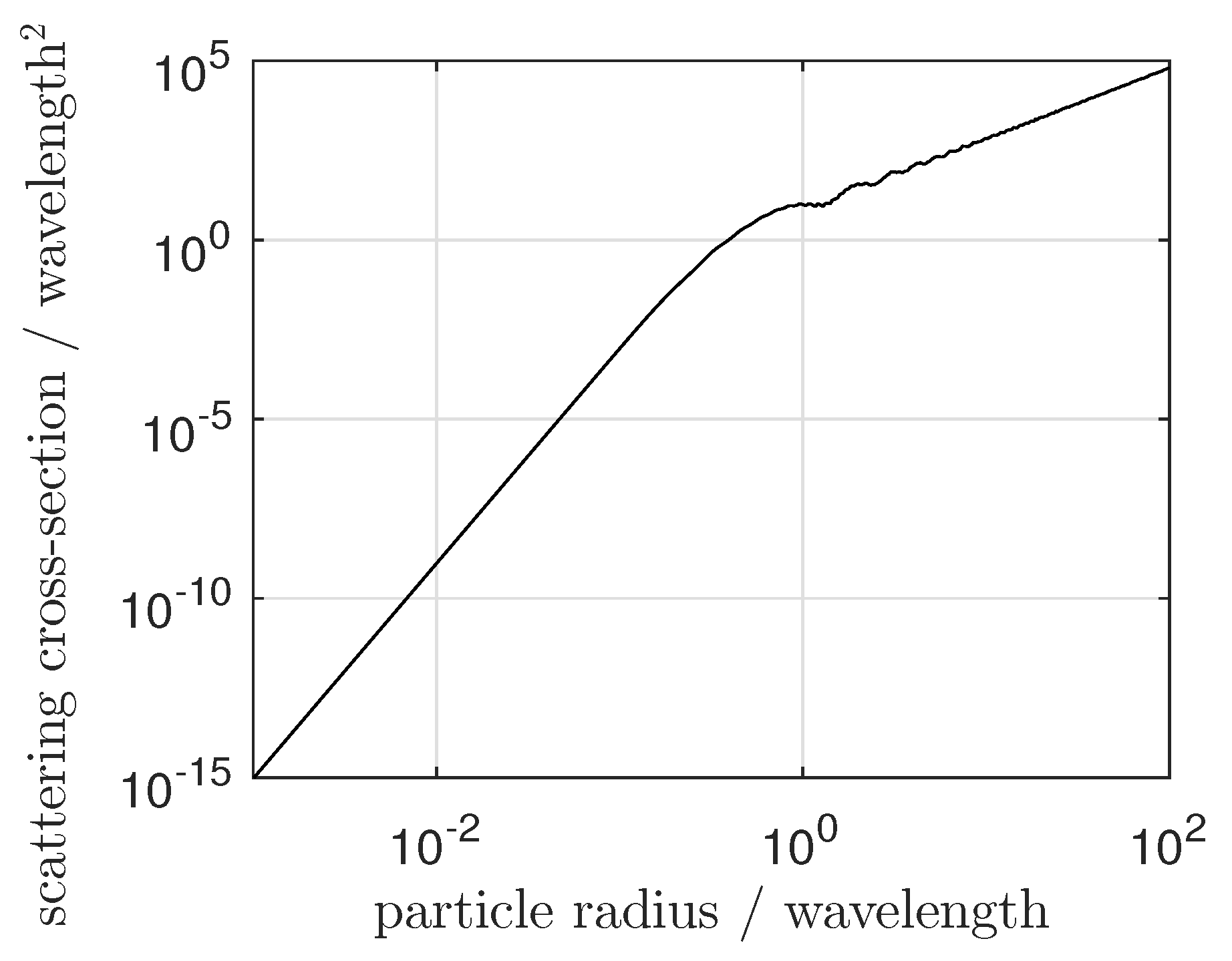
Figure 2.
Measurement arrangement of Doppler principles illustrated for the light scattering on a single particle (measurement of one velocity component, acceleration neglected).
Figure 2.
Measurement arrangement of Doppler principles illustrated for the light scattering on a single particle (measurement of one velocity component, acceleration neglected).

Figure 3.
Measurement arrangement of time-of-flight principles illustrated for the position measurement of a scattering particle (measurement of one velocity component, acceleration neglected).
Figure 3.
Measurement arrangement of time-of-flight principles illustrated for the position measurement of a scattering particle (measurement of one velocity component, acceleration neglected).
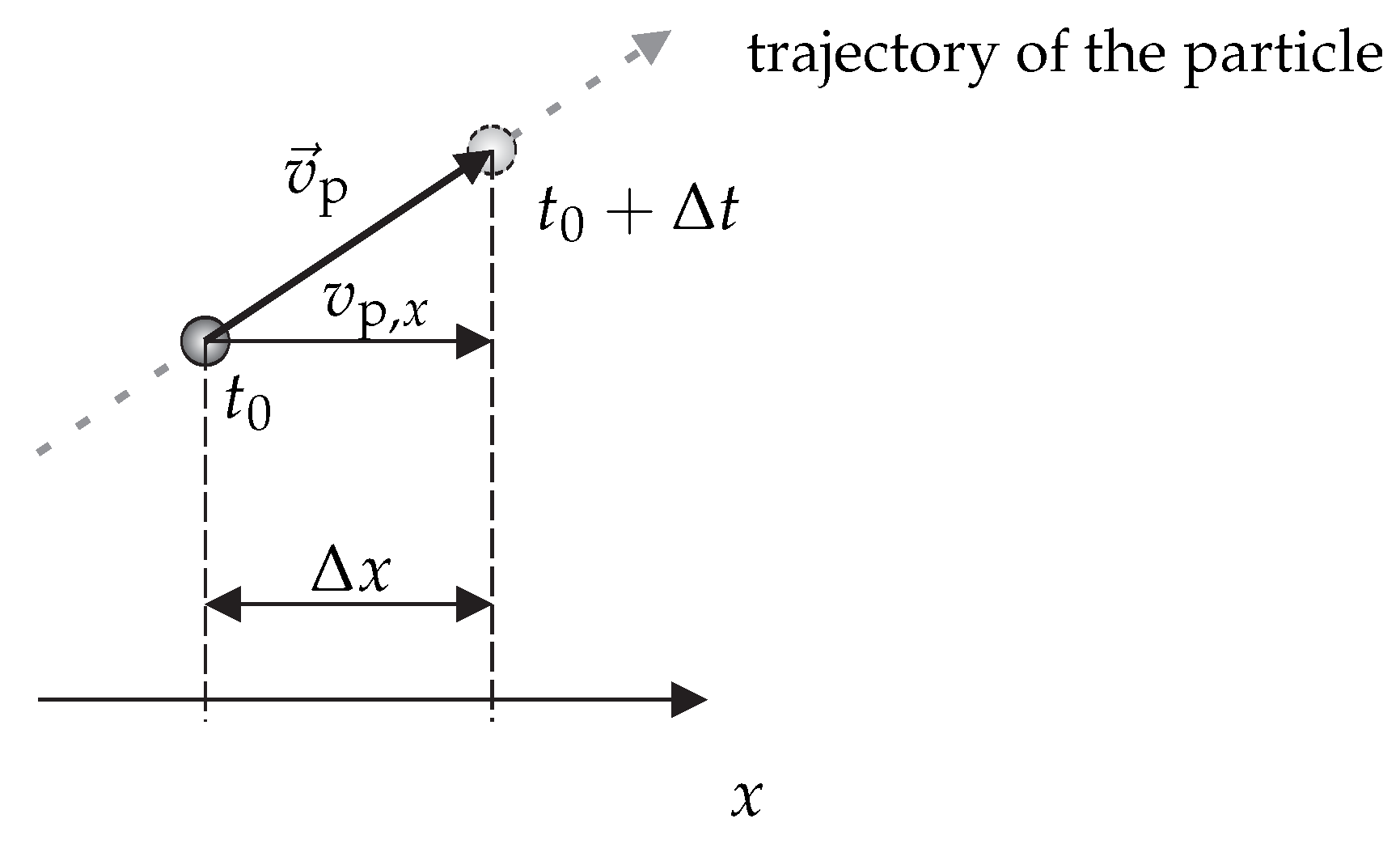
Figure 4.
Categorization of flow velocity measurement approaches based on Mie scattering.
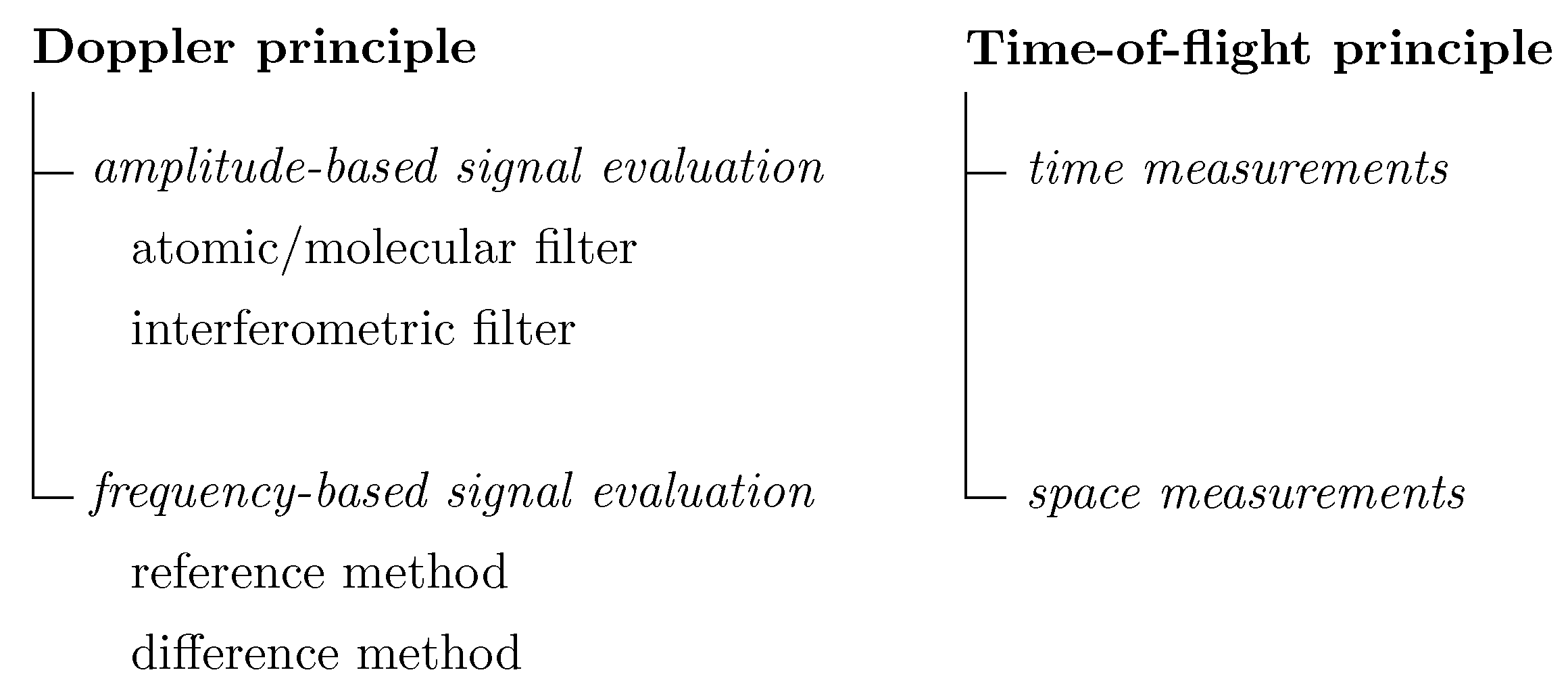
Figure 5.
Illustration of the terms (a) spatial resolution, spatial distance of the measurements and size of the measurement volume along one space dimension and (b) temporal resolution, measurement rate and measurement duration.
Figure 5.
Illustration of the terms (a) spatial resolution, spatial distance of the measurements and size of the measurement volume along one space dimension and (b) temporal resolution, measurement rate and measurement duration.

Figure 6.
(a) Change of the mean density of the fluid due to the seeding and (b) volume percentage of the seeding over the particle concentration.
Figure 6.
(a) Change of the mean density of the fluid due to the seeding and (b) volume percentage of the seeding over the particle concentration.

Figure 7.
Mean free distance of the seeding particles divided by the particle diameter over the seeding particle concentration for two different particle diameters.
Figure 7.
Mean free distance of the seeding particles divided by the particle diameter over the seeding particle concentration for two different particle diameters.
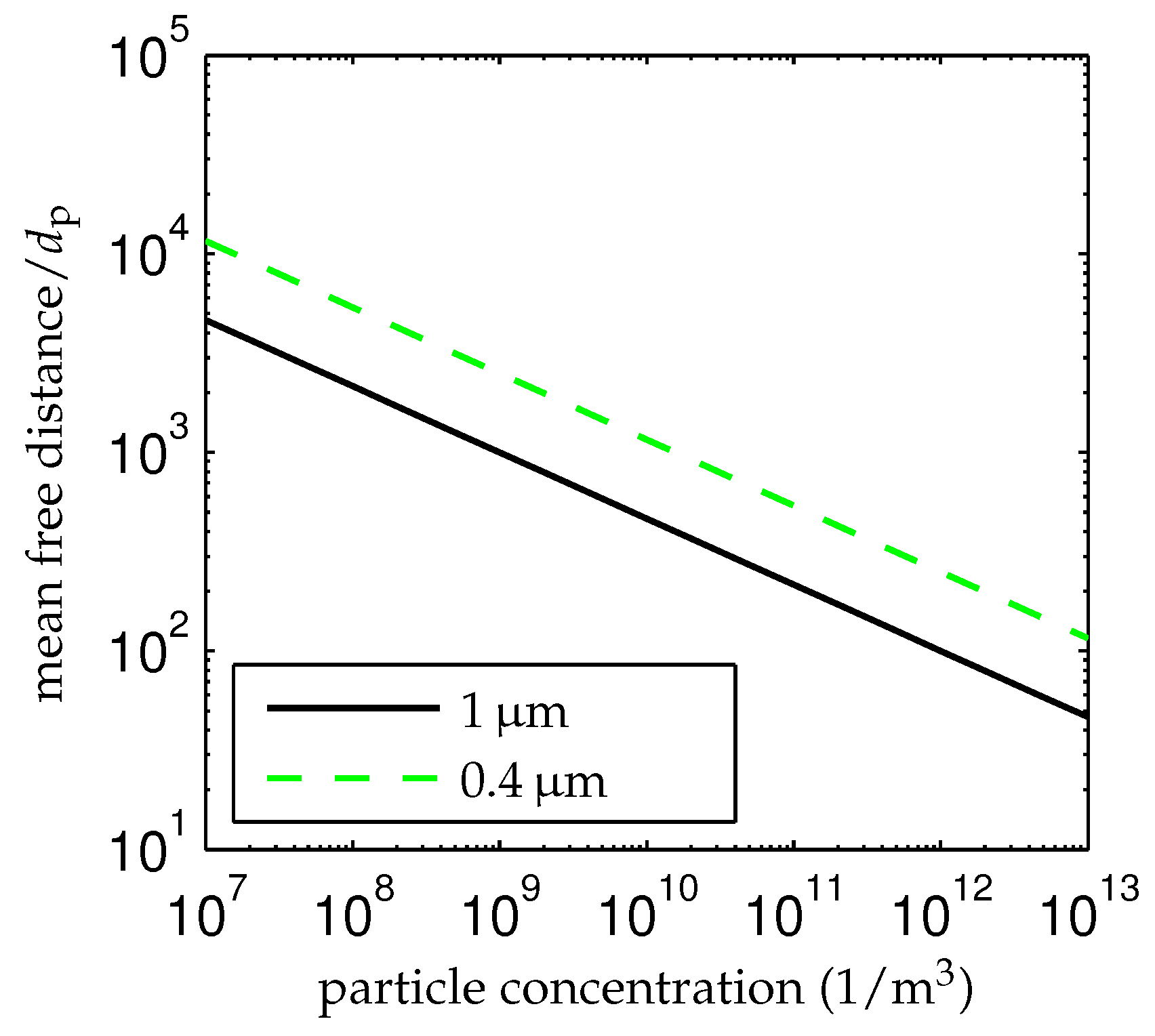
Figure 8.
Deviation of (a) the amplitude and (b) the phase of a cosinusoidal excitation due to the particle-following behavior of the particles listed in Table 1.
Figure 8.
Deviation of (a) the amplitude and (b) the phase of a cosinusoidal excitation due to the particle-following behavior of the particles listed in Table 1.

Figure 9.
Minimal achievable measurement uncertainty due to photon shot noise over the flow velocity v for an average photon rate per particle of (a) for a single particle (that passes the measurement volume with the respective dimension ) and (b) for multiple particles (that occur during the measurement time ). The formulas are from Table 2 and , , , , 2 GHz.
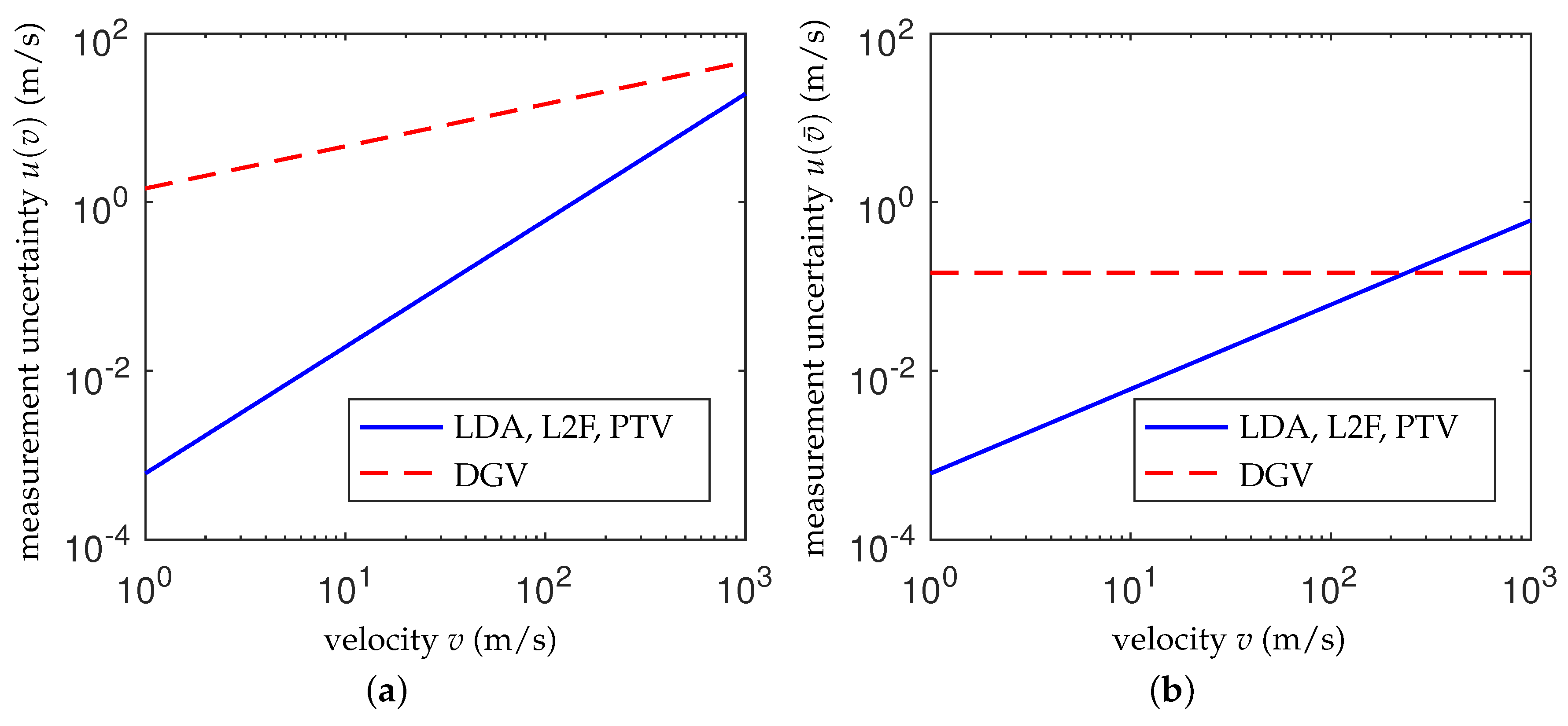

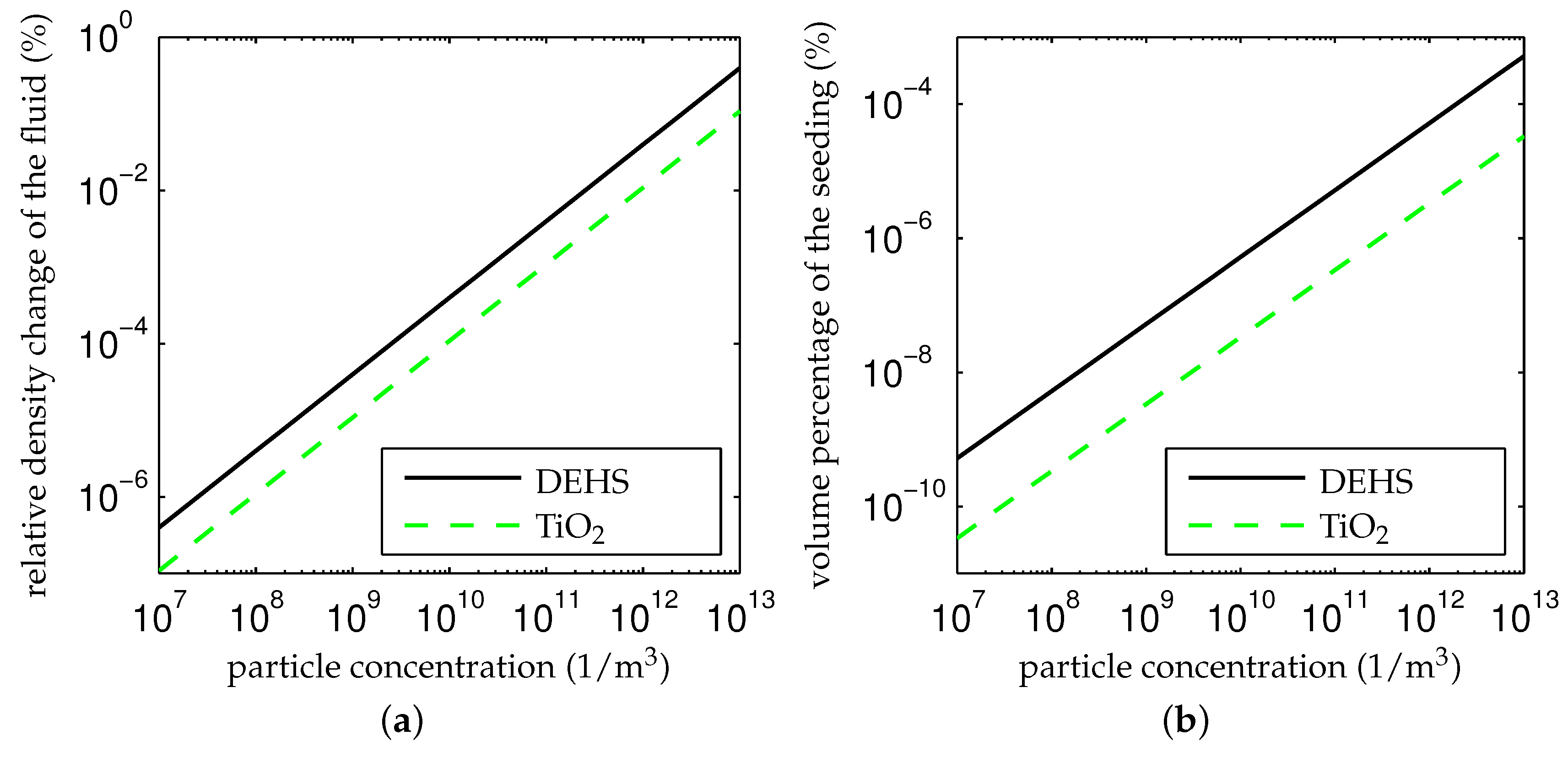
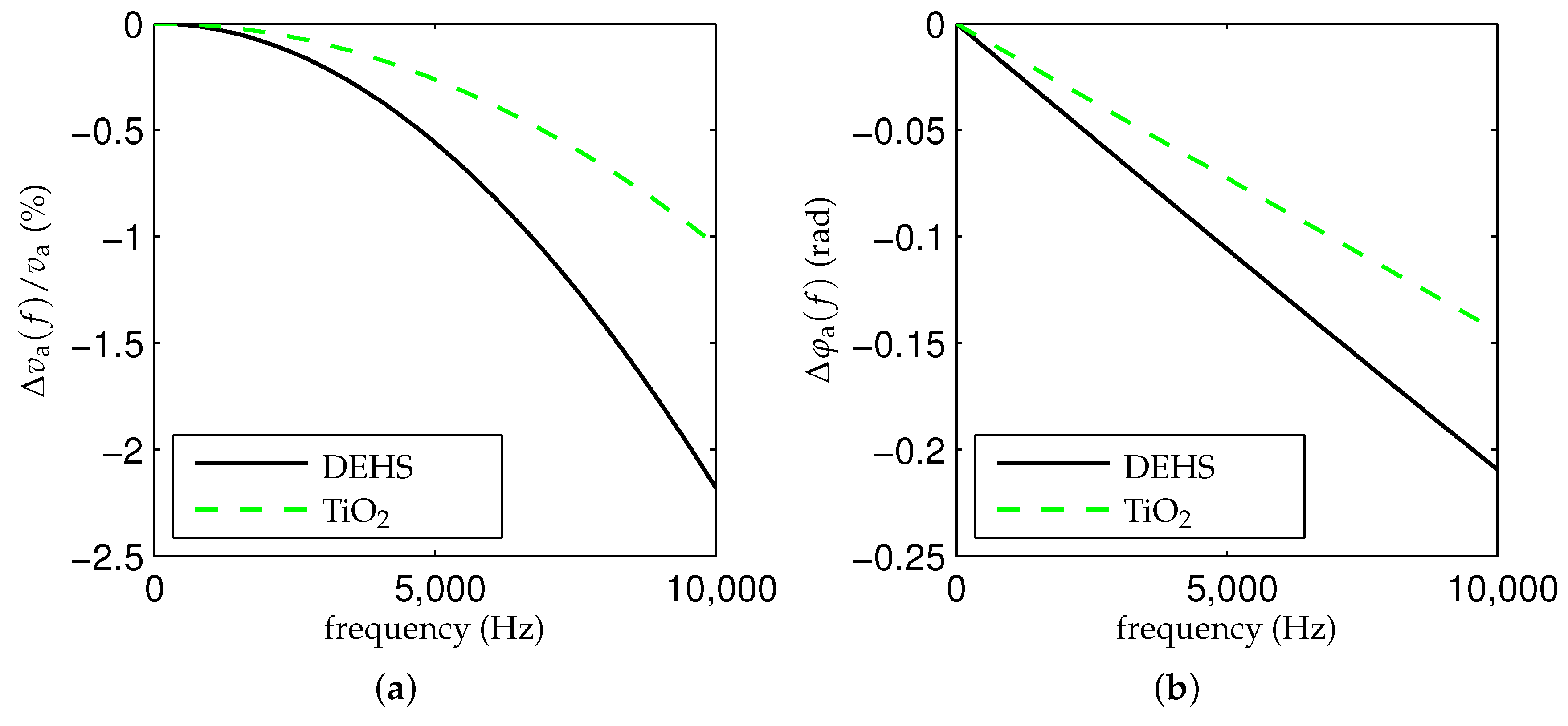
Table 1.
Material, density and diameter of two typical seeding particles.
| Material | (kg/m) | (m) |
|---|---|---|
| diethylhexyl sebacate (DEHS) | 912 | 1 |
| titanium dioxide (TiO) | 3900 | 0.4 |
Table 2.
Square root of the Cramér–Rao bound due to photon shot noise for Doppler and time-of-flight measurement techniques, which is the minimal achievable measurement uncertainty for a single particle and for multiple particles, respectively. DGV, Doppler global velocimetry; LDA, laser Doppler anemometer; L2F, laser-2-focus anemometry; PTV, particle tracking velocimetry.
| for a Single Particle | for Multiple Particles | ||
|---|---|---|---|
| DGV | |||
| LDA | |||
| L2F | |||
| PTV |
© 2017 by the author. Licensee MDPI, Basel, Switzerland. This article is an open access article distributed under the terms and conditions of the Creative Commons Attribution (CC BY) license (http://creativecommons.org/licenses/by/4.0/).
Share and Cite
MDPI and ACS Style
Fischer, A. Imaging Flow Velocimetry with Laser Mie Scattering. Appl. Sci. 2017, 7, 1298. https://doi.org/10.3390/app7121298
AMA Style
Fischer A. Imaging Flow Velocimetry with Laser Mie Scattering. Applied Sciences. 2017; 7(12):1298. https://doi.org/10.3390/app7121298
Chicago/Turabian StyleFischer, Andreas. 2017. "Imaging Flow Velocimetry with Laser Mie Scattering" Applied Sciences 7, no. 12: 1298. https://doi.org/10.3390/app7121298
Note that from the first issue of 2016, this journal uses article numbers instead of page numbers. See further details here.