Fault Diagnosis Model of Photovoltaic Array Based on Least Squares Support Vector Machine in Bayesian Framework

School of Electrical and Electronic Engineering, North China Electric Power University, Changping District, Beijing 102206, China
*
Author to whom correspondence should be addressed.
Appl. Sci. 2017, 7(11), 1199; https://doi.org/10.3390/app7111199
Submission received: 30 September 2017
/
Revised: 8 November 2017
/
Accepted: 20 November 2017
/
Published: 21 November 2017
Abstract
:With the rapid development of the photovoltaic industry, fault monitoring is becoming an important issue in maintaining the safe and stable operation of a solar power station. In order to diagnose the fault types of photovoltaic array, a fault diagnosis method that is based on the Least Squares Support Vector Machine (LSSVM) in the Bayesian framework is put forward. First, based on the elaborate analysis of the change rules of the output electrical parameters and the equivalent circuit internal parameters of photovoltaic array in different fault states, the input variables of the photovoltaic array fault diagnosis model are determined. Second, through the LSSVM algorithm in the Bayesian framework, the fault diagnosis model based on the output electrical parameters and the equivalent circuit internal parameters of the photovoltaic array is built, which can effectively detect the photovoltaic array faults of short circuit, open circuit, and abnormal aging. Then, the simulation model is built to verify the validity of the LSSVM algorithm in the Bayesian framework by comparing it with the model of LSSVM and the Support Vector Machine (SVM). Moreover, a 5 × 3 photovoltaic array and a reference photovoltaic string are established and experimentally tested to validate the performance of the proposed method.
1. Introduction
With the aggravation of the global energy crisis and regional environmental pollution, Chinese photovoltaic power generation still faces key problems of sustainable development [1], of which maintaining solar power station safety and maintaining stable operations are important issues. At present, research on solar power station fault monitoring is mainly focused on the photovoltaic strings, modules, and inverters, but rarely on the photovoltaic arrays. The diagnosis of the photovoltaic arrays is an important issue, because the performance of photovoltaic modules affects the output characteristics of photovoltaic arrays directly, thus further affecting the stability of the photovoltaic generation system, so the fault monitoring of the solar power station can diagnose the photovoltaic arrays, locate the faulty photovoltaic modules in a certain area first, and then further precisely position the faulty photovoltaic modules. This diagnostic method can greatly reduce the number of sensors, thus reducing costs while ensuring that the solar power station operates safely and stably.
In recent years, many fault detection and diagnosis methods of photovoltaic systems were proposed. The algorithm of the artificial neural network was presented to diagnose the fault [2,3,4,5]. In [6], the identification of the fault type is carried out by analyzing and comparing the amount of error deviations of both simulated and measured current and voltage with respect to a set of error thresholds that are evaluated. In [7], a simple method to detect and diagnose short circuits and open circuit faults in photovoltaic systems based on the evaluation of three coefficients is presented. By analyzing the light and dark current-voltage (I-V) characteristics of the photovoltaic module, a fault identification method was used to distinguish the faulty photovoltaic modules [8]. The above-mentioned methods are for the photovoltaic modules, of which each photovoltaic module needs to be monitored, leading to high costs. In [9,10,11,12,13], the fault diagnosis methods of the photovoltaic arrays were introduced. The fault detection is based on the comparison between the measured and model prediction results of the power production [9]. Hu, YH, et al., analyze the terminal characteristics of faulty photovoltaic arrays and reduce the number of sensors by optimizing its locations [10]. In [11], the authors diagnose the fault by detecting the change of PV internal resistance using the signals that are available in Extremum-Seeking Control (ESC)-based Maximum Power Point Tracking (MPPT). The methods in these works can only identify whether there is a fault or not, but the fault type is unknown. In other research [12], a method is proposed to detect faults and partial shading under all of the irradiation conditions using the measured values of array voltage, array current, and irradiance, but the diagnosis of fault type is not comprehensive enough.
In order to diagnose whether there are faulty photovoltaic modules in a photovoltaic array or not and further judge its fault type, this paper presents a fault diagnosis method that is based on Least Squares Support Vector Machine (LSSVM) in the Bayesian framework. The algorithm of LSSVM in the Bayesian framework has been used in the field of fault diagnosis, in domains such as aeronautics, power transformation, biology, and so on [13,14,15,16]; in this work, we introduce the algorithm into the field of photovoltaic fault diagnosis.
2. The Selection of the Fault Feature
This paper mainly focuses on the fault types of photovoltaic array: short circuit, open circuit, and photovoltaic modules’ abnormal aging. By analyzing the different fault types of photovoltaic array, we can obtain the change laws of the output characteristics and equivalent circuit internal parameters of photovoltaic array in different fault conditions, providing a theoretical basis and fault feature information for the diagnosis and location of photovoltaic array.
2.1. Analysis of Internal Parameters of Photovoltaic Array Equivalent Circuit in Fault State
If the photovoltaic array malfunctions, the internal parameters of the photovoltaic array equivalent circuit will change, and these differences contain the most abundant fault feature information, directly reflecting the state that the photovoltaic array is in.
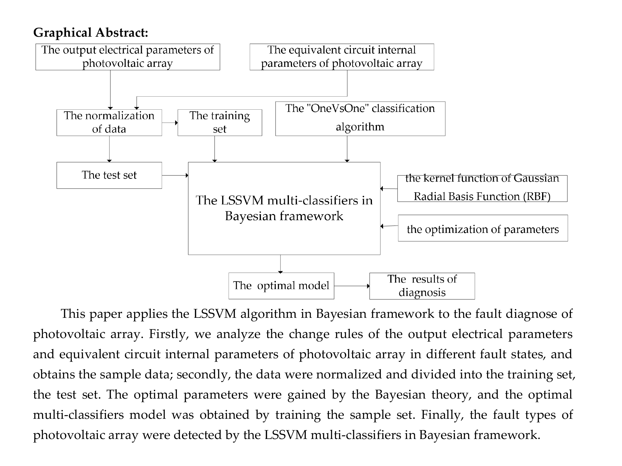
Figure 1 presents the equivalent circuit model of photovoltaic module [17], Iρh is the photovoltaic current generated by the photovoltaic module, ID is the current through the diode, Ish is the current flowing through the shunt resistance Rsh, Rs is the series resistance, and I is the output current of the photovoltaic module.
As the equivalent circuit model of photovoltaic module shows that the photovoltaic module output current is:
In the Formula, I0 is the reverse saturation current of the diode, U is the output voltage of the photovoltaic module, q is the electron charge ( Coulomb), n is the ideality factor of the diode, k is the Boltzmann’s constant ( J/K), and T is the absolute temperature of photovoltaic module.
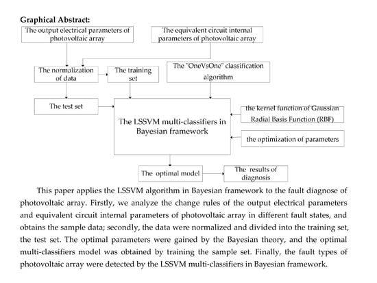
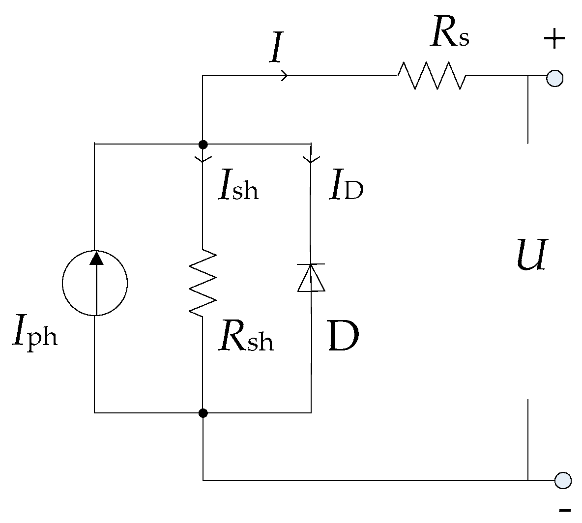
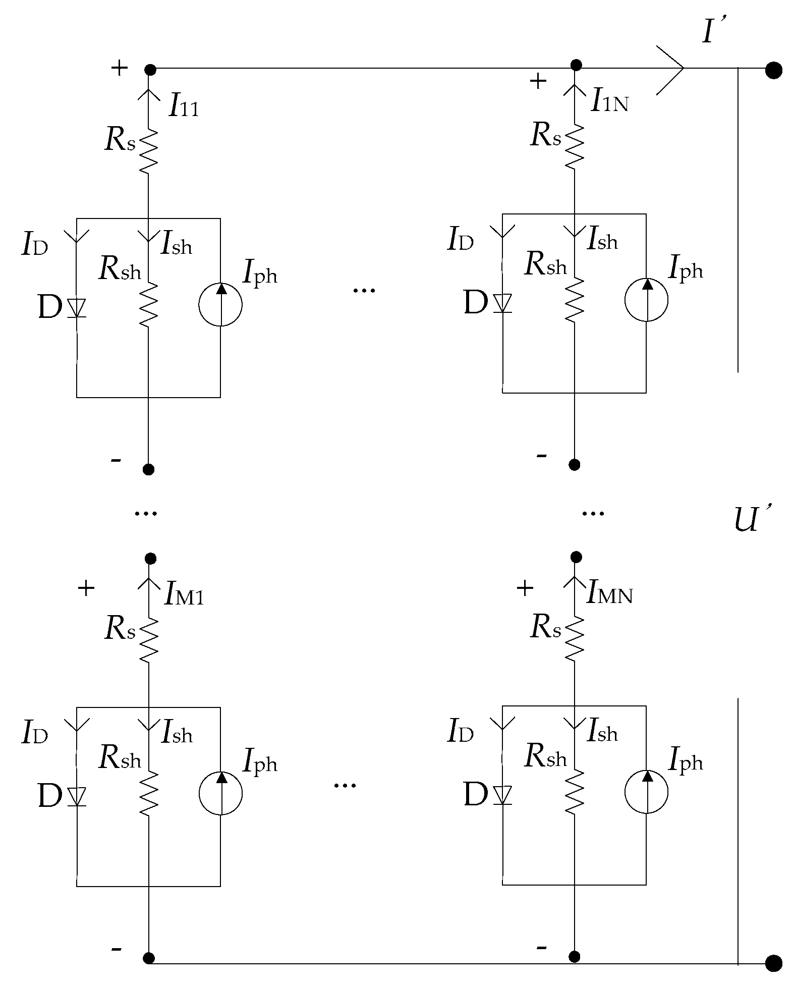
In an actual solar power station, there are five major connection types of photovoltaic array: series structure, parallel structure, serial-parallel (SP) structure, total-cross-tied (TCT) structure, and bridge-linked (BL) structure, among which the SP structure is the most widely used; therefore, this paper studies the photovoltaic array of the SP structure. Figure 2 is an equivalent circuit model of photovoltaic array, of which the type of the photovoltaic array is M × N, M is the number of photovoltaic modules in a photovoltaic string, and N is the number of photovoltaic strings in a photovoltaic array.
I’, U’ are the output current and voltage of the photovoltaic array, respectively; Iρh’ is the photovoltaic current generated by the photovoltaic array; and, Rs’, Rsh’ are the series resistance and shunt resistance of the photovoltaic array, respectively.
In the literature [18], the output current of photovoltaic array is:
The above analysis shows that , , and . For the model, its internal equivalent parameters Iρh’, Rs’, and Rsh’ is proportion to Iρh, Rs, and Rsh of the photovoltaic module.
From Figure 1, Figure 2 and Figure 3 and the above analysis, it shows that under the same test condition, Iρh, Rs, and Rsh of the faulty photovoltaic module are zero when there is a short-circuit fault in the photovoltaic array; thus, the Iρh of its string keeps constant, Rs and Rsh decreases, and then the Iρh’ is basically unchanged, while Rs’ and Rsh’ decrease.
When there is an open-circuits photovoltaic module in the photovoltaic array, the Iρh, Rs, and Rsh of its string are zero, and the internal parameters of photovoltaic array equivalent circuit are:
Of which, is the number of photovoltaic strings that has open-circuits. In this case, the Iρh’ decreases, while Rs’ and Rsh’ increase.
From the above analysis and the literature [19], we know that when a photovoltaic module in photovoltaic array is abnormally aging, so its Iρh, Rsh decreases, Rs increases, the Iρh’, Rsh’ of photovoltaic array equivalent circuit decreases, and Rs’ increases.
Therefore, the Iρh’, Rs’, and Rsh’ of photovoltaic array equivalent circuit can be used as the parameters of the photovoltaic array fault diagnosis model, which can effectively identify the faults of short circuit, open circuit, and abnormal aging.
2.2. Analysis of the Output Characteristics of Photovoltaic Array in Fault State
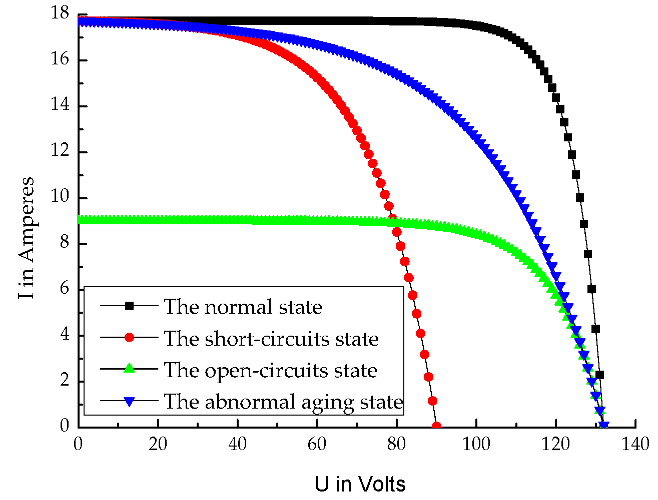
When the photovoltaic array fails, different fault types have different influences on the output of photovoltaic array. Figure 4 shows the I-V curves of the 3 × 2 photovoltaic array in normal and different fault conditions, of which the photovoltaic modules are in same test conditions (1000 W/m2, 25 °C); the model of photovoltaic module is CHN310-72P.
Figure 4 shows that when the fault of short-circuits occurs in the photovoltaic array, the short-circuit current ISC and maximum power current Im are basically unchanged, while the open-circuit voltage UOC and the maximum power voltage Um are significantly decreased. When the fault of short-circuits occurs in the photovoltaic array, the current of faulty photovoltaic module is zero; then, the current and voltage of its string decreases, resulting in a decrease in the output voltage of the photovoltaic array. From the I-V characteristic curve of a photovoltaic cell, we can know that when the output voltage of normal string reduces, its output current will increase, resulting in little change in the total output current of photovoltaic array.
When the fault of open-circuits occurs in the photovoltaic array, the open-circuit voltage UOC and maximum power voltage Um are basically unchanged, while the short-circuit current ISC and the maximum power current Im significantly decrease. When the fault of open-circuits occurs in the photovoltaic array, the current of its string is zero, which causes the output current of the photovoltaic array to decrease dramatically, and the output voltage of normal strings and the photovoltaic array are basically unchanged.
When the photovoltaic modules in the photovoltaic array are abnormally aged, the open-circuit voltage UOC and short-circuit current ISC are basically unchanged, while the maximum power voltage Um and the maximum power current Im significantly decrease. The literature [20] points out that the open-circuit voltage UOC and the short-circuit current ISC contain the information of temperature and light intensity. The above analysis and the literature [20] show that the open-circuit voltage UOC, the short-circuit current ISC, the maximum power voltage Um, and the maximum power current Im can be regarded as the external characteristic parameters of the photovoltaic array fault diagnosis model.
3. The Establishment of the Photovoltaic Array Fault Diagnosis Model
The key of establishing the photovoltaic array fault diagnosis model is the optimal LSSVM multi-classifiers; the output electrical parameters and equivalent circuit internal parameters of photovoltaic array we attained are input into the optimal multiple classifiers model, thus obtaining the posteriori probabilities of the photovoltaic array and further detecting the fault types of the short circuit, open circuit, and abnormal aging.
In the process of the optimal LSSVM multi-classifiers model being built, we established an initial model first, and then the Bayesian theory was used to optimize the parameters of the initial model. Empirical results obtained from 10 public domain data sets show that the LSSVM classifier designed within the Bayesian evidence framework consistently yields good generalization performances and prediction precision [21].
3.1. The Establishment of the Initial LSSVM Multi-Classifiers Model
3.1.1. The Method of LSSVM Classifier
In [22], J.A.K. Suykens and J. Vandewalle present the LSSVM, which uses the least squares linear system error square and loss function as the empirical loss of training sample set, changing the constraint condition from inequation to equation; then, the convex quadratic programming problem transforms and is able to solve the problem of linear equations, and calculation speed of the model is improved.
The objective function and constraint condition of LSSVM are:
In the above linear equations, is the weight vector, C is the penalty factor, g is the number of training samples, ε is slack variable, εi is the ith component of the slack variable ε, xi Rm is the training sample, and m is the dimension of the training sample’s feature vectors; in this paper, xi presents the output characteristics UOC, ISC, Um, Im and equivalent circuit internal parameters Iρh’, Rs’, Rsh’ of photovoltaic array; yi y = {1,−1} is the output; yi presents the states of short circuit, open circuit, abnormal aging, and normal; b is the classification threshold.
The above optimization problem is the convex quadratic programs of and b, so we introduce the Lagrangian function, which can be constructed as follows:
In the Formula (7), α is the Lagrangian multiplier, and K (xi, xj) is the kernel function.
The Lagrangian function converts the primal problem (6) into the dual problem (8)
Through Equation (8), we can get:
The optimal hyperplane is constructed, then the decision function is obtained:
Through the above problem-solving procedure, the LSSVM multi-classifiers model is built. In order to obtain the optimal LSSVM multi-classifiers, we can optimize the parameters of C and K (xi, xj).
3.1.2. The Initial LSSVM Multi-Classifiers Model
The basic idea of the kernel function K (xi, xj) is for mapping the random vectors in n-dimensional space to the high-dimensional feature space by nonlinear function, which can reduce the dimensionality.
In practice, there are three most common kernel functions: the polynomial kernel function, the Radial Basis Function (RBF), and the Sigmoid kernel function. Keerthi et al., testified that the polynomial kernel function is the special form of the RBF kernel function [23]. In [24], the Sigmoid kernel function is similar to the RBF kernel function in some cases, so, in this work, the RBF kernel function is used as the kernel function of the photovoltaic array fault diagnosis model.
where σ is the kernel parameter of K (xi, yi).
For the sake of processing, the objective function of the LSSVM optimization problem is divided by C, and 1/C is replaced by θ, which is defined as regularization parameter.
First, we set the initial values of θ and σ2 arbitrarily, and establish the initial model H0 to train the training set.
The SVM and LSSVM were presented for secondary classification initially, but the photovoltaic array fault diagnosis model is a multi-classification problem; thus, the classification algorithm can be used to convert the multi-classifiers into several two-classifiers. The common classification algorithms are “One vs. One”, “One vs. Rest”, and “Divide-and-Conquer approach”; the algorithm of “One vs. One” is better than the “One vs. Rest” in diagnosis efficiency, and the algorithm of “Divide-and-Conquer approach” can lead to accumulations of errors—that is, if the classification of root is wrong, then the error will accumulate [25], so we use the “One vs. One” classification algorithm in the LSSVM multi-classifiers.
In this paper, the LSSVM multi-classifiers were converted into six two-classifiers by the classification algorithm of “One vs. One”, which are “the normal vs. the short-circuits”, “the normal vs. the open-circuits”, “the normal vs. the abnormal aging”, “the short-circuits vs. the open-circuits”, “the short-circuits vs. the abnormal aging”, and “the open-circuits vs. the abnormal aging”.
3.2. The Posteriori Probability of the Optimal LSSVM Multi-Classifiers
Based on the posteriori distribution, which synthesized the sample information and the a priori information, the Bayesian inference has good statistical inference results. In this paper, Bayesian theory is used to optimize the parameters of the LSSVM classifier, regularization parameter θ, and kernel parameter σ; it then obtains the optimal classifier.
The LSSVM achieves pattern recognition by hard decision, that is, it classifies the sample by outputting 1 or −1 directly; however, pattern recognition is an uncertain problem, so this paper diagnoses the fault by the output probability of LSSVM.
For a given sample set T = {(x1, y1), …, (xg, yg)} (Rm × y)g, in this paper, xi presents the parameters UOC, ISC, Um, Im, Iρh’, Rs’, Rsh’ of photovoltaic array, yi presents its real states of short circuit, open circuit, abnormal aging, and normal.
The posterior probability of the given sample set can be described as:
In the Formula (11), P(y) is the a priori probability of the given sample set, which analyzes the probability of a sample according to the a priori knowledge; P(y|x) is the posteriori probability of the given sample set according to the training set, and the posteriori probability reflects the influence of the training sample data on the test sample.
In this paper, the posteriori probability of the given sample set is:
In the Formula (12), D1 is the given sample data space, and H is the fault diagnosis model space.
A posteriori probability is derived from the two-classifiers. According to the above analysis, we can know that the photovoltaic array fault diagnosis model constructs six two-classifiers, so six posteriori probabilities can be generated from the sample data. Then, by combining the posteriori probabilities by the Formula (13), we can get four combination probabilities.
The final posteriori probability of determining the test sample x belonging to the i-class is:
In Formula (13), Pij(i, j|x) is the posteriori probability of x that belongs to the i-class in two-classifiers that consist of class i and j class, and L is the sort of photovoltaic array it is in. In this paper, L is 4; they are the states of short circuit, open circuit, abnormal aging, and normal.
When comparing the size of the four combination probabilities, we can judge the fault type of the testing set.
4. Simulation and Results
In this section, several data sets are constructed to study the performance of the fault diagnosis method. We first introduce the construction of a simulation system, then the test data under different states are simulated and briefly described. Finally, the simulation results are presented.
4.1. The Simulation of Photovoltaic System
In order to verify the validity of LSSVM algorithm based on Bayesian framework in photovoltaic array fault diagnosis model, this paper sets up a general simulation model of photovoltaic array by Matlab/Simulink; the photovoltaic array consists of two photovoltaic strings in parallel, and each string has three modules in series.
4.2. The Simulation Data in Different States
In the photovoltaic array simulation model, the fault of abnormal aging is simulated by connecting a series resistor. The model of photovoltaic modules in the simulation model is CHN310-72P, and the main parameters of the photovoltaic module at standard test conditions (STC) are shown in Table 1.
The outputs of the simulation model are the operating voltage U and the output current I of the photovoltaic array; thus, we can obtain the V-I curve of the photovoltaic array under the STC, which further gets the external parameters Uoc, Isc, Um, Im, and the equivalent circuit internal parameters Iρh’, Rs’, Rsh’ [26]. From the simulation results, we can know that the external parameters of photovoltaic array in normal state are: Uoc = 121.00 V, Isc = 15.85 A, Um = 107.00 V, and Im = 15.90 A, and the equivalent circuit internal parameters are: Iρh’ = 16.68 A, Rs’ = 0.21 Ω, and Rsh’ = 8.12 KΩ. The comparison studies show that the parameters obtained by the simulation are basically consistent with the parameters that are provided by the manufacturer, which shows that the model can simulate the actual photovoltaic array well.
The photovoltaic array runs in the states of normal, short circuit, open circuit, and abnormal aging; 40 sample groups in each state (160 sample groups altogether) were obtained, of which 30 sample groups were used as the training set, and the remaining 10 groups were used as the testing set.
4.3. The Standardization Analysis of the Data
Firstly, we imported the fault features to the data editor and normalized the sample data. Saving the standardization scores as a variable, the results of sample data standardization analysis are shown in Table 2; it shows the standardization data of the fault features of 10 test sample groups in short-circuits state.
4.4. Results Analysis
This paper classifies the sample data by the Lssvmlab v 1–8 toolbox in Matlab R2014a environment, of which the Gaussian RBF is used as the kernel function and the “One vs. One” classification algorithm is used to build the LSSVM multi-classifiers model.
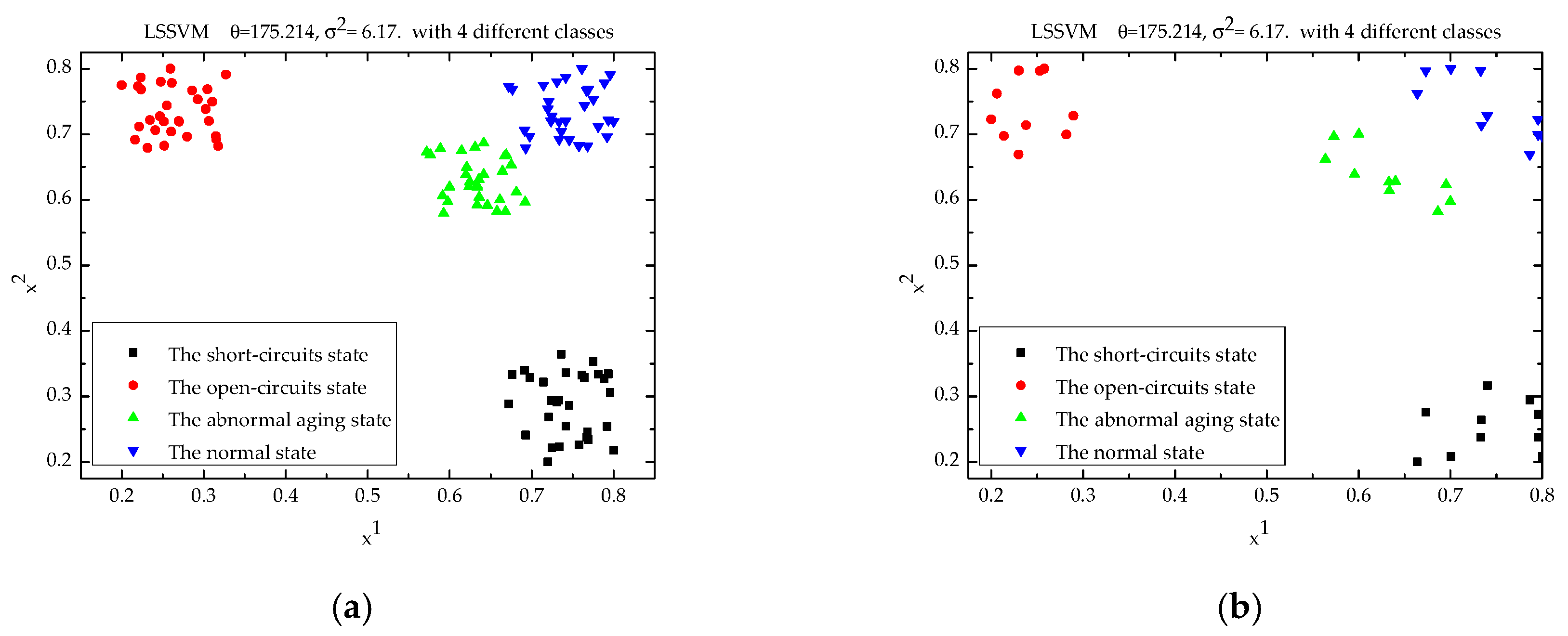
This paper establishes the initial model H0 first; the regularization parameter θ is set to 10 and the kernel parameter σ2 is 0.2. Furthermore, the Bayesian inference is used to optimize the parameters of the model and to obtain the optimal parameters (θMP, σ2MP) = (175.214, 6.17); then, the optimal model is obtained by re-training the training set with the optimal parameters θMP and σ2MP. Finally, the testing set is input into the optimal classifier model and obtains the posteriori probability and classification.
In this paper, the LSSVM multi-classifiers were converted into six two-classifiers by the classification algorithm of “One vs. One”, which consists of “1&2”, “1&3”, “1&4”,”2&3”, “2&4”, and ”3&4”. The output posteriori probability values of 10 test sample groups in short-circuits state are shown in Table 3, of which 1 represents the short-circuits state, 2 represents the open-circuits state, 3 represents the abnormal aging state, and 4 represents the normal state.
The posteriori probabilities in Table 3 were combined by the Formula (13) and get the final posteriori probabilities of the 10 test sample groups. The actual fault type was obtained by the size of the final posteriori probability, as shown in Table 4. The Table illustrates the actual fault type and the fault type of diagnosis of the 10 test sample groups.
Figure 5 is the multi-classification diagram based on Bayesian theory, Figure 5a is the multi-classification diagram of the training set, and Figure 5b is the multi-classification diagram of the testing set. x1, x2 are the feature vectors whose dimension is reduced by the RBF kernel function.
Compared the LSSVM algorithm in Bayesian theory with the LSSVM algorithm and the standard SVM algorithm, the results are as shown, in Table 5.
Among the LSSVM algorithm and the standard SVM algorithm, the RBF is the kernel function, the classification algorithm is the “One vs. One”, the difference is that the optimization method of the regularization parameter , and the kernel parameter is the 10 times cross-validation method. O is the total number of test samples, and Percent is the proportion of the well-judged test samples and the total test samples. The results show that the LSSVM in Bayesian theory has higher generalization ability and good modeling effect.
5. Experimental Results
In this section, the presented fault diagnosis model is tested with an experimental photovoltaic system, and the experimental platform, as well as the experimental results, are presented.
5.1. Experimental Platform
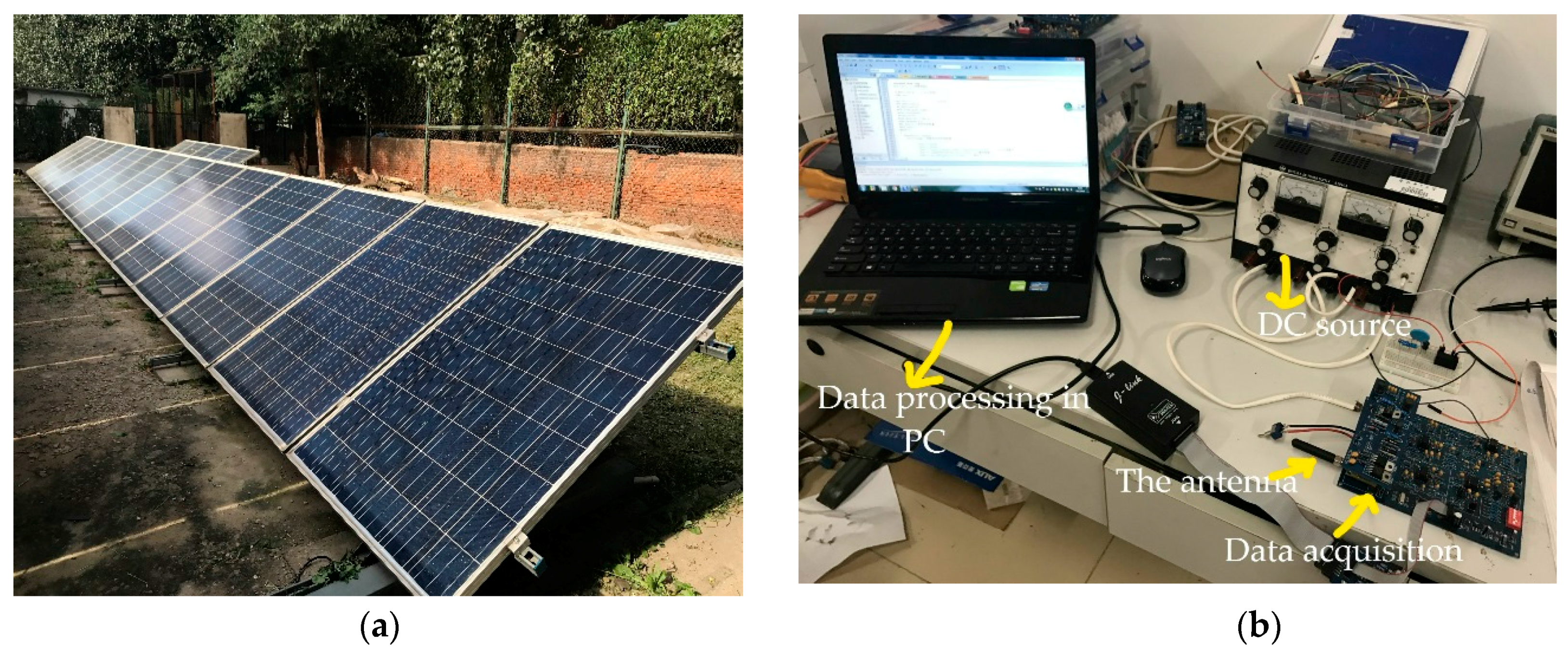
A 35 kW Experimental Substation is applied to validate the performances of the proposed fault diagnosis model. As Figure 6 shows, we take a photovoltaic string as experimental subject, which consists of sixteen modules in series. We took fifteen of them into a 5 × 3 photovoltaic array, which consists of three photovoltaic strings in parallel, and each string has five modules in series. A reference photovoltaic string behind experimental array is used for comparison, which consists of five modules. The solar irradiance (G) is collected by the illumination intensity detector TBQ-2 (Beijing Huatron Technology Co., Ltd., Beijing, China), and the ambient temperature (T) is collected by the temperature sensor PT100 (Haodu Sensors Technology Co., Ltd., Shenzhen, China). The current is provided by the DC (Direct Current) resource DH1718-A (Dahua Technology Co., Ltd., Beijing, China).
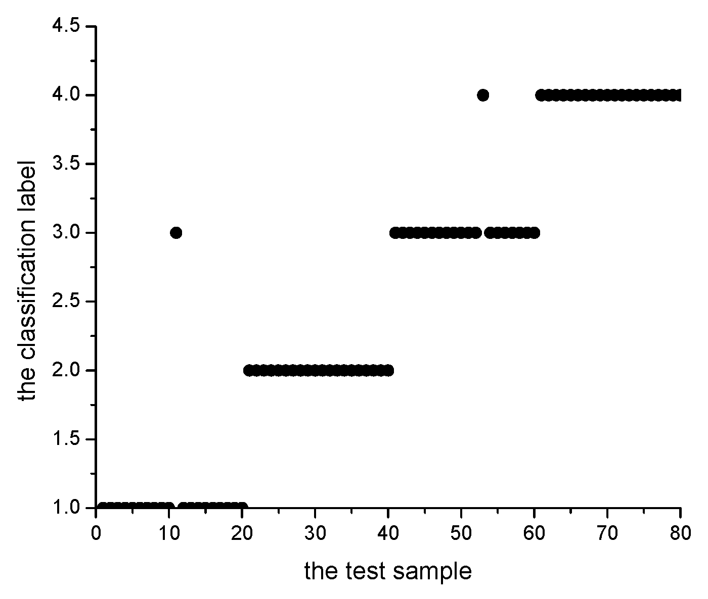
In the fault diagnosis model, the fault of abnormal aging is simulated by connecting a series resistor, while the fault of short circuit is simulated by paralleling a photovoltaic module with a constructor, disconnecting the constructor between two photovoltaic modules that represent the fault of open circuit. Four instances are implemented and studied, including in the states of normal, short circuit, open circuit, and abnormal aging. 80 sample groups in each state (320 sample groups altogether) were obtained, of which 60 sample groups were used as the training set, and the remaining 20 groups were used as the testing set.
5.2. Experimental Results
Table 6 demonstrates the final posteriori probabilities of six test samples in short-circuits state, while Figure 7 illustrates the experimental results of the aforementioned four instances, which demonstrate that the accuracy of the proposed method is 97.5%.
It is obvious that the experimental data can be classified by the fault diagnosis model in Bayesian theory, which is similar to the simulated ones.
6. Conclusions
According to the change rules of the output electrical parameters and the equivalent circuit internal parameters of the photovoltaic array in different fault states, a LSSVM multi-classifiers model in Bayesian theory has been built to diagnose the fault types of the photovoltaic array.
The proposed method has the ability to construct an optimal multiple-classifiers model and to obtain the posteriori probabilities of the samples, which can identify the states of the photovoltaic array. Four kinds of working conditions are simulated to validate the effectiveness of the approach—that is, the normal condition, the short-circuits condition, the open-circuits condition, and the abnormal aging condition. The simulated results indicate that the method can classify the fault types accurately, which have a higher generalization ability and a good modeling effect. Furthermore, an experimental platform is built to test the experimental performance of the developed approach, while the experimental results also demonstrate the effectiveness of the fault diagnosis model in a practical system.
This paper deeply analyzes the change rules of the output electrical parameters and the equivalent circuit internal parameters of the photovoltaic array in different fault states. It also introduces the Bayesian Framework for LSSVM into the field of photovoltaic fault diagnosis so that we can locate the faulty photovoltaic modules into a certain photovoltaic array and further diagnose its fault types, thus greatly reducing the number of sensors and the costs, while ensuring that the solar power station operates safely and stably.
Acknowledgments
This study was conducted as part of the project cooperated with the State Grid Corporation of Qinghai, China. It is also supported by the Fundamental Research Funds for the Central Universities (2016MS06).
Author Contributions
All authors contributed equally to this work. Fengjie Sun proposed the original idea. Jiamin Sun designed the overall framework of this paper, built the simulation model and completed the manuscript. Jieqing Fan modified and refined the manuscript. Yutu Liang conducted data analysis. All authors read and approved the final manuscript.
Conflicts of Interest
The authors declare no conflict of interest.
References
- Sahu, B.K. A study on global solar PV energy developments and policies with special focus on the top ten solar PV power producing countries. Renew. Energy 2015, 43, 621–634. [Google Scholar] [CrossRef]
- Rezgui, W.; Mouss, L.H.; Mouss, M.D.; Kadri, O.; DISSA, A. Electrical faults detection for the intelligent diagnosis of a photovoltaic generator. J. Electr. Eng. 2014, 14, 77–84. [Google Scholar]
- Chine, W.; Mellit, A.; Lughi, V.; Malek, A.; Sulligoi, G.; Pavan, A.M. A novel ault diagnosis technique for photovoltaic systems based on artificial neural networks. Renew. Energy 2016, 90, 501–512. [Google Scholar] [CrossRef]
- Jiang, L.L.; Maskell, D.L. Automatic fault detection and diagnosis for photovoltaic systems using combined artificial neural network and analytical based methods. In Proceedings of the 2015 International Joint Conference on Neural Networks (IJCNN), Killarney, Ireland, 12–17 July 2015; pp. 1–8. [Google Scholar]
- Mekki, H.; Mellit, A.; Salhi, H. Artificial neural network-based modelling and fault detection of partial shaded photovoltaic modules. Simul. Model. Prac. Theory 2016, 67, 1–13. [Google Scholar] [CrossRef]
- Silvestre, S.; Chouder, A.; Karatepe, E. Automatic fault detection in grid connected PV systems. Sol. Energy 2013, 94, 119–127. [Google Scholar] [CrossRef]
- Garoudja, E.; Kara, K.; Chouder, A.; Silvestre, S.; Kichou, S. Efficient fault detection and diagnosis procedure for photovoltaic systems. In Proceedings of the 2016 8th International Conference on Modelling, Identification and Control (ICMIC), Algiers, Algeria, 15–17 November 2016; pp. 851–856. [Google Scholar]
- Spataru, S.V.; Sera, D.; Hacke, P.; Kerekes, T.; Teodorescu, R. Fault identification in crystalline silicon PV modules by complementary analysis of the light and dark current-voltage characteristics. Prog. Photovolt. 2016, 24, 517–532. [Google Scholar] [CrossRef]
- Platon, R.; Martel, J.; Woodruff, N.; Chau, T.Y. Online fault detection in PV systems. IEEE Trans. Sustain. Energy 2015, 6, 1200–1207. [Google Scholar] [CrossRef]
- Hu, Y.H.; Zhang, J.F.; Cao, W.P.; Wu, J.D.; Tian, G.Y.; Finney, S.J.; Kirtley, J.L. Online two-section PV array fault diagnosis with optimized voltage sensor locations. IEEE Trans. Ind. Electron. 2015, 62, 7237–7246. [Google Scholar] [CrossRef]
- Li, X.; Li, Y.Y.; Seem, J.E.; Lei, P. Detection of internal resistance change for photovoltaic arrays using Extremum-Seeking control MPPT signals. IEEE Trans. Control Syst. Technol. 2016, 24, 325–333. [Google Scholar] [CrossRef]
- Hariharan, R.; Chakkarapani, M.; Ilango, G.S.; Nagamani, C. A method to detect photovoltaic array faults and partial shading in PV systems. IEEE J. Photovolt. 2016, 6, 1278–1285. [Google Scholar] [CrossRef]
- Khawaja, T.; Vachtsevanos, G. A novel bayesian least squares support vector machine based anomaly detector for fault diagnosis. In Proceedings of the Annual Conference of the Prognostics and Health Management Society (PHM 2009), San Diego, CA, USA, 27 September–1 October 2009. [Google Scholar]
- Luts, J.; Ojeda, F.; Van de Plas, R.; De Moor, B.; Van Huffel, S.; Suykens, J.A.K. A tutorial on support vector machine-based methods for classification problems in chemometrics. Anal. Chim. Acta 2010, 665, 129–145. [Google Scholar] [CrossRef] [PubMed]
- Khawaja, T.S. A Bayesian Least Squares Support Vector Machines Based Framework for Fault Diagnosis and Failure Prognosis. Ph.D. Thesis, Georgia Institute of Technology, Atlanta, GA, USA, August 2010. [Google Scholar]
- Liu, C.; Kong, D.W.; Fan, Z.C.; Yu, Q.H.; Cai, M.L. Large Flow Compressed Air Load Forecasting Based on Least Squares Support Vector Machine within the Bayesian Evidence Framework. In Proceedings of the IECON 2013—39th Annual Conference of the IEEE Industrial Electronics Society, Vienna, Austria, 10–13 November 2013; pp. 7886–7991. [Google Scholar]
- Fahrenbruch, A.L.; Bube, R.H. Fundamentals of Solar Cells; Academic Press: New York, NY, USA, 1983. [Google Scholar]
- Hongmei, T.; Fernando, M.D.; Kevin, E.; Eduard, M.; Peter, J. A detailed performance model for photovoltaic systems. Sol. Energy J. 2012. Available online: https://www.nrel.gov/docs/fy12osti/54601.pdf (accessed on 30 September 2017).
- Syafaruddin, E.; Karatepe, T.H. Controlling of artificial neural network for fault diagnosis of photovoltaic array. In Proceedings of the 16th International Conference on Intelligent System Application to Power Systems, Hersonissos, Greece, 25–28 September 2011; pp. 1–6. [Google Scholar]
- Wang, Y.Z.; Li, Z.H.; Wu, C.H. A survey of online fault diagnosis for photovoltaic modules based on four parameters. Proc. CSEE 2014, 34, 2078–2087. [Google Scholar]
- Van Gestel, T.; Suykens, J.A.; Lanckriet, G.; Lambrechts, A.; De Moor, B.; Vandewalle, J. Bayesian framework for least-squares support vector machine classifiers, Gaussian processes, and kernel Fisher discriminant analysis. Neural Comput. 2002, 14, 1115–1147. [Google Scholar] [CrossRef] [PubMed]
- Suykens, J.A.K.; Vandewalle, J. Least squares support vector machine classifiers. Neural Process. Lett. 1999, 9, 293–300. [Google Scholar] [CrossRef]
- Keerthi, S.S.; Chin-Jen, L. Asymptotic behavior of support vector machines with Gaussian kernel. Neural Comput. 2013, 15, 1667–1689. [Google Scholar] [CrossRef] [PubMed]
- Lin, H.T.; Lin, C.J. A study on sigmoid kernels for SVM and the training of non-PSD kernels by SMO-type methods. Submit. Neural Comput. 2003, 27, 15–23. [Google Scholar]
- Kreβel, U. Pairwise classification and support vector machines. In Advances in Kernel Methods-Support Vector Learning; MIT Press: Cambridge, MA, USA, 1999; pp. 255–268. [Google Scholar]
- Laudani, A.; Fulginei, F.R.; Salvini, A. Identification of the one-diode model for photovoltaic modules from datasheet values. Sol. Energy 2014, 108, 432–446. [Google Scholar] [CrossRef]
Figure 1.
The equivalent circuit model of photovoltaic module.

Figure 2.
The equivalent circuit model of photovoltaic array.

Figure 3.
The equivalent circuit model of photovoltaic array.
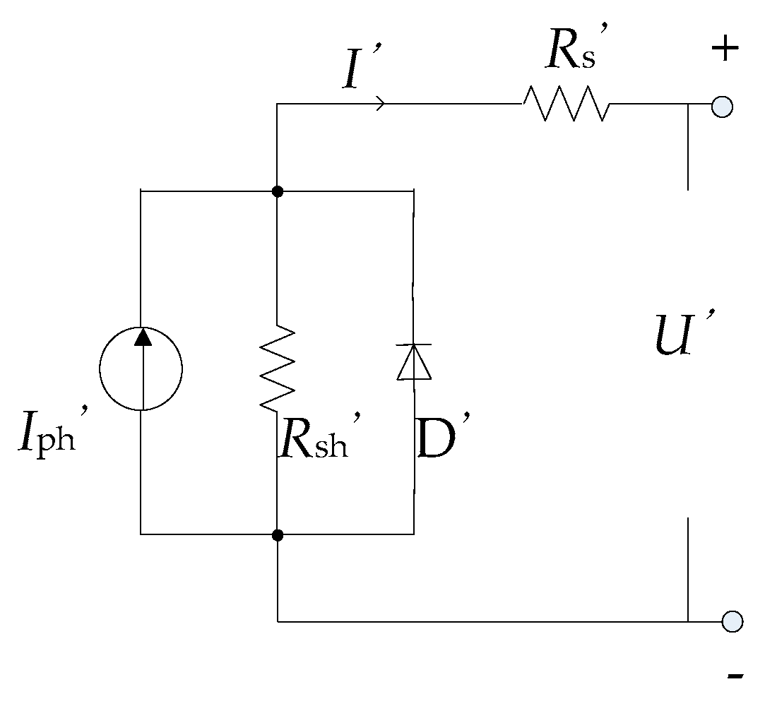
Figure 4.
The V-I curves of the 3 × 2 photovoltaic array in different states.

Figure 5.
The multi-classification diagram. (a) the multi-classification diagram of the training set; (b)the multi-classification diagram of the testing set.
Figure 5.
The multi-classification diagram. (a) the multi-classification diagram of the training set; (b)the multi-classification diagram of the testing set.

Figure 6.
The experimental platform. (a) The experimental photovoltaic system; (b) The experimental instrument. DC: Direct Current.
Figure 6.
The experimental platform. (a) The experimental photovoltaic system; (b) The experimental instrument. DC: Direct Current.

Figure 7.
The classification of test samples.


Table 1.
The parameters of CHN310-72P.
| Parameters | Values |
|---|---|
| Maximum power current Im (A) | 8.36 |
| Maximum power voltage Um (V) | 37.10 |
| Short-circuit current ISC (A) | 8.86 |
| Open-circuit voltage UOC (V) | 44.00 |
Table 2.
The standardization data of the fault features of 10 test sample groups in short-circuits state.
Table 2.
The standardization data of the fault features of 10 test sample groups in short-circuits state.
| The Fault Features | Z1-UOC | Z2-ISC | Z3-Um | Z4-Im | Z5-Iρh | Z6-RS | Z7-Rsh |
|---|---|---|---|---|---|---|---|
| 1# | 0.2137 | 0.6974 | 0.3387 | 0.7831 | 0.6974 | 0.2084 | 0.7831 |
| 2# | 0.2000 | 0.7227 | 0.2837 | 0.7214 | 0.7227 | 0.2376 | 0.7214 |
| 3# | 0.2378 | 0.7139 | 0.3369 | 0.7524 | 0.7139 | 0.2641 | 0.7524 |
| 4# | 0.2819 | 0.6996 | 0.2069 | 0.8000 | 0.6996 | 0.2726 | 0.8000 |
| 5# | 0.2530 | 0.7964 | 0.3101 | 0.7426 | 0.7964 | 0.2758 | 0.7426 |
| 6# | 0.2062 | 0.7618 | 0.2351 | 0.7930 | 0.7618 | 0.2000 | 0.7930 |
| 7# | 0.2578 | 0.8000 | 0.2484 | 0.7643 | 0.8000 | 0.2083 | 0.7643 |
| 8# | 0.2894 | 0.7282 | 0.2000 | 0.7325 | 0.7282 | 0.3166 | 0.7325 |
| 9# | 0.2301 | 0.7970 | 0.3220 | 0.7533 | 0.7970 | 0.2378 | 0.7533 |
| 10# | 0.2297 | 0.6690 | 0.2863 | 0.7868 | 0.6690 | 0.2947 | 0.7868 |
Table 3.
The posteriori probabilities of 10 test sample groups in short-circuit state.
| The Two-Classifiers | 1&2 | 1&3 | 1&4 | 2&3 | 2&4 | 3&4 |
|---|---|---|---|---|---|---|
| 1# | 0.9629 | 0.6045 | 0.5476 | 0.6753 | 0.6773 | 0.6572 |
| 2# | 0.9134 | 0.5660 | 0.5407 | 0.6644 | 0.6328 | 0.6651 |
| 3# | 0.9235 | 0.6057 | 0.5472 | 0.6734 | 0.6735 | 0.6689 |
| 4# | 0.8862 | 0.7007 | 0.5651 | 0.6904 | 0.8952 | 0.7176 |
| 5# | 0.9783 | 0.6160 | 0.5491 | 0.6786 | 0.7073 | 0.6645 |
| 6# | 0.9724 | 0.6364 | 0.5530 | 0.6831 | 0.7266 | 0.7033 |
| 7# | 0.9654 | 0.5867 | 0.5443 | 0.6715 | 0.6625 | 0.6423 |
| 8# | 0.8526 | 0.7227 | 0.5512 | 0.6625 | 0.6534 | 0.6235 |
| 9# | 0.9238 | 0.6808 | 0.5813 | 0.6912 | 0.7913 | 0.6518 |
| 10# | 0.9595 | 0.5775 | 0.5426 | 0.6693 | 0.6505 | 0.6465 |
Table 4.
The final posteriori probabilities of 10 test sample groups in short-circuits state.
| The Fault Types | The Short Circuit | The Open Circuit | The Abnormal Aging | The Normal | The Actual Fault Type | The Fault Type of Diagnose |
|---|---|---|---|---|---|---|
| 1# | 0.4249 | 0.1282 | 0.1614 | 0.2855 | 1 | 1 |
| 2# | 0.3926 | 0.1028 | 0.1780 | 0.3266 | 1 | 1 |
| 3# | 0.3751 | 0.1315 | 0.1931 | 0.3003 | 1 | 1 |
| 4# | 0.3553 | 0.2988 | 0.2049 | 0.1410 | 1 | 1 |
| 5# | 0.4285 | 0.1271 | 0.1631 | 0.2813 | 1 | 1 |
| 6# | 0.4093 | 0.1497 | 0.1593 | 0.2817 | 1 | 1 |
| 7# | 0.4248 | 0.1251 | 0.1812 | 0.2689 | 1 | 1 |
| 8# | 0.3837 | 0.1518 | 0.1625 | 0.3020 | 1 | 1 |
| 9# | 0.4405 | 0.1216 | 0.1478 | 0.2901 | 1 | 1 |
| 10# | 0.4340 | 0.1202 | 0.1516 | 0.2942 | 1 | 1 |
Table 5.
The comparison of three models’ performance. LSSVM: Least Squares Support Vector Machine; SVM: Support Vector Machine.
Table 5.
The comparison of three models’ performance. LSSVM: Least Squares Support Vector Machine; SVM: Support Vector Machine.
| The Fault Diagnose Models | |||||
|---|---|---|---|---|---|
| The LSSVM Algorithm in Bayesian Theory | The LSSVM Algorithm | The Standard SVM Algorithm | |||
| O | Percent | O | Percent | O | Percent |
| 40 | 97.5% | 40 | 92.5% | 40 | 90.0% |
Table 6.
The output probabilities of photovoltaic samples in short-circuits state.
| The Fault Types | The Short Circuit | The Open Circuit | The Abnormal Aging | The Normal | The Actual Fault Type | The Fault Type of Diagnose |
|---|---|---|---|---|---|---|
| 11# | 0.5163 | 0.1237 | 0.1895 | 0.1705 | 1 | 1 |
| 12# | 0.3024 | 0.1303 | 0.4596 | 0.1077 | 1 | 3 |
| 13# | 0.4926 | 0.2902 | 0.1239 | 0.0933 | 1 | 1 |
| 14# | 0.3954 | 0.2197 | 0.2124 | 0.1725 | 1 | 1 |
| 15# | 0.4697 | 0.2303 | 0.1176 | 0.1824 | 1 | 1 |
| 16# | 0.4213 | 0.1478 | 0.1355 | 0.2954 | 1 | 1 |
© 2017 by the authors. Licensee MDPI, Basel, Switzerland. This article is an open access article distributed under the terms and conditions of the Creative Commons Attribution (CC BY) license (http://creativecommons.org/licenses/by/4.0/).
Share and Cite
MDPI and ACS Style
Sun, J.; Sun, F.; Fan, J.; Liang, Y. Fault Diagnosis Model of Photovoltaic Array Based on Least Squares Support Vector Machine in Bayesian Framework. Appl. Sci. 2017, 7, 1199. https://doi.org/10.3390/app7111199
AMA Style
Sun J, Sun F, Fan J, Liang Y. Fault Diagnosis Model of Photovoltaic Array Based on Least Squares Support Vector Machine in Bayesian Framework. Applied Sciences. 2017; 7(11):1199. https://doi.org/10.3390/app7111199
Chicago/Turabian StyleSun, Jiamin, Fengjie Sun, Jieqing Fan, and Yutu Liang. 2017. "Fault Diagnosis Model of Photovoltaic Array Based on Least Squares Support Vector Machine in Bayesian Framework" Applied Sciences 7, no. 11: 1199. https://doi.org/10.3390/app7111199
Note that from the first issue of 2016, this journal uses article numbers instead of page numbers. See further details here.