1. Introduction
Wireless embedded systems or mobile devices in the form of Internet of things (IoT) systems have become ubiquitous in our daily lives. IoT systems, embedded sensors, wildlife monitoring [
1,
2], computing power, and wireless data capabilities, have allowed for more data collection and control of systems with less user interaction [
3,
4,
5]. Battery-powered IoT devices must either rely on a stored charge or harvest energy to continue operation. The operational goal of a battery powered IoT device would be to maintain energy-neutral operation (ENO), where no more energy is spent that can be harvested. Typically, the data collection rate of IoT systems is unrelated to the potential amount of energy harvested. Aggressive sensing may drain the system’s charge by using more energy than can be harvested. Deployed IoT devices, in the form of geo-location solar powered animal behavior monitors, are a candidate for examining the impact of a proportional data collection rate on the stored charge and harvestable energy. Currently, during extended periods where behavior monitor energy consumption may exceed harvesting, the battery can become depleted. The monitor will halt data collection until the battery is fully or mostly charged. Delaying data collection until a full charge avoids oscillating between empty and the minimum threshold to function. During the period of time when a device is waiting for the battery to charge no energy can be spent collecting data, which may lead to days or hours of periods where data cannot be collected.
Conservative fixed data collection rates for animal behavior monitors best address the unpredictable nature of solar energy harvesting by attempting to operate with excess stored energy [
1]. The opposite would be aggressive fix rates that would most certainly drain the battery and be unable to continuously collect data. Either remaining fully charged or running out of energy puts the monitoring device in situations where adjustments to the data collection rate might yield more consistent or high rates of data collection. Also, mostly charged Li-ion batteries (above 80%) have been found to last longer than batteries that are consistently fully charged and drained [
6], which is the operating mode of a fixed collection interval scheme. In order to continually collect data, ENO controllers able to vary data collection rates proportional to the amount of energy harvested were sought for an IoT animal behavior monitoring device.
2. Significance of the Problem
Two major operating schemes were observed from data in a recent study by Miller [
7] of wildlife tracking data due to a fixed rate of data collection of 15 minutes. Firstly, available energy from the battery dropped below a minimum charge level and data collection stopped until adequate energy had been harvested and stored. Secondly, batteries remained mostly or fully charged due to harvested energy being greater than the sensor usage energy. The two cases described are opposites in that there were either data gaps or the data collection rate was consistent. Since both devices were deployed at the same location and the animals migrated to different regions of North America, the performance was clearly tied to the potential for energy harvesting. In addition, had the data collection rates been adjusted to reflect the energy harvesting potential, gaps in data or more data may have been achieved. The devices’ data collection rates were not adjusted during the study, which is something that must occur manually on a remote system. Fixed data collection rates are typical of wildlife behavior devices due to simplicity of operation [
7]. Movement data collected by animal behavior monitors are typically desired at fixed intervals for ease of integration into statistical behavior models, but are rarely achieved due to sometimes aggressive data collection rates.
In addition to the previous study, devices with consistently low Li-ion battery levels have been shown to have significantly shorter life cycles than devices with consistently full batteries and continually charging a Li-ion battery to 100% may reduce the cycle life [
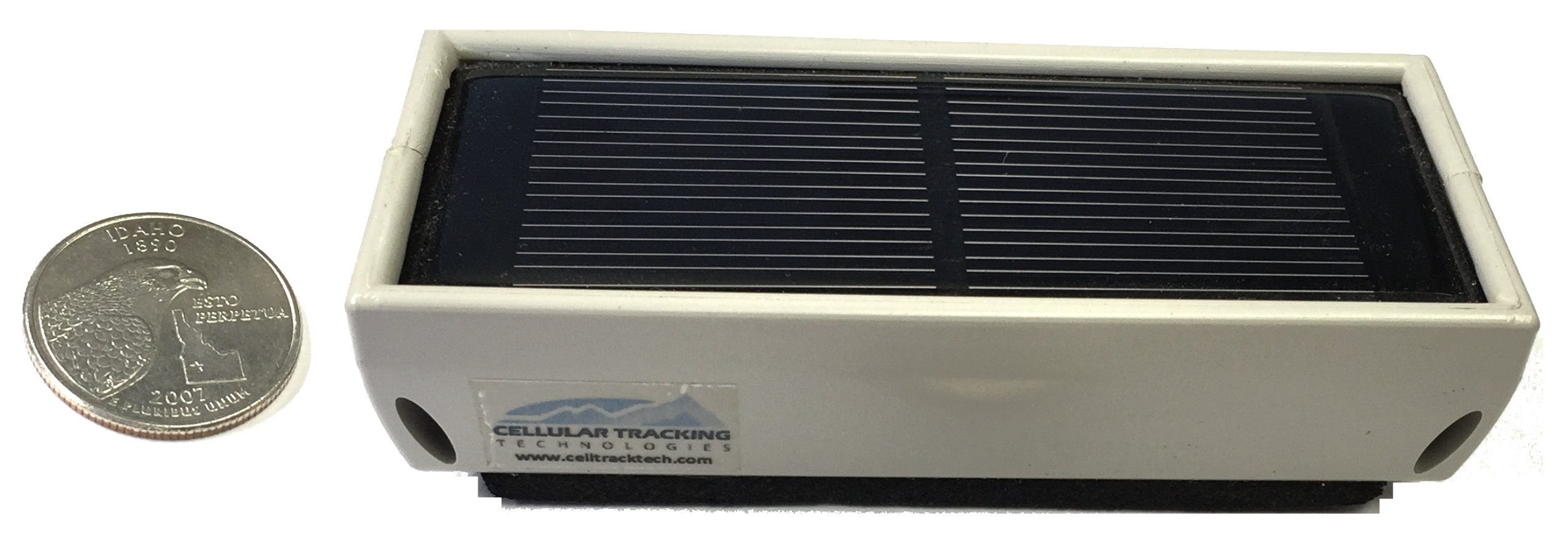
6]. Therefore, maintaining a fully charged battery may not be beneficial to maintaining the operational lifetime of a remotely-deployed wildlife behavior monitor. Energy usage of a wildlife behavior monitoring device manufactured by Cellular Track Technologies (CTT) shown in
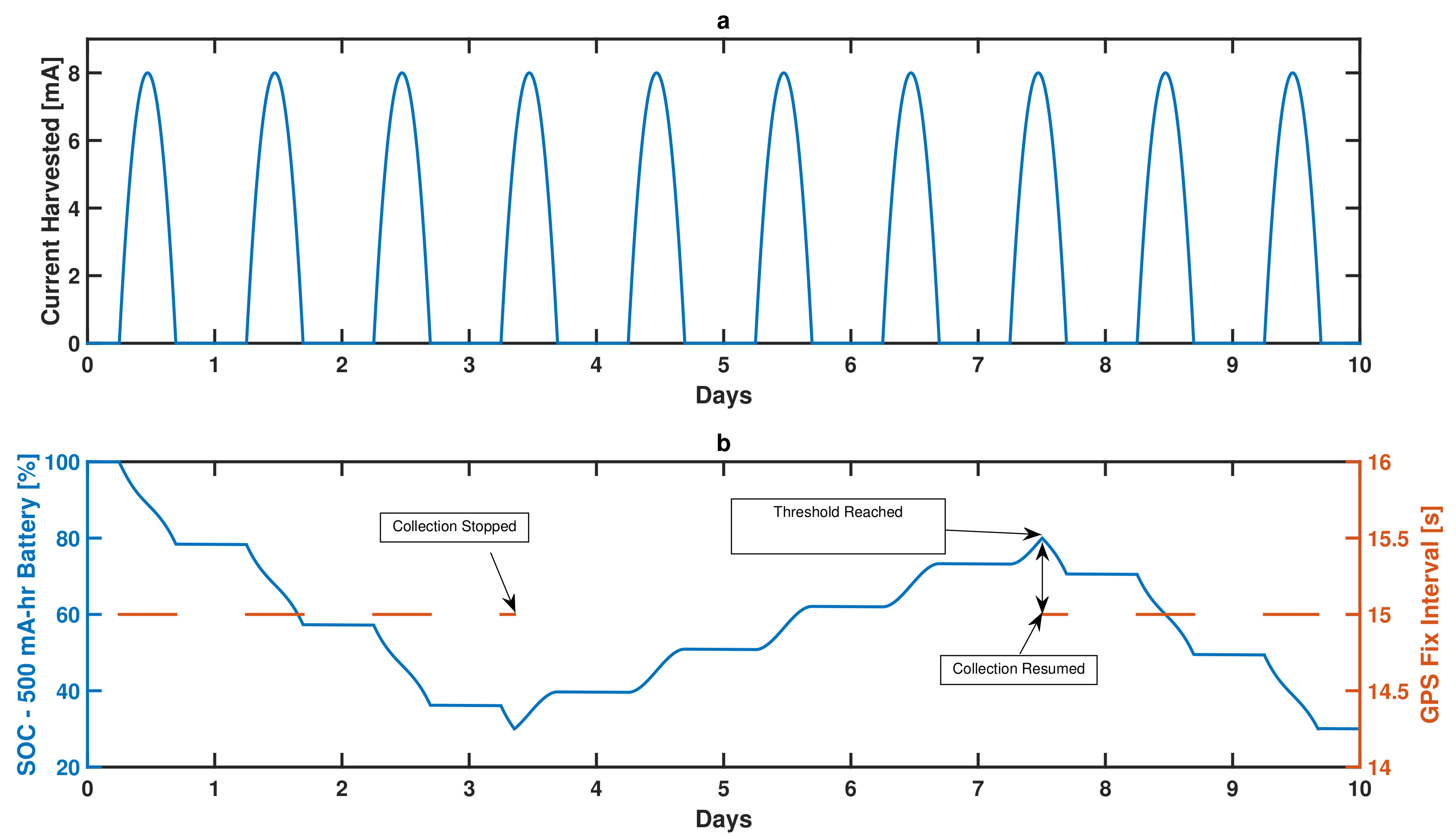
Figure 1, was measured in a fixed setting using a programmable power supply to mimic solar energy in order to illustrate the problem with a fixed data collection rate that exceeds the harvested energy. The selected rate was too aggressive for the amount of harvestable energy (shown in
Figure 2), and data collection had to be stopped after three days to allow a four-day charging cycle. If left alone, the charge and discharge cycle would continue to oscillate, leaving gaps in data collection. Solutions were sought that would automatically adjust a behavior monitor’s data collection rate based on the availability of solar energy such that (1) a fully charged battery (>80% capacity) is maintained and (2) variation in data collection rate is reduced.
3. Related Work
Wildlife behavior monitors can be classified into three basic groups categorized by their data retrieval method: (1) Same-message burst transmitters; (2) data loggers; and (3) data transceivers. These are summarized in
Table 1. In the first group, same-message burst transmitters broadcast an encoded unique number that must be received by one or more base stations within their transmission range [
8,
9] and include Radio Frequency Identification Device (RFID) tags [
10,
11]. RFID tracking devices do not typically transmit any information other than a unique number for identification. For the second group, loggers archive sensor data, but require manual retrieval which can potentially lead to complete data loss [
12]. Both data loggers and same-message transmitters are typically designed for tracking small animals and as a result may not include methods for energy harvesting because overall device size and weight may interfere with natural behavior of the study animal. With respect to the third group, data transceivers typically use GPS satellite localization and transmit acquired data through radio communication [
13]. In addition to functionality, behavior monitoring devices can be classified by their energy needs. In general, burst transmitters typically use the least amount of energy or none in the case of passive RFID, with logging style devices second, and transceivers requiring the highest level of energy. This study selected a data transceiver for analysis and development due to the largest potential impact on performance and because the data collection rate can be regulated to manage energy consumption.
Energy supply is critical to IoT wireless sensor devices, as lifetime and utility of the sensors are based on how long a battery can sustain operation [
4,
14,
15]. Harvesting energy from the environment has to supplement stored battery energy [
16,
17,
18,
19,
20,
21,
22] and selection of processing modes based on available energy [
23] are common methods of extending operating life of IoT devices. Photovoltaic cells (PVC) can be used for solar energy harvesting and provide a renewable energy resource that is well suited for behavior monitors [
11,
24]. However, any freely available energy source many have uncertainty in its delivery. Solar capture systems may be impacted by factors such as the solar diurnal cycle, weather patterns, and shading from foliage [
25,
26]. Several behavior monitors have been created that utilize energy harvesting, but they typically collect data, and consequently spend energy, at conservative fixed intervals [
27,
28]. In addition to harvesting energy from the environment, responsible spending of energy for data collection must occur so as to not prematurely use all stored energy.
Scheduling and prioritization of tasks or sensor data collection is known to extend device operation by selectively performing tasks based on a threshold of available energy, or task energy cost. As a result, device energy consumption can effectively be reduced while still remaining partially operational [
29]. This method may be unable to adjust energy consumption rates to with a variable acquisition time sensor such as GPS. The use of a hard threshold is the major issue with commonly used energy reduction techniques. In addition, when not collecting data, a system should take careful consideration proper methods of reducing power consumption of the system as a whole and in particular the microcontroller. The exact reasons for sleep at appropriate states or scale-back operation of a microcontroller can have profound long-term impacts on power usage [
30]. In practice, harvested energy is never consistent. This is especially true for migratory animals, meaning that an energy-harvesting behavior monitor must adapt its energy consumption relative to its harvesting rate. The energy consumption of a wildlife behavior monitor is not consistent enough to model with traditional linear techniques due to the variation in acquisition time for sensors such as the GPS. Achieving Energy Neutral Operation (ENO) for an animal behavior monitoring device has typically first required modeling of the energy consumption and harvesting [
31], then development of a sensor rate control system. An energy usage model of wireless sensors nodes was developed by [
24] that was used to develop an adjustable solar data collection rate to achieve ENO. Solar energy was assumed to be periodic and proportional to a diurnal cycle. In the model presented in [
24], a period of 24 h was broken into blocks and a constant value for incoming energy was assigned to each block. Data collection was then modified based on a difference in measured and predicted energy for each of these blocks. Any deviation from predicted and actual energy harvested may result in sub-optimal data collection due to periods of depleted or full battery charge. Vigorito presented a model-free, adaptive control algorithm that modified data collection to meet the following metrics: ENO, performance maximization, and duty cycle stability [
32]. Selecting a data collection rate that balanced energy consumed and harvested was developed using linear-quadratic tracking to minimize the difference between battery charge and a target value. These techniques were tested with a small set of data on a constant energy consuming sensor. Their results indicated that highly variable harvesting rates, which have been seen on wildlife tracking devices, may be an issue when using their algorithm. Computational impact of a control method for ENO should be of concern and the most functional and minimal algorithm should be selected. There are many options for feedback control algorithms that may achieve intended research goals, and several of the most popular ones were compared regarding computational impact. Fuzzy logic is a method of using linguistic expressions and activation functions to form a control value. The linear quadratic regulator (LQR) is an optimal control method that minimizes the cost function and requires calculation of a gain matrix before use. Proportional–integral–derivative (PID) control is a simple method that relies on three gain values that can be tuned automatically given a linear model or manually. PID control was used by [
33] to adjust data collection such that an energy storage element was maintained at a constant level. State of charge (SOC) was used as a control signal and the node duty cycle was manipulated.
is a non-linear optimal method of control that normally guarantees robust performance of systems. Several studies [
34,
35,
36] have compared computational and control performance of PID, LQR,
, and fuzzy logic using an servo and inverted pendulum on embedded resource-limited systems and found that PID was able to achieve similar goals as the other methods and required about 3% of the execution time and memory resources compared to the most complicated, fuzzy logic.
Overall, published research indicated that in order to achieve ENO, a controller specific to the device could be developed using various classical control techniques based on an energy consumption model. Energy-harvesting behavior monitors have potential for indefinite life if the collection rate is able to adapt to the rate of harvest-able energy, maintaining ENO. Several methods were suggested in literature, mainly for short timespan (<1 s) operation given some harvested energy. Wildlife behavior mounting devices are typically deployed for years at a time, can collect tens of thousands of position fixes, and may experience large time periods (months) where little energy can be harvested. The specific needs of behavior monitors, long times of deployed operation, and ability to adjust operation given highly random energy harvesting required investigation into application of specific methods that would lead to ENO.
4. Energy Consumption Model
Analysis and development of a controller to maintain ENO of a behavior monitor required an energy consumption and harvesting simulation model representing a typical tracking device. The CTT-1000a series, shown in
Figure 1, is a 40 mm × 100 mm × 21 mm wildlife behavior monitor weighing 70 g that was selected for analysis and modeling to develop an ENO controller. Each of the tracking device’s energy consuming and harvesting components were broken down in a systematic fashion for modeling and then compared to a fielded CTT-1000a deployed on Golden Eagles in eastern North America. The particular set of data used for validation was chosen because the actual deployed devices experienced a wide variance of harvesting energy and would benefit from a controlled rate. The CTT-1000a wildlife behavior monitor consists of an MSP430 microcontroller, a GPS receiver, a real-time clock, FLASH data storage, a Li-ion battery, a Global System for Mobile Communications (GSM) cellular modem, and solar panel tightly integrated into a single system.
Measurements of the energy and power usage for each component of the CTT-1000a were performed by using a fixed voltage DC power supply and a high-accuracy digital multimeter (Tektronix DMM-4020). Several of the components included voltage regulators to satisfy input requirements. Therefore, measurements instead of manufacturer-stated current draws were used to gain a more accurate model of the system rather than just the individual components such as only the GPS module. In addition, due to each component utilizing a regulator to produce lower voltages than the battery, current draw to each component was independent of the battery voltage. Therefore, current draw can be used as the main indicator of power consumed and represents a direct translation to battery capacity used without having to consider power.
The tracking device selected for modeling contains the ability to individually toggle power to components using the on-board microcontroller. Initially, the microcontroller’s power consumption was measured in active and sleep mode. Next, each of the other system components were toggled on separately where the microcontroller’s active current usage was subtracted out of the measured value since components could not be isolated, as shown in
Table 2. All measurements were taken using a DC source set at Li-ion batteries with a nominal voltage of 3.7 V. The component measurement along with operation time allows for an insight of how much total energy would be required for a period of operation. For example: during a 24-h period, there are typically 60 GPS fixes collected that take about 1 min and one cellular modem operation, that to send 60 fixes, takes 2 min. The component usage information is able to assist a designer with an energy impact in that if no energy is harvested, 28
of cellular modem would be used during a day. The modem device was a Telit-865 quad band GSM cellular network node. Taking into account the microcontroller operating during the GPS and modem periods, as well as sleep usage, 185
of battery is used. Therefore, to last at least one day using a configuration of 15-min GPS fixes at 60 per day with one cellular operation, a 241
battery is required.
4.1. Model Design
Each component of the behavior monitoring device was represented using a function that kept track of the components power state, used the current time as input, and delivered the amount of energy consumed since the last time step. Software modeling of the selected behavior monitor was implemented using MATLAB. At each time step, current of each components’ current consumption was summated and then converted to milliampere-hours using the amount of time between samples. After all of the component’s energy usage were summated for the time step, any excess current available from the PVC was then directed to the battery model to simulate charging. The components included for power usage modeling included the microcontroller, GPS, the cellular modem, the photovoltaic cell, and the battery. Components such as the flash memory and real-time clock were included in the microcontroller model.
4.2. GPS
Typical GPS receivers are capable of a low-power sleep where ephemeris data is held in memory for a hot start, which in some situations (short durations between fix requests), may provide position data faster with less energy required than a cold start. A GPS receiver was modeled using three states of operation: (1) Active, where the receiver was fully powered and seeking or tracking a position; (2) Sleep, where the receiver was holding information in memory and checking its position periodically as configured by the manufacturer; and (3) Off, where no power was being used by the receiver. The active mode was modeled with a current draw of 27.5 mA while a fix was being acquired, which takes 45 s from power on (cold start) or 5 s coming out of sleep (hot start). Sleep mode was measured to be 441 A and occurred between requested fixes. Off mode corresponded to 0 mA.
Time to First Fix (TTFF) was modeled by relating to the GPS receiver’s operational state (Active, Sleep, or Off) and the required minimum position acquisition time. While Active, the acquisition time was considered to be 1 s. During Sleep, the acquisition time was 10 s. Transition from the Off state to acquire a position required 45 s.
Selection of which GPS operational state to use for minimal power usage required a simple analysis of the states. Fix intervals less than or equal to 10 s utilized the Active state. In between 10 s and 15 min fix intervals, the GPS was placed into Sleep state in between acquisitions to time and the power required over a full startup from an Off state. Any requested fix interval greater than 15 min places the GPS receiver in an Off state in between location acquisitions.
4.3. Photovoltaic Cell
Energy harvesting was achieved by using a photovoltaic cell (PVC) that converts light radiation into electrical energy. The CTT-1000a contains an 80 mm × 40 mm panel with a nominal 5 V, 150 mA source. Sourced current from the PVC was modeled using a second-order polynomial curve fit, of the form
, where the coefficients were found by analyzing a moving average of 31 days of PVC current data from a field-deployed CTT-1000a tracking device. Empirical data averages of 10.5 h for sunlight duration, and a maximum current draw of 10 mA, were used with the MATLAB function polyfit to generate coefficients for
a,
b, and
c. Equation (
1) shows modeled current-generated
based on 10.5 h day using the values of sunrise at 6:00 a.m., sunset at 16:30 p.m., and a maximum current draw of 10 mA. The PVC model included the ability to adjust noise for simulation of intermittent cloud cover or activity outside of direct sunlight and maximum intensity for different seasons and parts of the world.
A noise component similar to the device used in [
7] of the sourced PVC current was introduced to model factors such as cloud cover, partial PVC obstruction, or lack of sunlight due to foliage. Equation (
2) shows noise current
, between a lower
and upper
bound, where these limits represent
of
from Equation (
1), which is similar to literature describing modeling of energy-harvesting PVCs [
37].
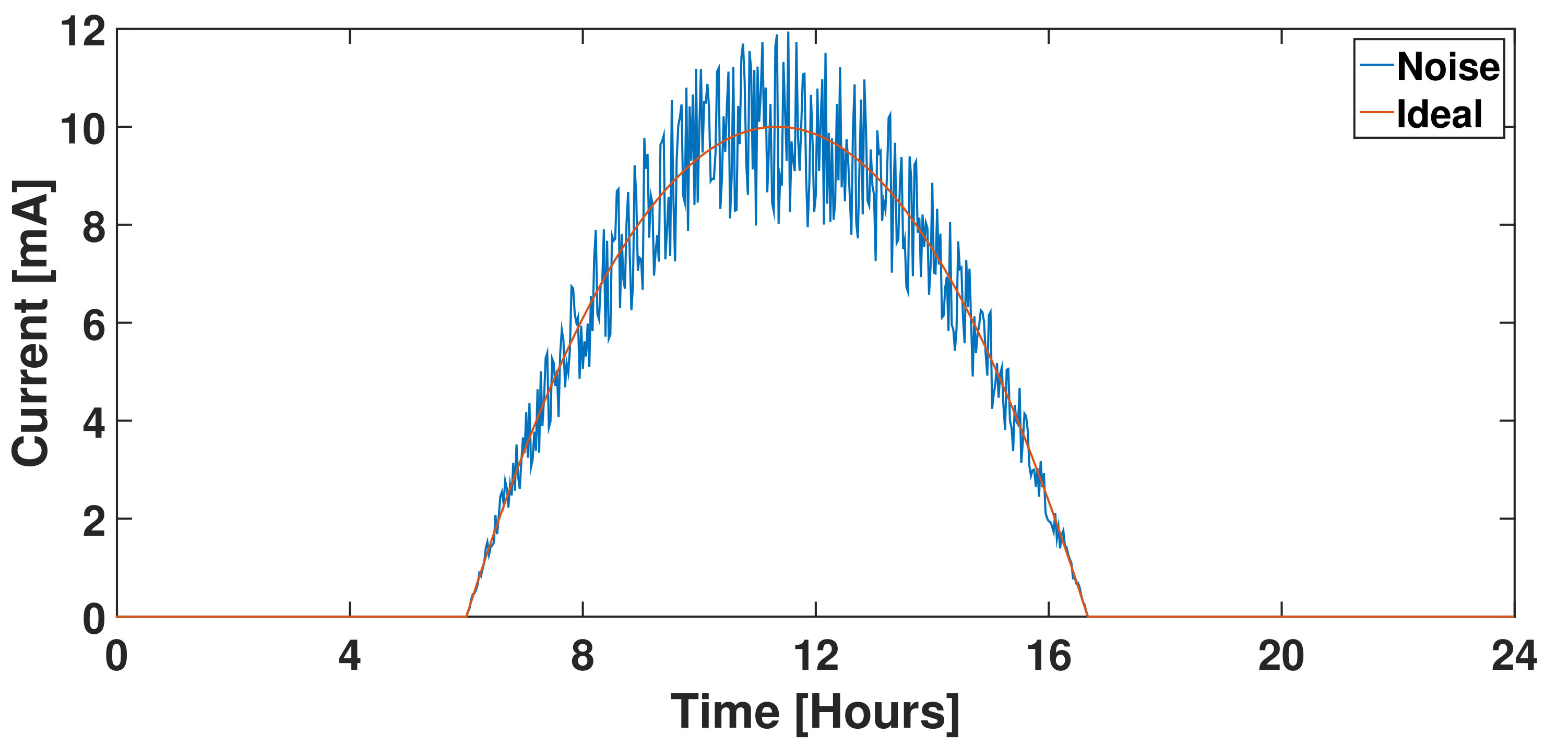
PVC current generation was modeled for a period of 24 h at a time step of 1 s as seen in
Figure 3 to examine energy harvesting in detail for a single day. Energy harvested by the model was zero outside of daylight hours.
4.4. Battery
The battery of a behavior monitoring device was modeled as a container with a minimum and maximum level of store-able energy (
) and efficiency of charge. Battery level could not exceed the maximum value, and was considered completely discharged at the minimum value to avoid damage to the battery. The maximum capacity was selected as 800
(fully charged) and the minimum as 10
(fully drained). Net current draw from modeled components was converted to
, for each time step, then added or subtracted from the battery. Battery state of charge (
), defined as the ratio between present battery level
(
) and maximum battery capacity
(
), was used to represent available battery energy. SOC was updated at each time step
by dividing the net current entering or leaving the system
, then adding it to the previous value
(See Equation (
3)). For the occurrence of the first calculation of SOC, the battery was assumed to be fully charged, therefore having an initial SOC of 100%.
4.5. Energy Consumption Model Validation
The objective of creating an energy consumption model was for use as a tool in developing and testing a variable data collection rate system. Before design or performance testing, the degree to which an energy consumption model represented a wildlife behavior monitor needed to be validated.
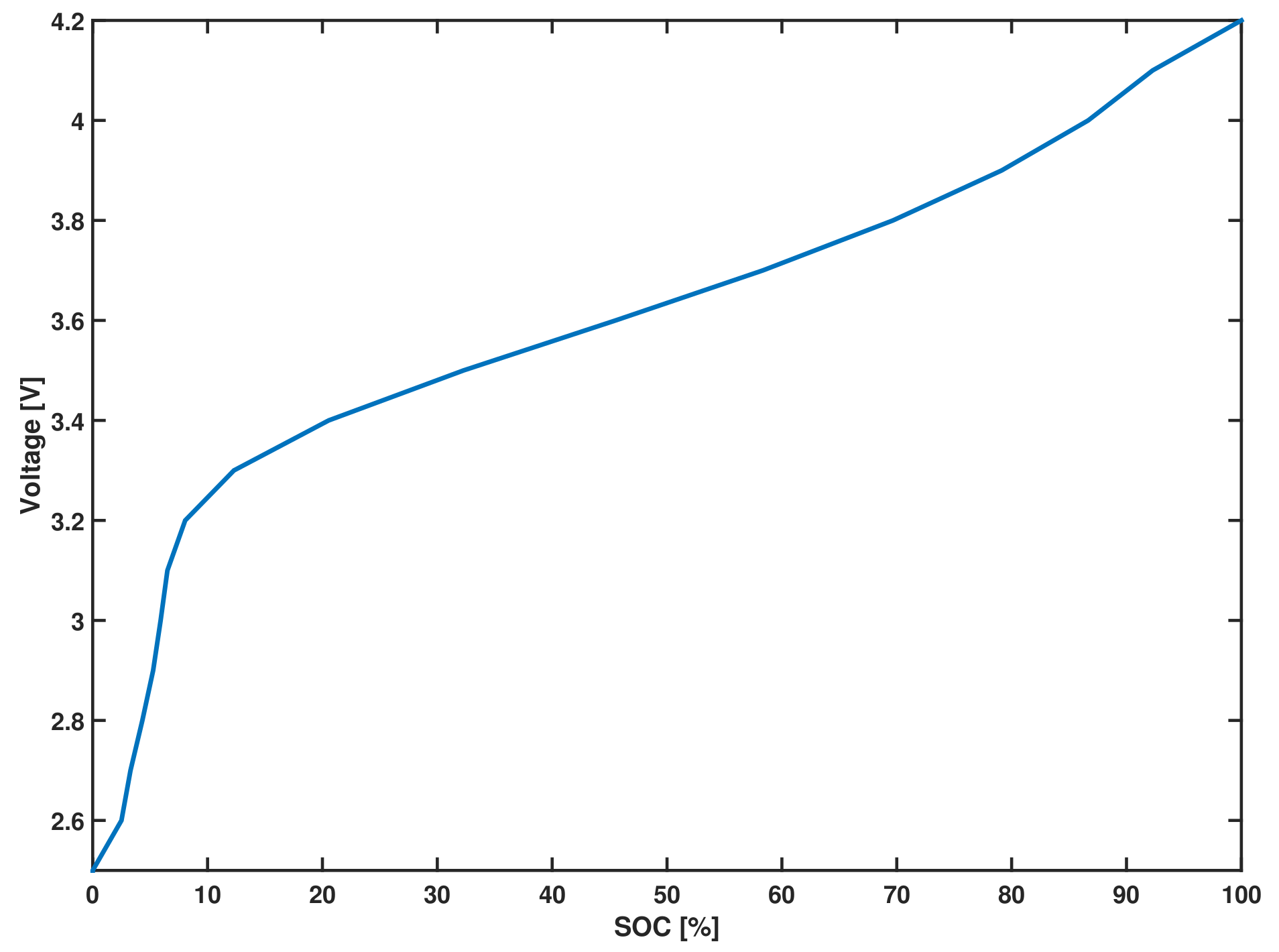
Validation of the developed wildlife behavior monitor tracking device model was performed by matching operating parameters for the energy consumption model to empirical data acquired from a CTT-1000a wildlife telemetry device. Real fix rate and battery performance data were collected from a field-deployed behavior monitoring device on a golden eagle free-roaming in eastern North America [
7]. The fix interval, battery capacity, PVC voltage, and charge rate (mA) measured at each fix acquisition were analyzed. The initial and continuous battery level in terms of SOC were unknown factors and estimations were made using battery voltage. In order to estimate the battery SOC, a direct relationship of voltage and SOC for a Li-ion battery was developed at known load values using the exact same battery model and capacity as the deployed device. For this particular case, voltage of the battery for a 0.01 C was used as the reference load. In order to develop the relationship, measurements were collected of several 800
batteries of the same type as deployed units. First, A Vencon UBA5 battery tester was used to characterize voltage vs. capacity for the 0.01 C load. Next, the collected curves were averaged together, shown in
Figure 4. Finally, linear regression was used resulting in available battery SOC vs. voltage. The particular battery tested was represented by a rational polynomial curve (see Equation (
4)) where the polynomial coefficients are represented in
Table 3.
Measured performance data was compared to the developed energy model by using the following configuration: (1) Solar current generated was linearly interpolated from a rate of 15 min to 1 s to match the model sample period; (2) the fix interval for the model’s GPS data collection rate was set to 15 min; (3) the modeled battery capacity was set to 800
, and the initial battery SOC was determined by the initial deployed device voltage to Equation (
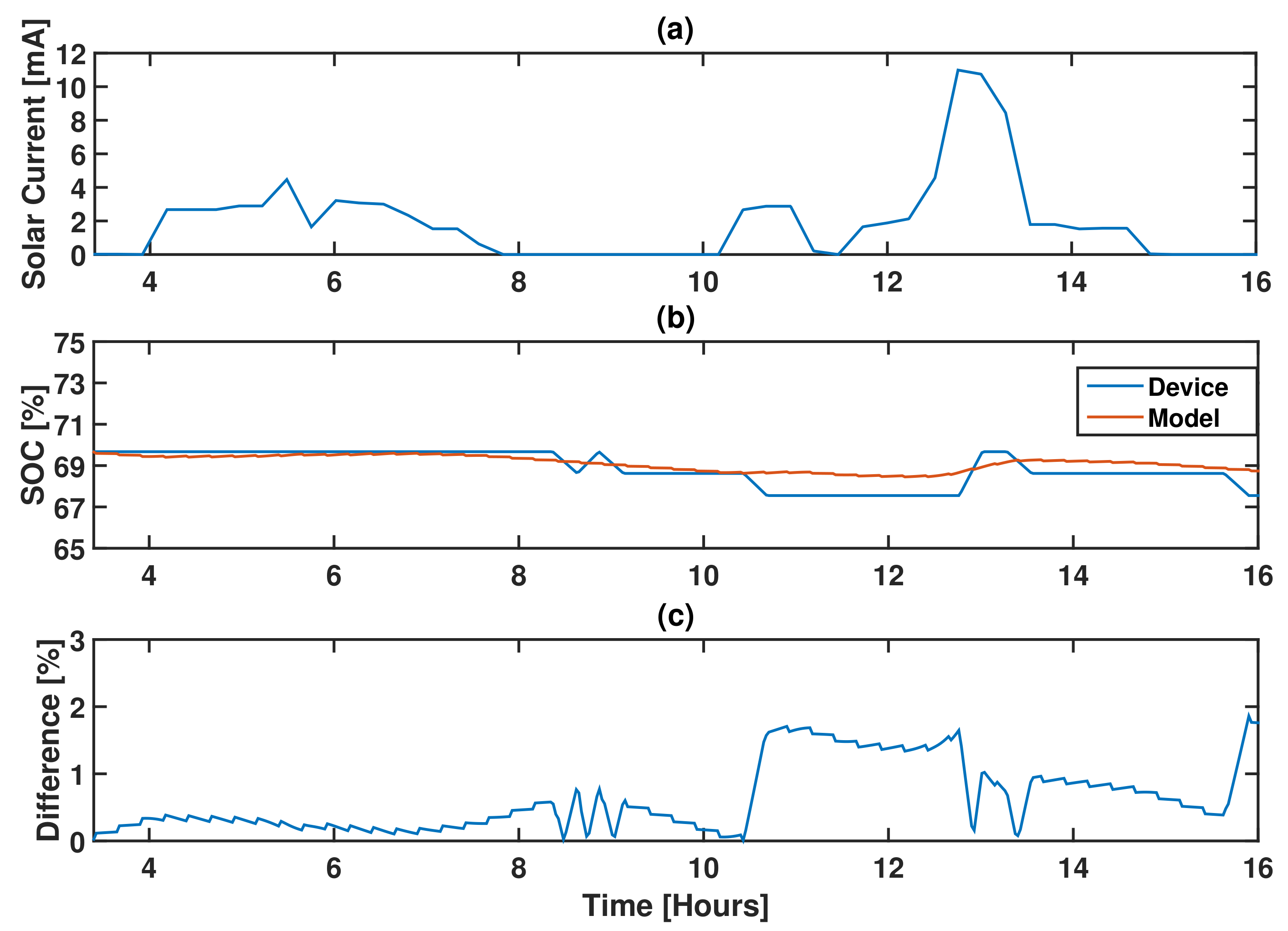
4); and (4) the simulation duration was configured based on the length of time between the first and last data record for each day. Absolute difference between simulated and empirical battery SOC was calculated for each of the 31 days in January 2015 for two behavior monitors. A single day of the device’s solar current and SOC were compared with the developed simulation model and shown in
Figure 5, where (A) represents the actual PVC data from golden eagles in eastern North America [
7], (B) shows the SOC for the device and the models determination of SOC using the PVC data from the device, and (C) shows the difference in the SOC between the model and actual device. Statistical comparisons of the minimum, maximum, and average difference between the model and device data, shown in
Table 4, indicate that the model is capable of generating comparable SOC estimations as an actual device given PVC charge rates.
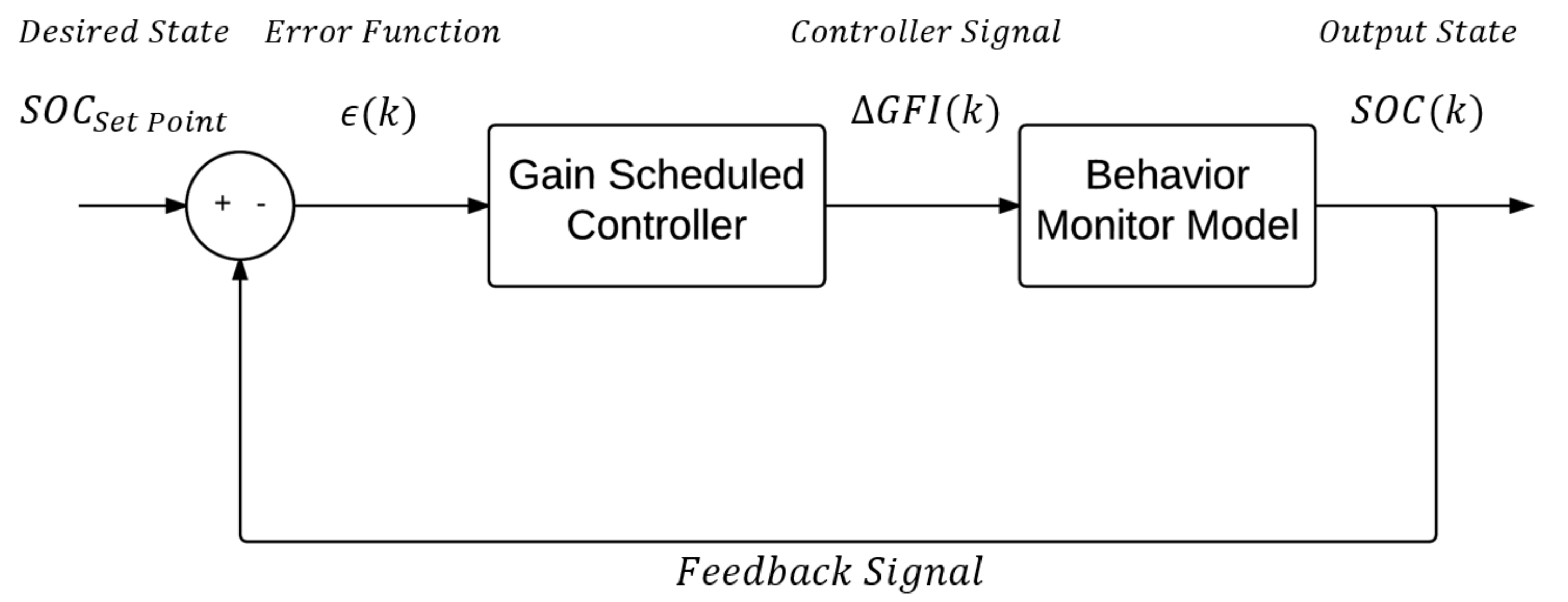
5. ENO Controller Design
The validated energy consumption model of the CTT-1000a was used to design and test a controller with two goals. First, the battery SOC should be maintained at 80% for optimum life according to [
6]. Second, collection rate should be constant or only change in short (once per day) increments. The two design goals needed a scheme that would feed back to the SOC, compare it against a set-point, and then calculate a change in the fix rate, if needed. There are many known control methods that may not have been specifically designed to maintain ENO for the investigated system, such as artificial intelligence [
38], adaptive control [
32,
39], LQR, non-linear control, and feedback control [
40]. The various control methods found were compared for processing execution based on complexity of integration. Feedback control in the form of PID was found the be the simplest, yet was capable of successfully controlling the modeled wildlife sensor system, shown for ENO in
Figure 6. It should be noted that PID is known to work for linear time-invariant systems and the model being used here is a time-varying non-linear system, meaning that extra precautions need to be implemented to avoid output oscillations and asymptotes. The ENO controller developed uses the difference between the desired or set point SOC and the measured SOC to suggest an increase or decrease in the GPS fix interval. At initialization of the system, the GPS fix interval is selected based on predicted knowledge of the device’s location. During operation, the controller is given calculation time after each data collection interval (in this case the GPS fix interval). The controller is then able to increase or decrease the collection interval in order to utilize more available energy or decrease to save energy. The controller consisted of a gain scheduled PID with two sets, upper/lower boundary control, and asymptote detection for a reset. Gain scheduling was done to allow fast adjustments with large errors and very small reactions once the error or desired set point was reached. Typical automated or deterministic PID parameter tuning methods do not work for the developed model due to the non-linearity. Therefore, trial and error simulations using the model will determine the PID gain values and schedule points.
5.1. Controller Gain Tuning
P, I, and D gains for the gain scheduled ENO controller were tuned by a three stage trial-and-error process. Firstly, an initial set of gains were selected based on a constant PVC model of 10 to simplify tuning. Battery capacity was initially modeled as 100 such that impact of energy harvested and consumed on battery level could be correlated to changing gain values. Secondly, adjustments were then made to the initial set of gains to account for replacing a constant-valued PVC model with one dependent on a Sun cycle. Thirdly and finally, a second set of gains, selectable by a gain scheduler, were introduced to reduce fluctuation in data collection rate when battery SOC was within of a set point. Battery information from a CTT proprietary database shows that tracking device life is typically increased when battery levels are consistently high, and therefore a set point of 80% SOC was selected. In addition, battery capacity was selected to be 800 (typically used to power the CTT-1000a) while tuning the second set of gains.
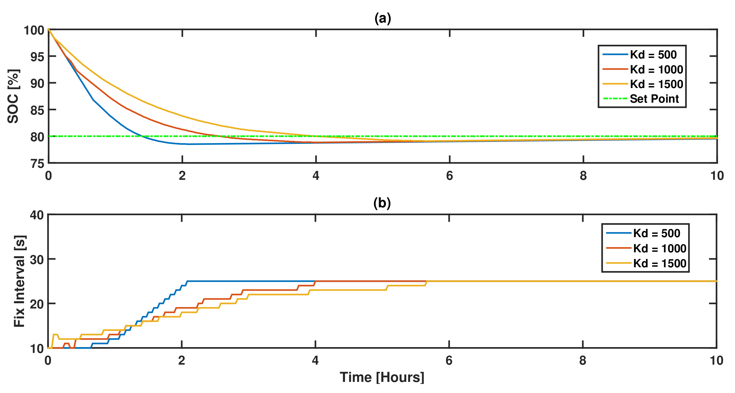
Derivative gain was initially tuned given a previously selected
of 0.3 and
was 0. Battery SOC and GPS fix intervals were evaluated at
values of 500, 1000, and 2000 and, as seen in plot (a) of
Figure 7, SOC had an overshoot of 3%, 2%, and 1% with times to reach an 80% reference point of 2, 4, and 5 h, respectively. Plot (b) shows a GPS fix interval of 25 s was reached in 6, 4, and 2 h for
values of 500, 1000, and 2000, respectively. In summary, a
value of 500 was selected because it had the shortest rise/steady state time of 2 h for the GPS fix interval.
Values for an initial set of PID gains were selected manually, given a constant 10 mA PVC model and a 100
battery capacity.
,
, and
were tuned one at a time by evaluating both battery SOC and GPS fix interval.
was assigned a value of 0.3,
was assigned 2000, and
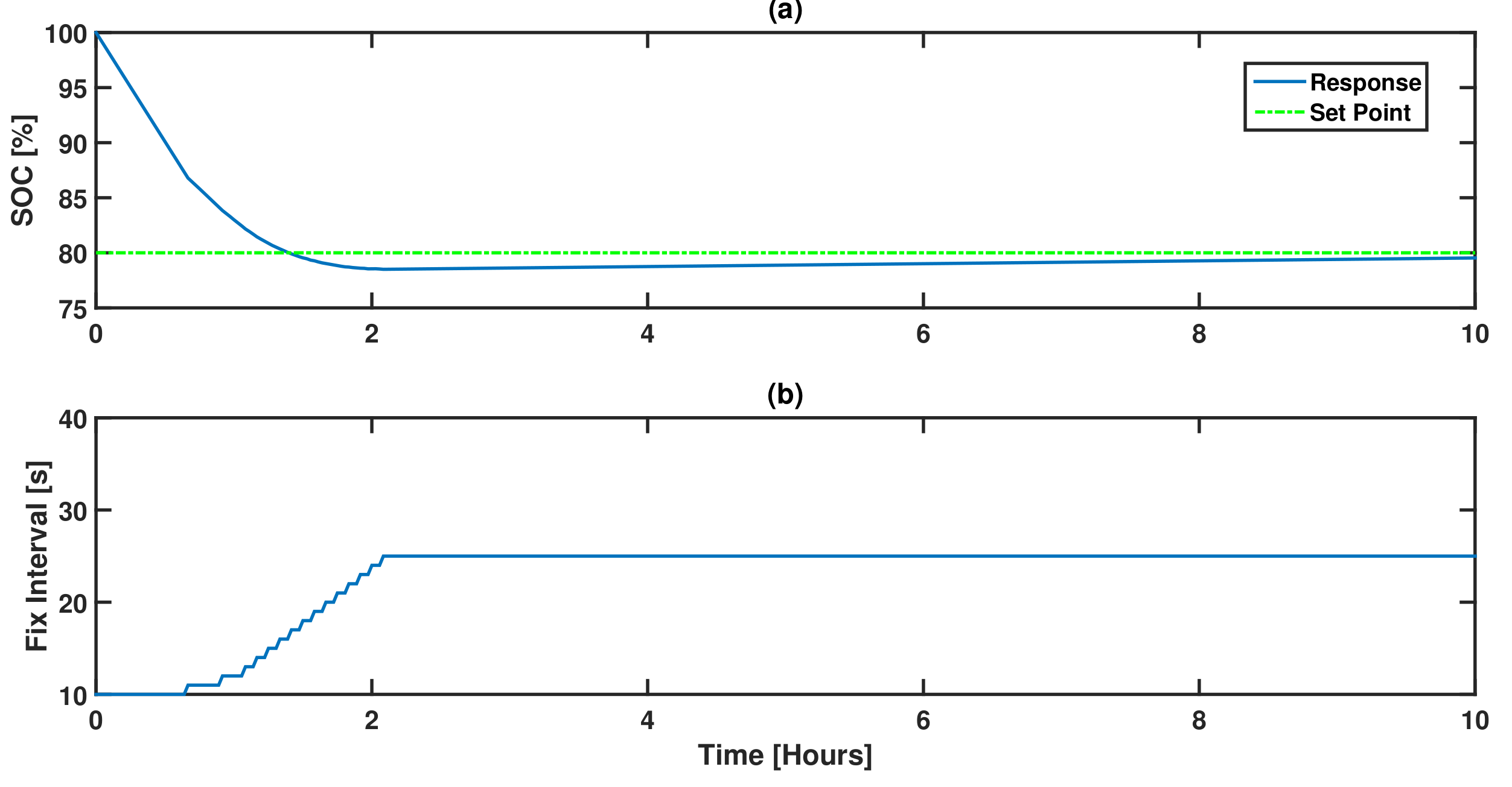
was not used. Plot (a) of
Figure 8 shows simulation results for SOC that started at 100% SOC and reached a reference SOC point of 80% in one hour. GPS fix interval reached a steady state of 25 s in 2 h but SOC did not reach a steady state due to the GPS fix interval being restricted to integer values, where the value needed to achieve SOC steady state was between 24 and 25 s.
5.1.1. Variable PVC Model
The second major step of tuning was performed using a PVC model that varied based on a solar diurnal cycle that included standard noise. GPS fixes were acquired during the day, which was dictated by the PVC model. Battery capacity remained at 100 from the previous tuning step. was re-evaluated for values of 500, 1000, and 2000 respectively. A value of 2000 was selected because GPS fix interval and SOC had the smallest amplitude of oscillation.
Reducing fluctuation in data collection rate near the SOC set point was handled by an additional set of gains, where selection of which gain set to use was determined by a gain scheduler. Tuning of the gains were performed by first setting gain values for data collection consistency (
,
, and
) equal to the first
,
, and
. Simulations were performed for 30 days, battery capacity was 800
, and the PVC model was variable. Plot (c) of
Figure 9 shows GPS fix interval for
evaluated at 1000, 1500, and 2000, where
was previously selected as 0.1.
GPS fix interval settled to 38 s after 28 days for assigned to 1000. Similarly, a GPS fix interval of 38 s was achieved after 22 days for set to 1500. Gain values of both 1000 and 1500 had GPS fix interval variation between 30 to 60 s prior to reaching a steady value. Ultimately the original value of 2000 was selected for , the same value as , because a steady GPS fix interval was achieved in 6 days compared to 22 and 28 days for gain values of 1000 and 1500.
5.1.2. Controller Gain
Controller gain tuning was performed by observation of GPS fix interval and battery SOC. , , and parameters were tuned manually, where one gain parameter was tuned at a time. Two sets of PID gains were used, one for battery SOC to a set point, and another for reducing fluctuation in data collection rate once the set point was reached. Initial values for the first set of gains were selected based on a constant PVC model of 10 mA: was 0.3, was 500, and 0 because the SOC and GPS fix intervals became unstable for non-zero gain values. Additional tuning was performed on the first set of gains after battery capacity was increased from 100 to 800 and a variable PVC model was implemented. was assigned a value of 0.3 and was 2000.
Values for the second set of PID gains were selected to account for fluctuation in GPS fix interval caused by a variable PVC model.
was assigned a value of 0.1,
was assigned 2000, and
was 0.
Table 5 shows the results from tuning for a gain scheduled system. The first set of gains minimized variation in GPS fix interval, and the other drove battery SOC to a reference point. Gain values denoted with a subscript of 1 refer to the gains used for
greater than 10%, and a subscript of 2 represents gain values used that corresponding to
less than 10%.
6. Performance Evaluation
Although solar radiation recurs in a pattern every 24 h on Earth, factors such as weather changes, time of year, or PVC obstruction may cause changes in the amount of energy harvested each day. Performance of the developed controller to maintain a SOC by adjusting the fix rate was investigated compared to the current method of a fixed collection rate. Controller simulations were carried out to determine controller performance of stable fix rate and set point SOC tracking for constant and variable PVC levels. The initial SOC, battery capacity, SOC set point, and PID gains were the same for each simulation. First, the PVC randomness model was used and the controller system was allowed to find a stable fix interval to ensure that the developed controller could arrive at a stable solution. Next, a peak PVC level of 10 or 5 was chosen as a starting point and then changed, respectively to either higher or lower values, once a stable fix interval and SOC was detected. Changing the PVC level was done to simulate a distinct change in climate, location, or nesting either into the condition or away to normal sun exposure.
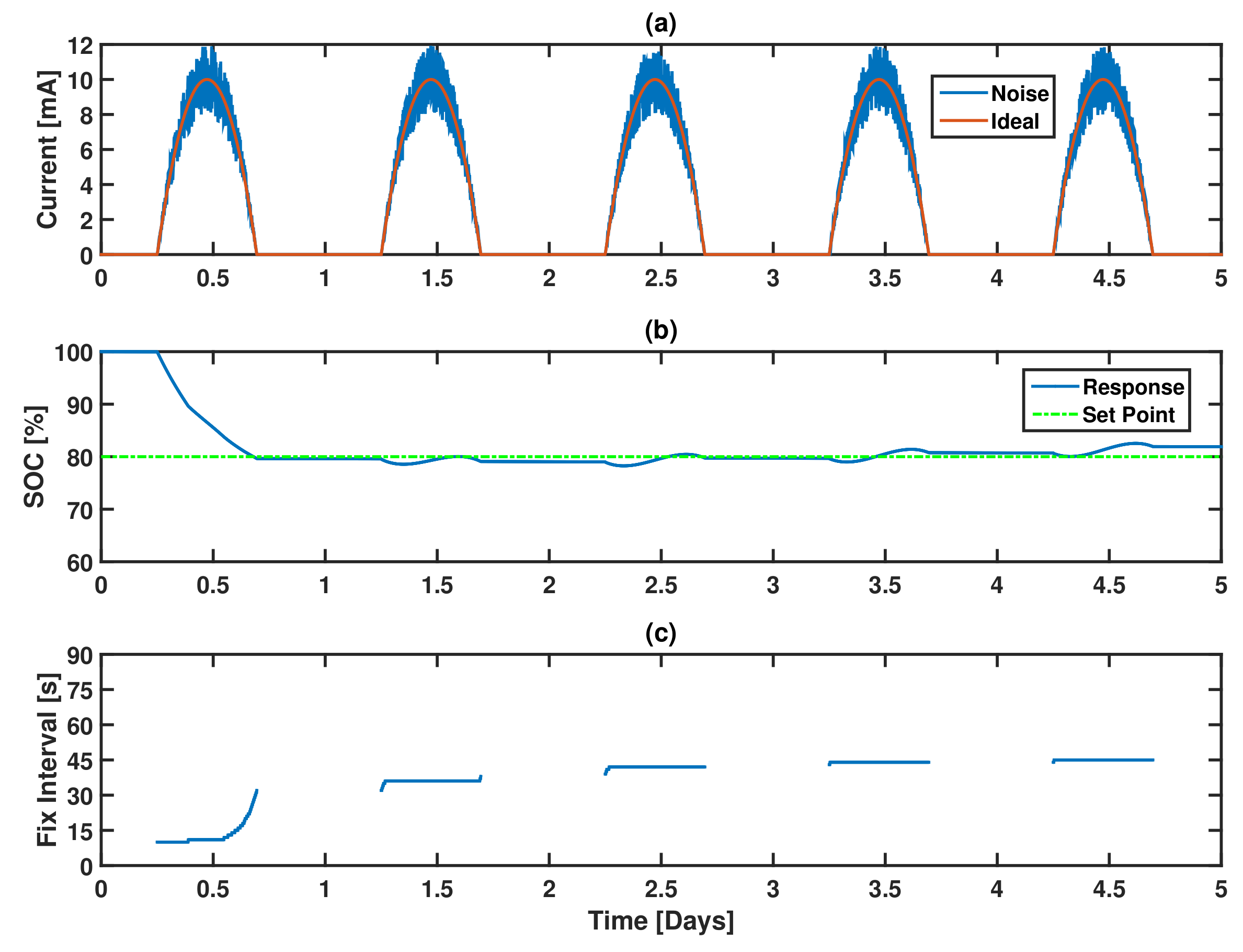
Fixed PVC simulations indicated that for the given configuration (50
battery, SOC starting at 100%, initial fix rate of 5 per minute, only collecting fixes during the day) it took 4 days of operation to reach a constant fix interval. During the first day, there was a steep increase in the fix interval using the first set of gains. The second set of gains then took over and slowly adjusted the fix rate to 45-min intervals. The PVC with randomness, SOC, and fix interval are shown in
Figure 10 for a five day interval. A GPS fix interval increase of 1–3 s was observed at the beginning of each day. This was caused by a controller adjustment due to a decline in SOC as a result of energy consumed from sleeping overnight.
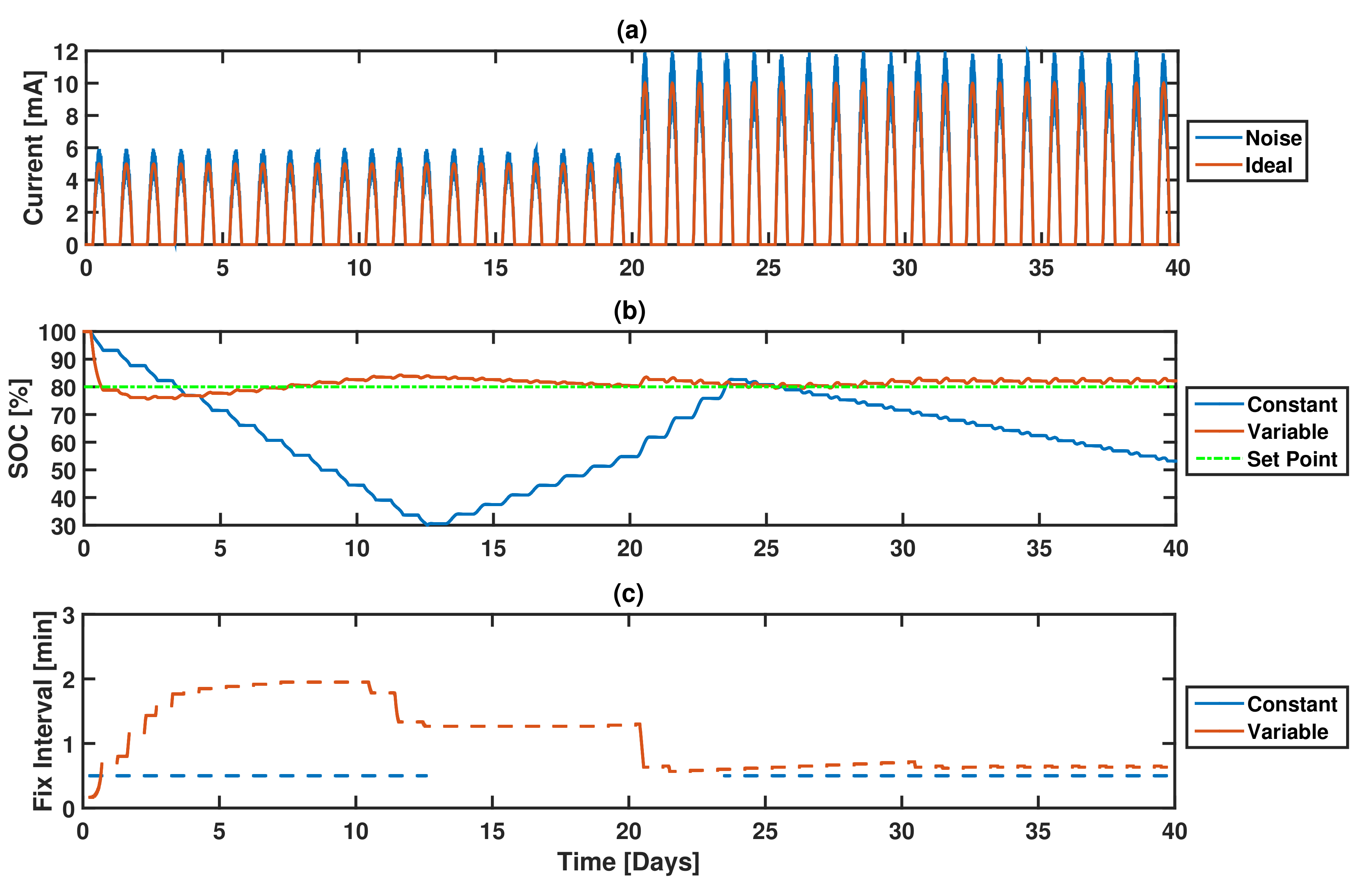
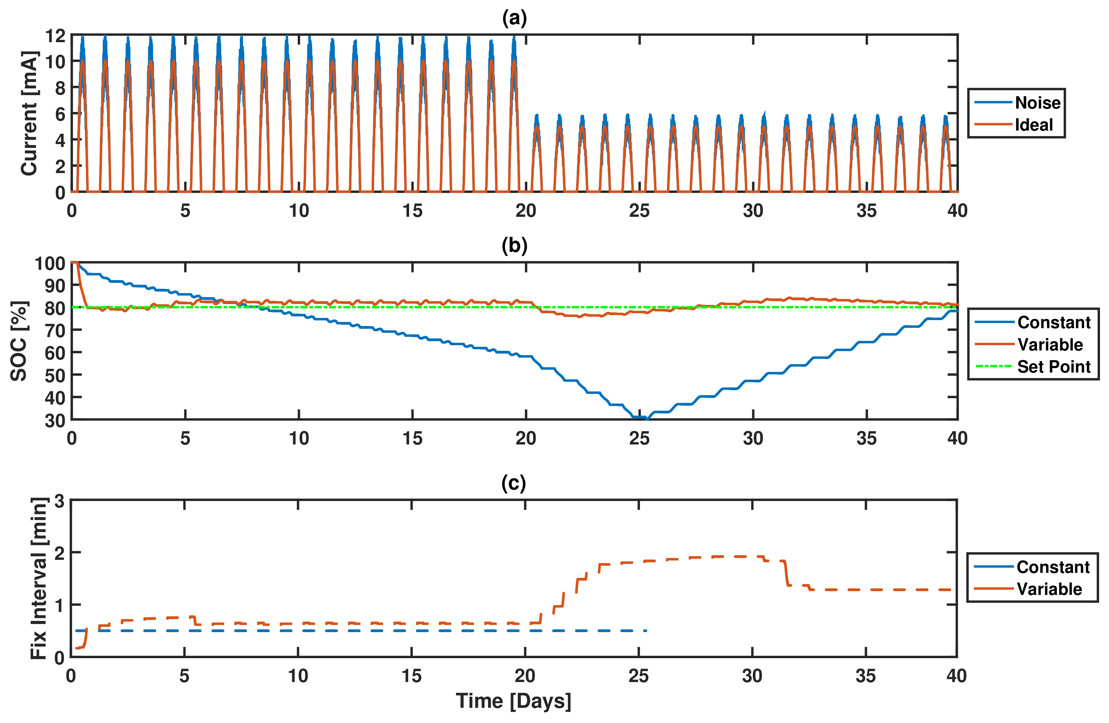
A decrease in energy available for harvesting was simulated to determine controller performance, as shown in
Figure 11. The battery and initial conditions were the same as the previous simulation setup. At first, the controller was allowed to settle at a constant fix interval before changing the PVC energy harvested, which took 6 days, plus some additional time to ensure stability and to highlight the constant fix method’s drop in SOC. The fixed collection method, in this case, was set on the aggressive side to demonstrate the battery SOC drop over a 20 days where recovery was not possible. After the PVC levels changed, on day 20, the constant fix rate model entered an unrecoverable state where data collection was stopped to attempt a battery charge that was indicated to take 20 days. The developed controller was able to make adjustments over a few days to arrive at a new fix interval that was higher than the original, 1.5 fixes per minute, and never stopped collecting data.
The opposite of diminishing energy harvesting, an increase in available energy, was also simulated, as shown in
Figure 12. The battery and initial conditions were the same as the previous simulation setup. At first, the developed controller was allowed to settle at a fix rate along with the fixed collection rate, completely draining the battery. The controller first overshot and then settled after 13 days. The PVC harvesting was kept constant for 20 days at a 5 mA peak. After 20 days, the PVC harvesting value was increased to 10 mA peak and the controller responded within a single day and then settled after 10 days. The final settled value of the increased harvesting amount was within 0.1 min of the previous simulation before the PVC peak was reduced, giving validation that the controller will settle at similar rates given similar harvesting conditions.


