Effect of Control Measures on Wheel/Rail Noise When the Vehicle Curves


Abstract
:1. Introduction
2. The Time Domain Model for Predicting Wheel/Rail Noise under Lateral Excitation
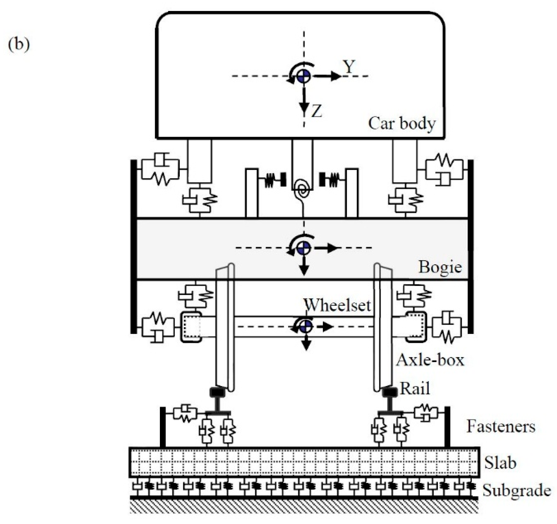
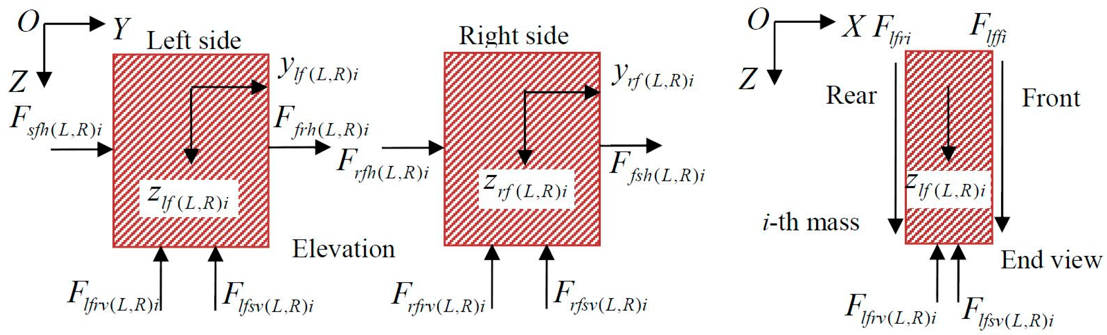
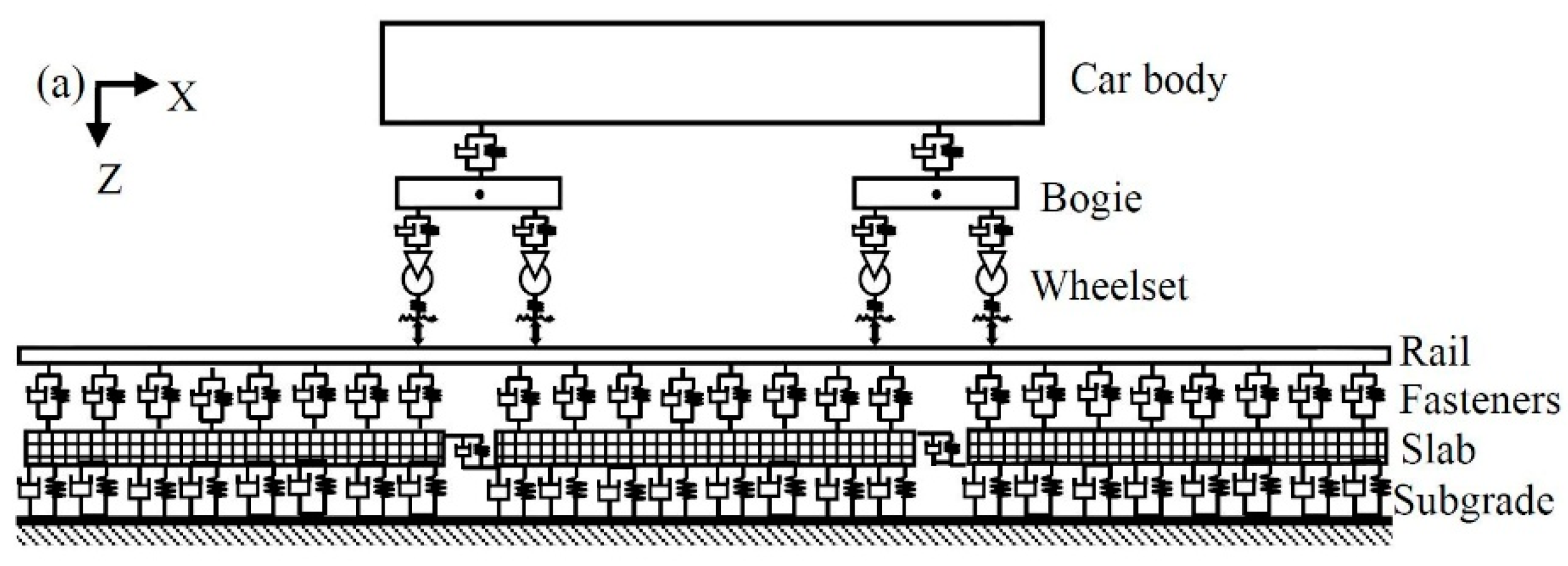
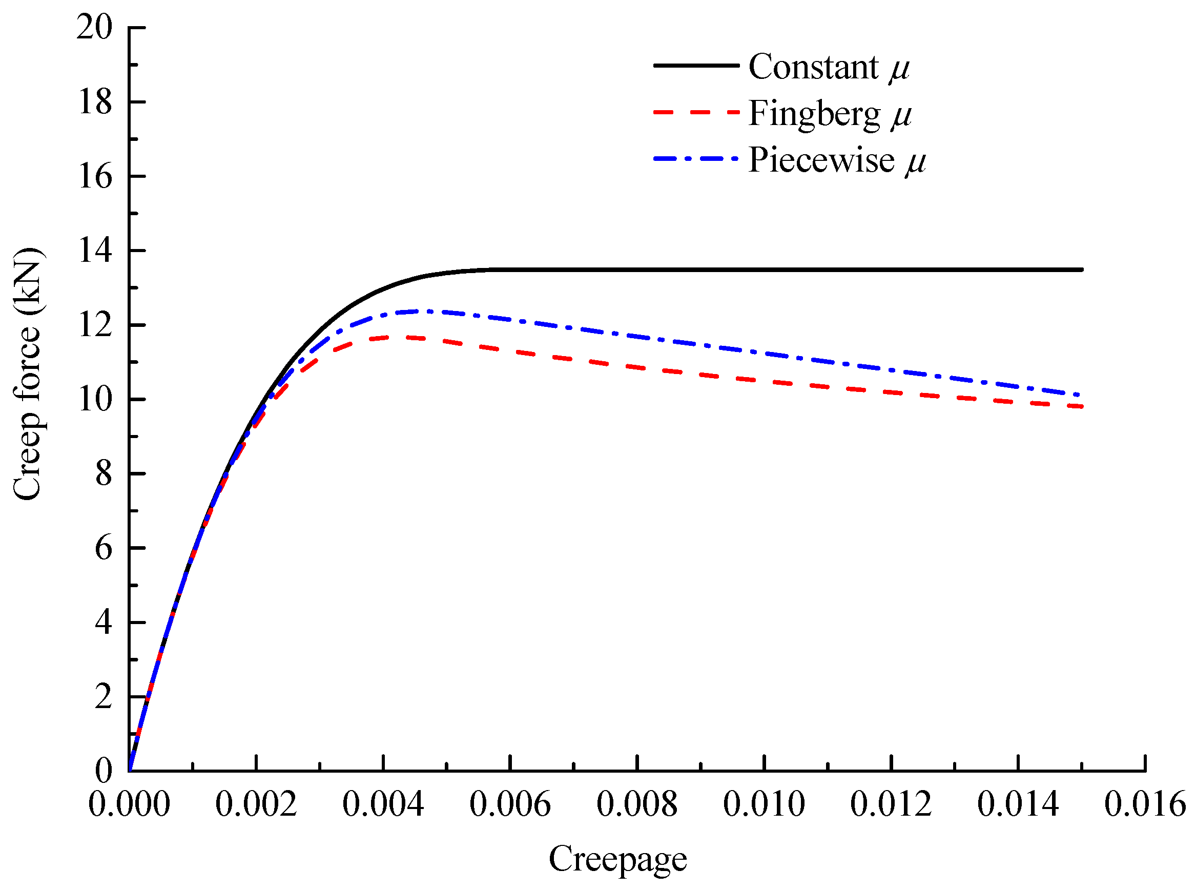
2.1. Vehicle/Track Interaction Model with Falling Friction Coefficients
2.2. The Transient Finite and Boundary Element Model for Wheel/Rail Vibration and Sound Radiation
3. Results and Discussions
3.1. Wheel/Rail Noise Prediction and Preliminary Validation
3.2. Effect of Wheel/Rail Friction Coefficients on Wheel/Rail Noise under Lateral Excitation
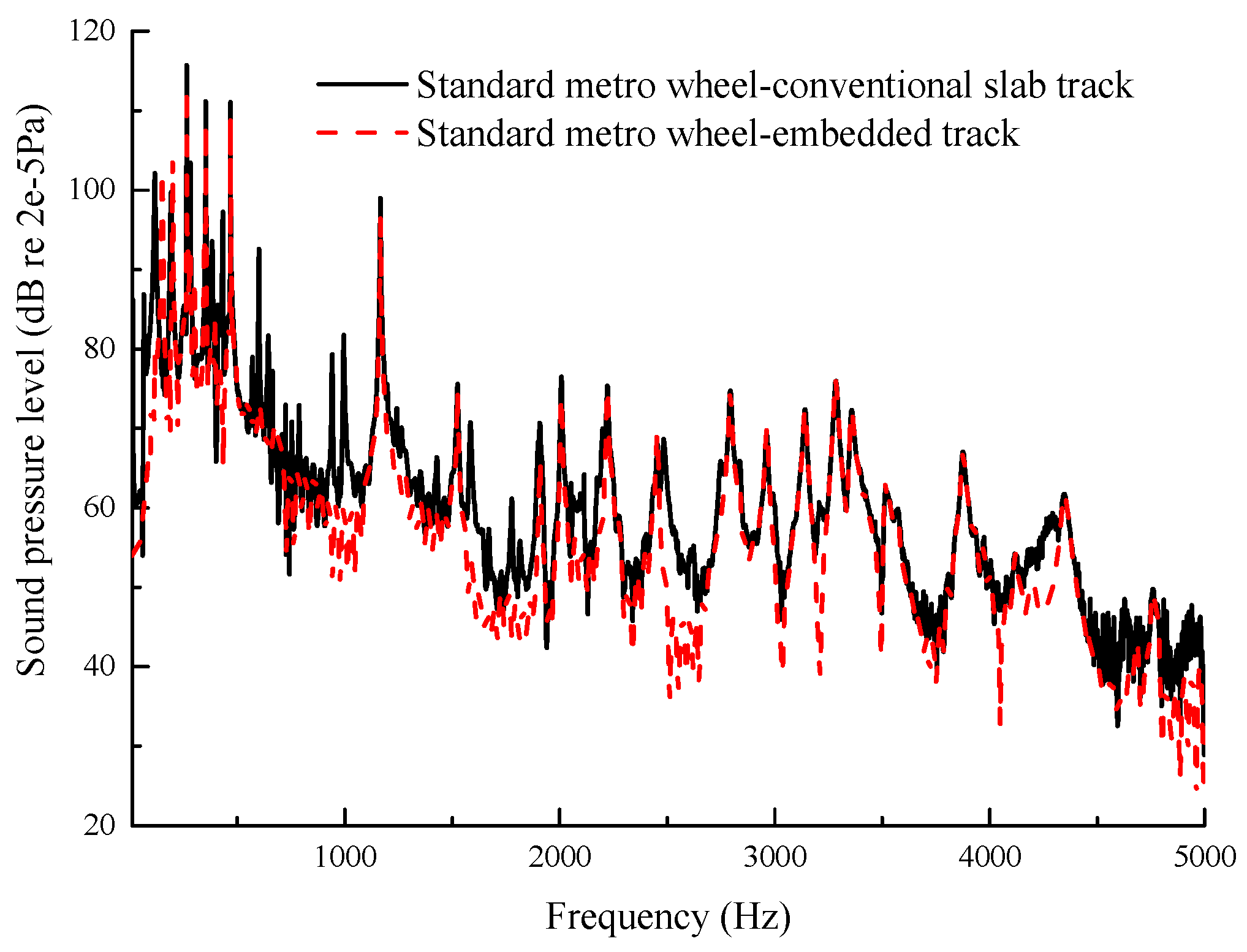
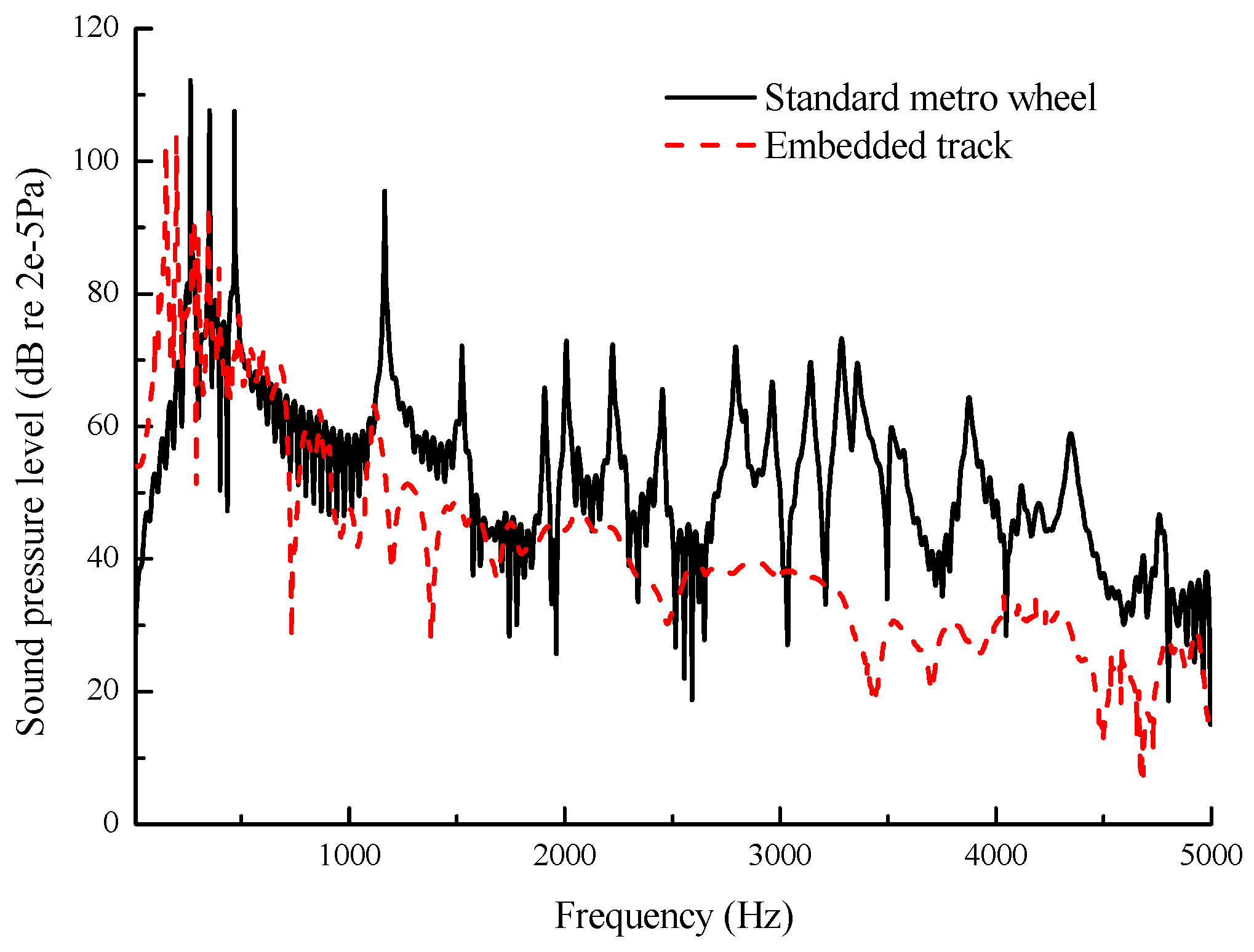
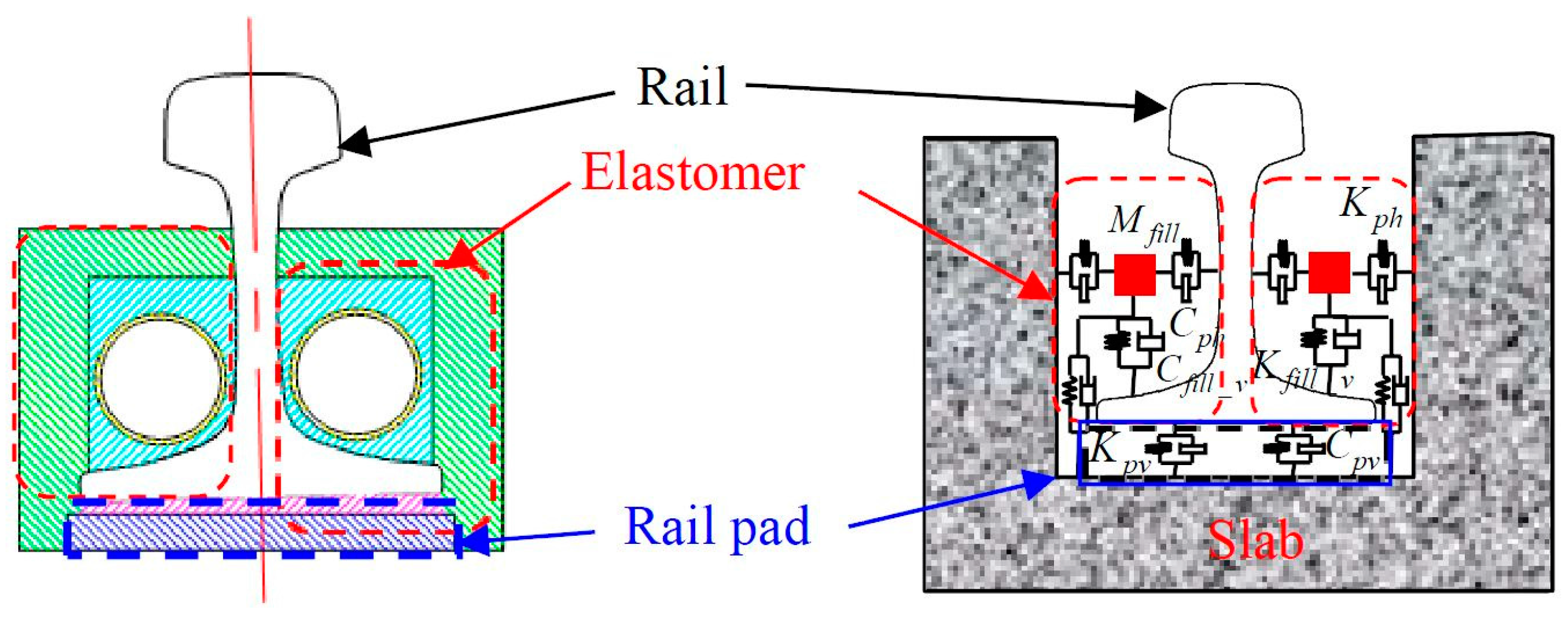
3.3. Effect of Embedded Track on Wheel/Rail Noise under Lateral Excitation
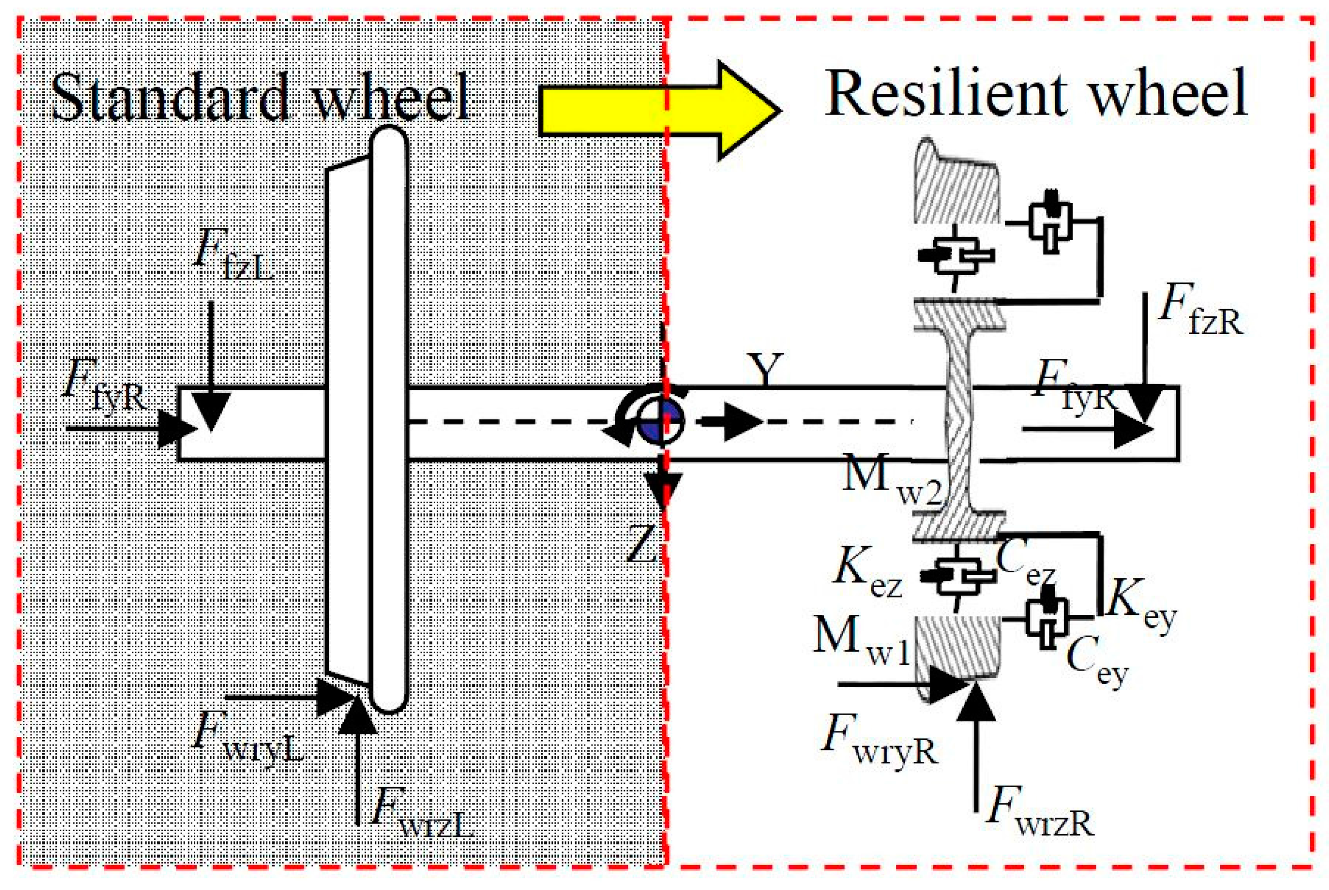
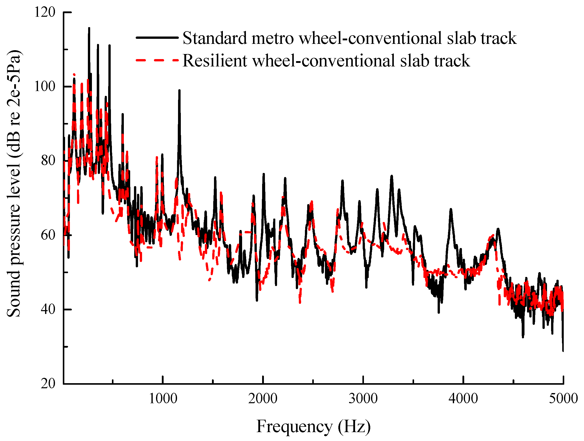
3.4. Effect of Resilient Wheel on Wheel/Rail Noise under Lateral Excitation
4. Conclusions
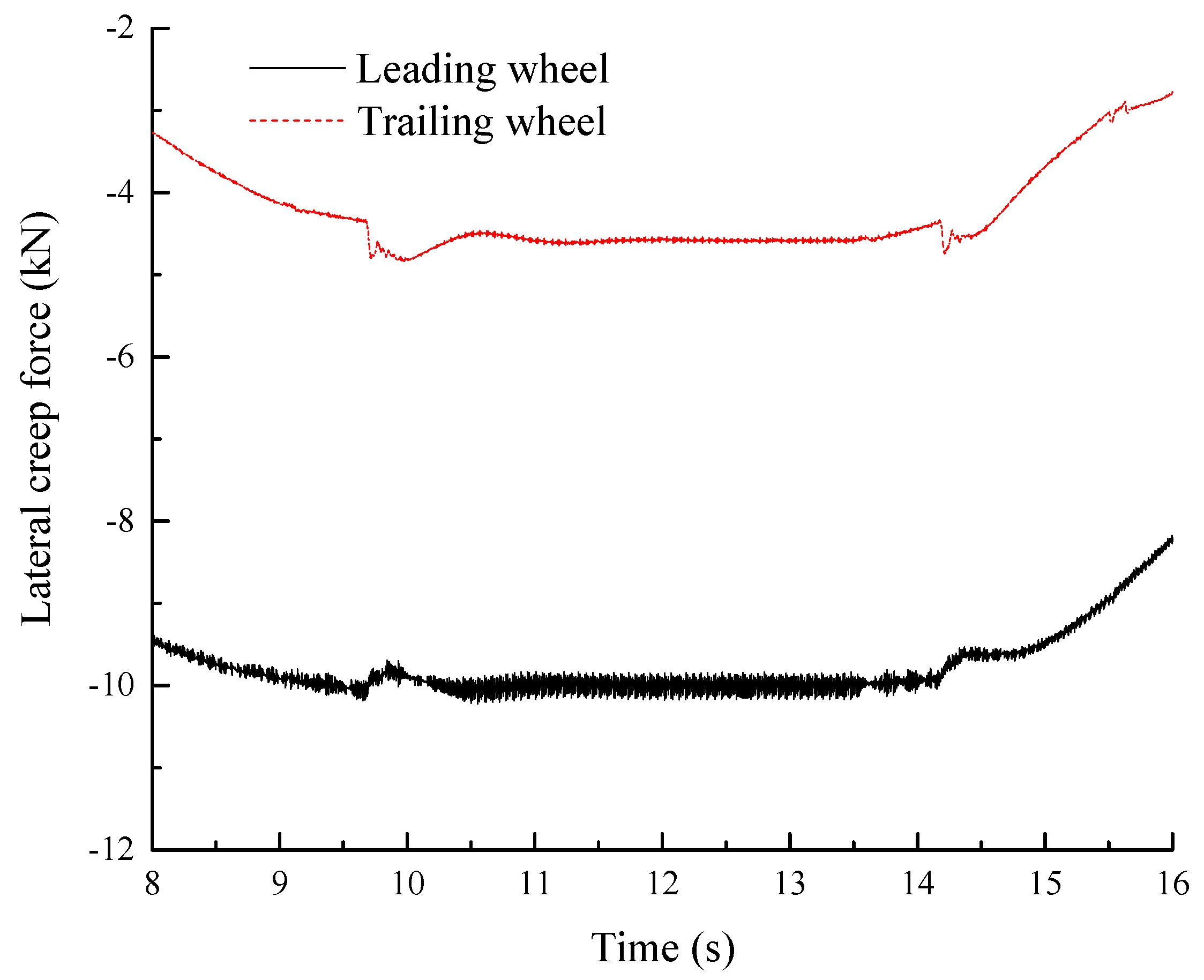
- (1)
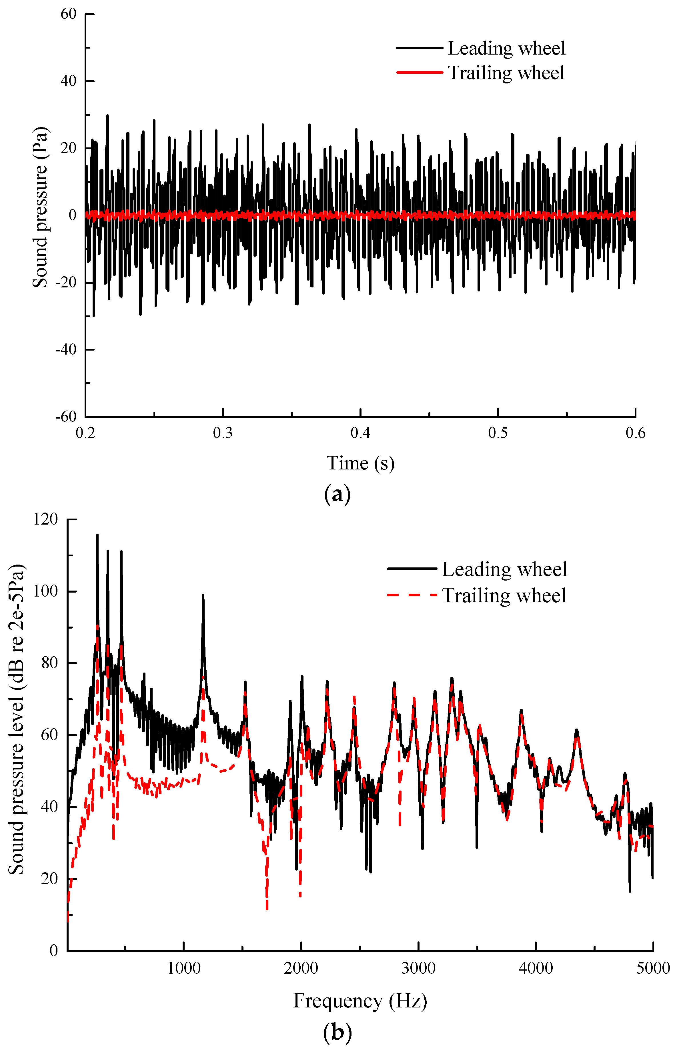
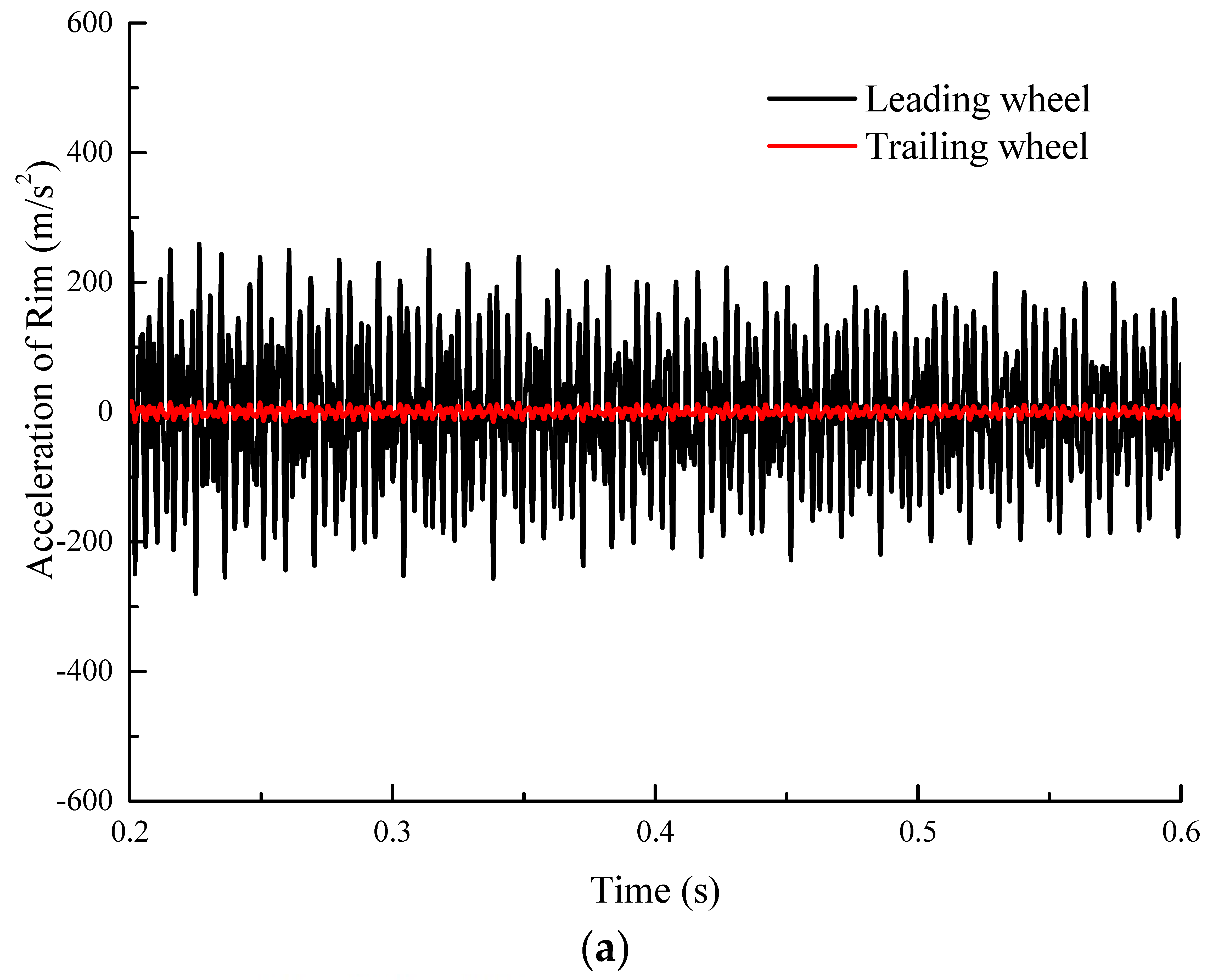
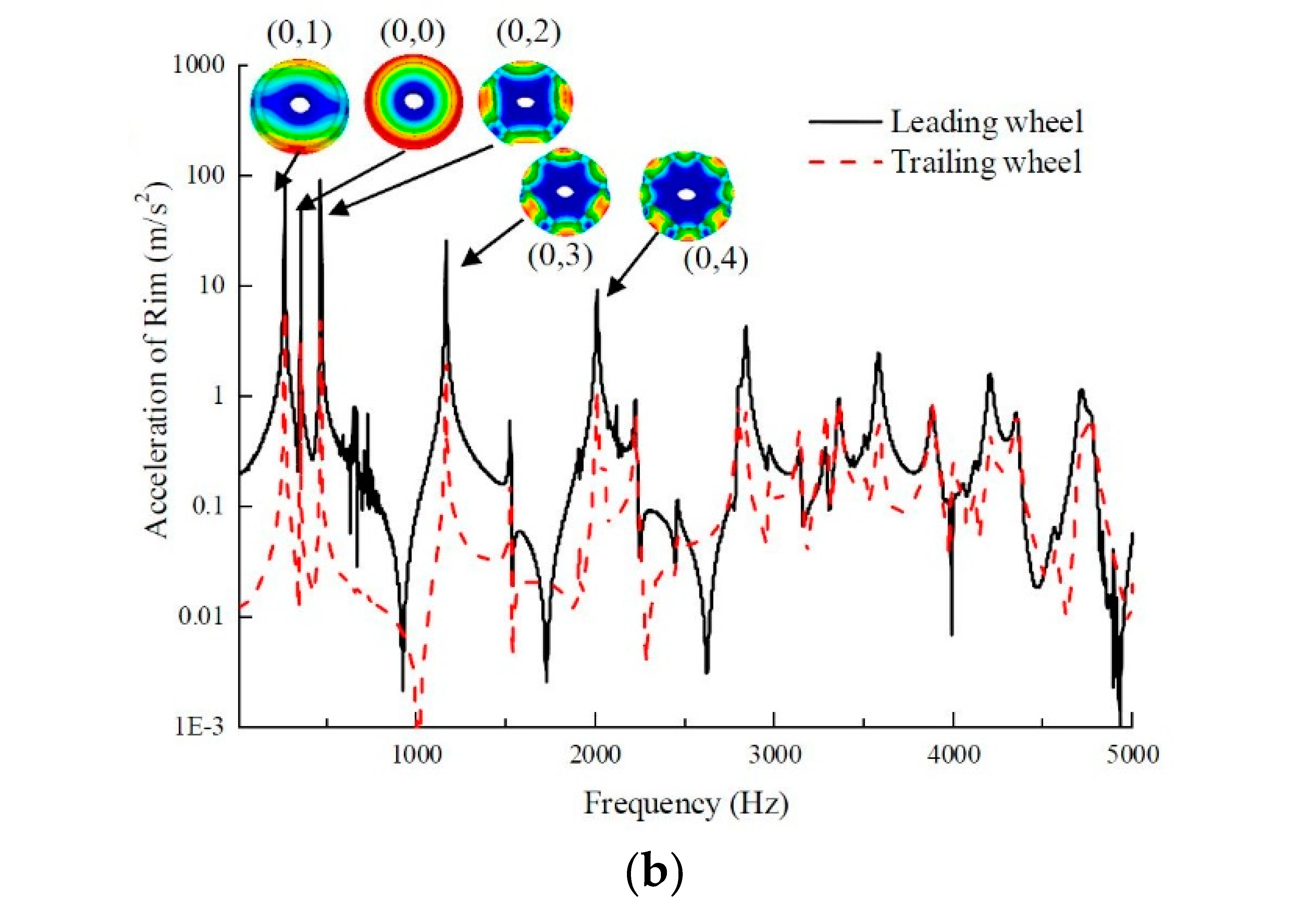
- Different wheels have different levels of wheel/rail noise when the vehicle curves. The wheel/rail noise of the leading wheel is 20 dB larger than that of the trailing wheel.
- (2)
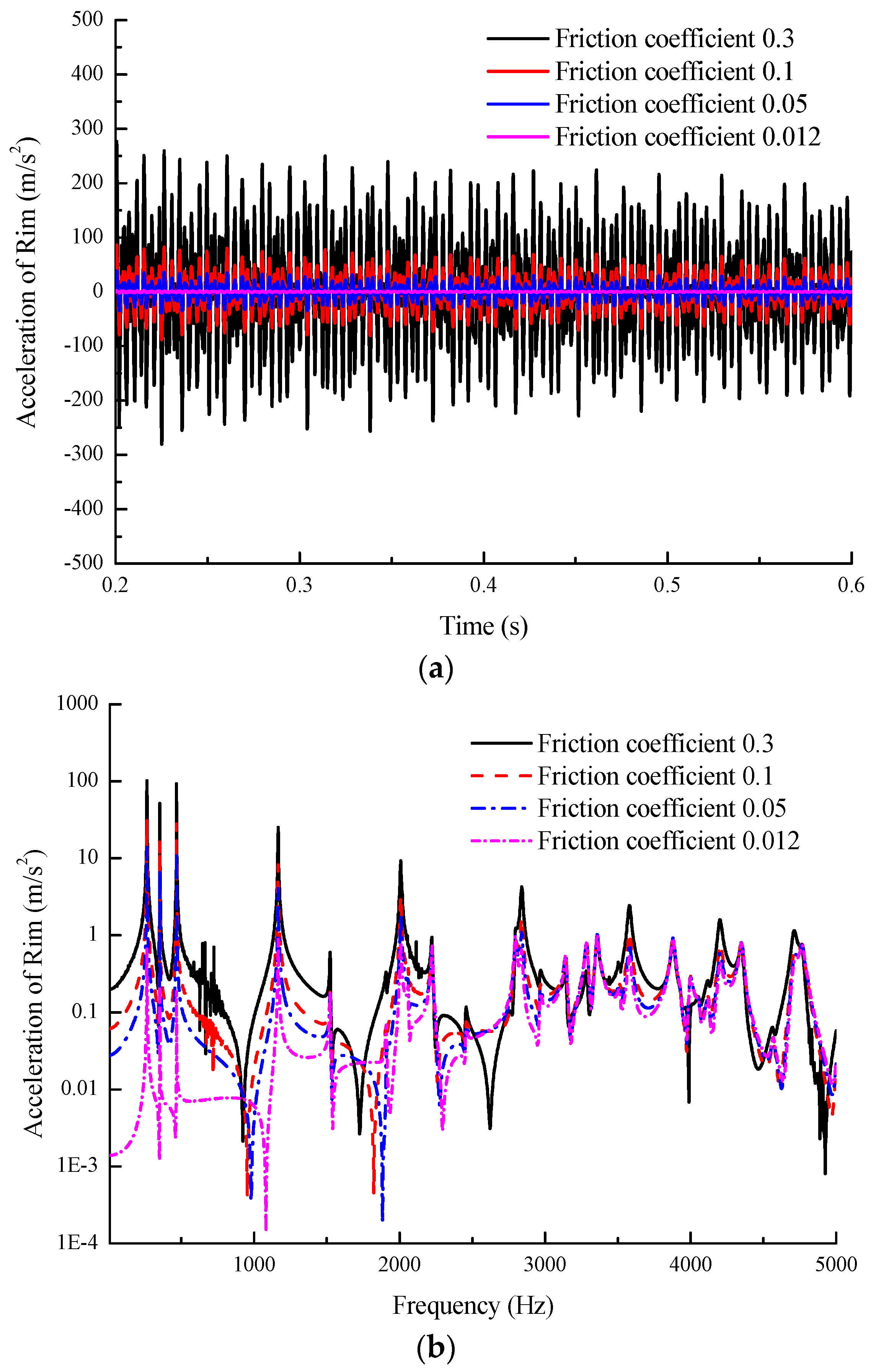
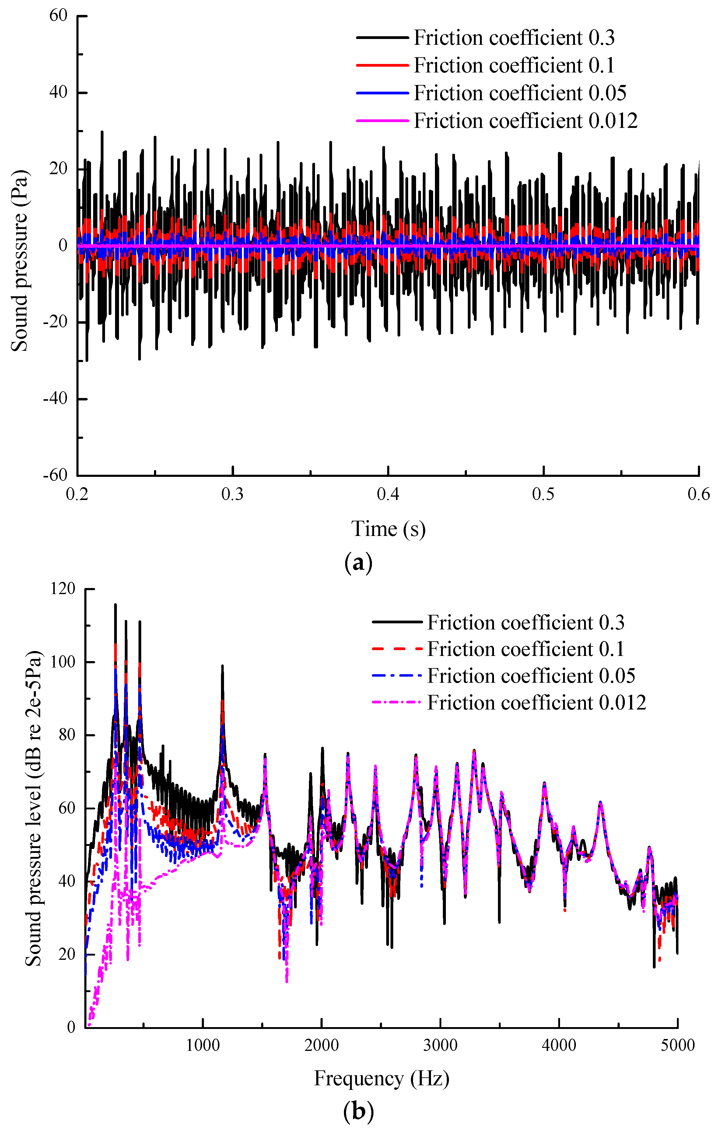
- Proper lubrication in wheel/rail interface can effectively reduce wheel/rail noise when the vehicle curves. The sound reduction of wheel considering lubricant (friction coefficient: 0.012~0.1) can reduce 10~25 dB compared to that of friction coefficient 0.3.
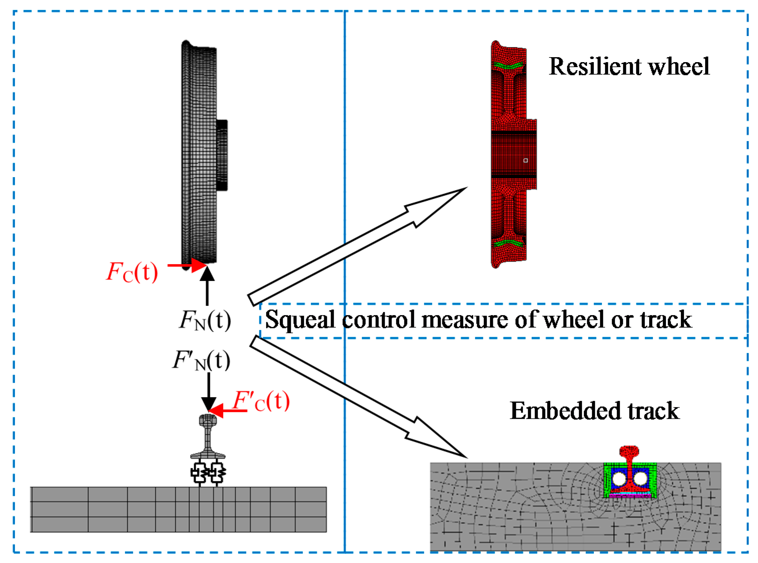
- (3)
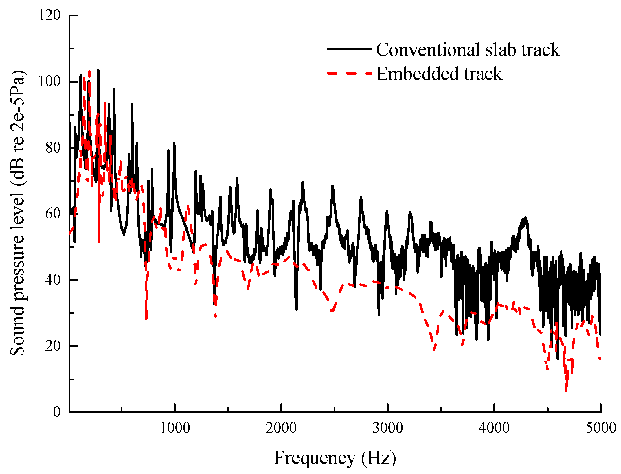
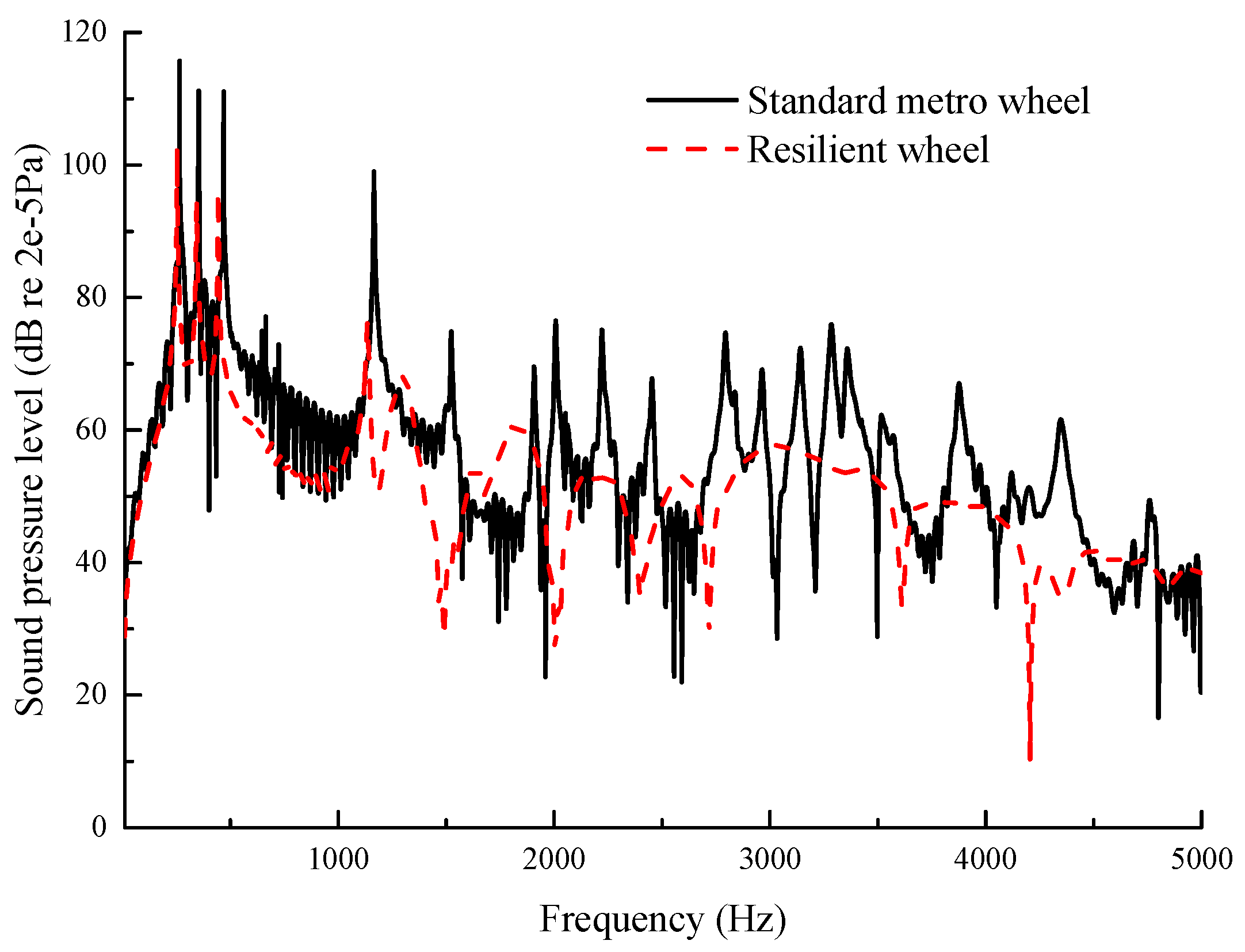
- The application of vibration and noise control measures on wheels is better than that on track when the vehicle curves. The total sound reduction of the embedded track coupled with a squealing wheel is about only 2–3 dB. However, the total sound reduction of the elastic wheel coupled with the conventional slab track is about 5–6 dB.
Acknowledgments
Author Contributions
Conflicts of Interest
References
- Rudd, M. Wheel/rail noise—Part 2: Wheel squeal. J. Sound Vib. 1976, 46, 381–394. [Google Scholar] [CrossRef]
- Thompson, D.J.; Jones, C.J.C. A review of the modelling of wheel-rail noise generation. J. Sound Vib. 2000, 231, 519–536. [Google Scholar] [CrossRef]
- Brunel, J.F.; Dufrénoy, P.; Naït, M.; Muñoza, J.L.; Demilly, F. Transient models for curve squeal noise. J. Sound Vib. 2006, 293, 758–765. [Google Scholar] [CrossRef]
- Kooijman, P.P.; Van Vliet, W.J.; Janssens, M.H.A.; de Beer, F.G. Curve squeal of railbound vehicles—Part 2: Set-up for measurement of creepage dependent friction coefficient. In Proceedings of the Internoise 2000, Nice, France, 27–30 August 2000. [Google Scholar]
- Eadie, D.T.; Santoro, M. Top-of-rail friction control for curve noise mitigation and corrugation rate reduction. J. Sound Vib. 2006, 293, 747–757. [Google Scholar] [CrossRef]
- Wetta, P.; Demilly, F. Reduction of wheel squeal noise generated on curves or during braking. In Proceedings of the 11th International Wheelset Congress, Paris, France, 18–22 June 1995. [Google Scholar]
- Brunel, J.F.; Dufrenoy, P.; Demilly, F. Modelling of squeal noise attenuation of ring damped wheels. J. Sound Vib. 2004, 65, 457–471. [Google Scholar] [CrossRef]
- Han, J.; Wen, Z.; Wang, R.; Wang, D.; Xiao, X.; Zhao, G.; Jin, X. Experimental study on vibration and sound radiation reduction of the web-mounted noise shielding and vibration damping wheel. Noise Control Eng. J. 2014, 62, 110–122. [Google Scholar] [CrossRef]
- Liu, H.; Yang, J.; Wu, T. The influences of rail vibration absorber on normal wheel-rail contact forces due to multiple wheels. J. Vib. Control 2015, 21, 275–284. [Google Scholar] [CrossRef]
- Ruiten, C.J.M. Mechanism of squeal noise generated by trams. J. Sound Vib. 1988, 120, 245–253. [Google Scholar] [CrossRef]
- Remington, P.J. Wheel/rail squeal and impact noise: What do we know? What do not we know? Where do we go from here? J. Sound Vib. 1985, 116, 339–353. [Google Scholar] [CrossRef]
- Schneider, E.; Popp, K.; Irretier, H. Noise generation in railway wheels due to rail-wheel contact forces. J. Sound Vib. 1988, 120, 227–244. [Google Scholar] [CrossRef]
- Fingberg, U. A model of wheel-rail squealing noise. J. Sound Vib. 1990, 143, 365–377. [Google Scholar] [CrossRef]
- Périard, F. Wheel-Rail Noise Generation: Curve Squealing by Trams. Ph.D. Thesis, Technische Universiteit, Delft, The Netherlands, 1998. [Google Scholar]
- Heckl, M.A.; Abrahams, I.D. Curve squeal of train wheels, part 1: Mathematical model for its generation. J. Sound Vib. 2000, 229, 669–693. [Google Scholar] [CrossRef]
- Beer, F.G.; Janssens, M.H.A.; Kooijman, P.P. Squeal noise of rail-bound vehicles influenced by lateral contact position. J. Sound Vib. 2003, 267, 497–507. [Google Scholar] [CrossRef]
- Monk-Steel, A.D.; Thompson, D.J. Models for railway curve squeal noise. In Proceedings of the 8th Conference on Recent Advances in Structural Dynamics, Southampton, UK, 14–16 July 2003. [Google Scholar]
- Chiello, O.; Ayasse, J.B.; Vincent, N.; Koch, J.R. Curve squeal of urban rolling stock- Part 3: Theoretical model. J. Sound Vib. 2006, 293, 710–727. [Google Scholar] [CrossRef]
- Cataldi-Spinola, E.; Glocker, C. Curve squealing of railroad vehicles. In Proceedings of the ENOC-2005, Eindhoven, The Netherlands, 7–12 August 2005. [Google Scholar]
- Kalker, J.J. Survey of wheel-rail rolling contact theory. Veh. Syst. Dyn. 1979, 5, 317–358. [Google Scholar] [CrossRef]
- Xie, G.; Allen, P.D.; Iwnicki, S.D.; Alonso, A.; Thompson, D.J.; Jones, C.J.; Huang, Z.Y. Introduction of falling friction coefficients into curving calculations for studying curve squeal noise. Veh. Syst. Dyn. 2006, 44 (Suppl. 1), S261–S271. [Google Scholar] [CrossRef]
- Thompson, D.J.; Janssens, M.H.A. Theoretical Manual, Version 2.4; TNO Report, No. TPD-HAG-RPT-930214 (Revised); TNO: Hague, The Netherlands, 1997. [Google Scholar]
- Huang, Z. Theoretical Modelling of Railway Curve Squeal. Ph.D. Thesis, University of Southampton, Southampton, UK, 2007. [Google Scholar]
- Hoffmann, N.; Fischer, M.; Allgaier, R.; Gaul, L. A minimal model for studying properties of the mode-coupling type instability in friction induced oscillations. Mech. Res. Commun. 2002, 29, 197–205. [Google Scholar] [CrossRef]
- Hoffmann, N.; Gaul, L. Effects of damping on mode-coupling instability in friction induced oscillations. J. Appl. Math. Mech. 2003, 83, 524–534. [Google Scholar] [CrossRef]
- Sinou, J.J.; Jezequel, L. Mode coupling instability in friction-induced vibrations and its dependency on system parameters including damping. Eur. J. Mech.-A/Solids 2007, 26, 106–122. [Google Scholar] [CrossRef]
- Thompson, D.J.; Squicciarini, G.; Ding, B. A state-of-the-art review of curve squeal noise: Phenomena, mechanisms, modelling and mitigation. In Proceedings of the 12th International Workshop on Railway Noise, Terrigal, Australia, 12–16 September 2016. [Google Scholar]
- Jin, X.S.; Wen, Z.F. Effect of discrete track support by sleepers on rail corrugation at a curved track. J. Sound Vib. 2007, 315, 279–300. [Google Scholar] [CrossRef]
- Xiao, X.B.; Jin, X.S.; Wen, Z.F. Effect of disabled fastening systems and ballast on vehicle derailment. J. Vib. Acoust. 2007, 129, 217–229. [Google Scholar] [CrossRef]
- Han, J.; Zhao, G.T.; Xiao, X.B.; Wen, Z.F.; Guan, Q.H.; Jin, X.S. Effect of softening of cement asphalt mortar on vehicle operation safety and track dynamics. J. Zhejiang Univ. SCIENCE A 2015, 16, 976–986. [Google Scholar] [CrossRef]
- Han, J.; Zhao, G.T.; Sheng, X.Z.; Jin, X.S. Study on the subgrade deformation under high-speed train loading and water-soil interaction. Acta Mech. Sin. 2016, 32, 233–243. [Google Scholar] [CrossRef]
- Ling, L.; Dhanasekar, M.; Thambiratnam, D.P.; Sun, Y.Q. Lateral impact derailment mechanisms, simulation and analysis. Int. J. Impact Eng. 2016, 94, 36–49. [Google Scholar] [CrossRef]
- Ling, L.; Dhanasekar, M.; Thambiratnam, D.P.; Sun, Y.Q. Minimising lateral impact derailment potential at level crossings through guard rails. Int. J. Mech. Sci. 2016, 113, 49–60. [Google Scholar] [CrossRef]
- Zhai, W.M. Two simple fast integration methods for large-scale dynamic problems in engineering. Int. J. Numer. Methods Eng. 1996, 39, 4199–4214. [Google Scholar] [CrossRef]
- Shen, Z.Y.; Hedrick, J.K.; Elkins, J.A. A comparison of alternative creep-force models for rail vehicle dynamic analysis. Veh. Syst. Dyn. 1983, 12, 79–83. [Google Scholar] [CrossRef]
- Wu, T.W. Boundary Element Acoustics; WIT Press: Southampton, UK, 2005. [Google Scholar]
- Ling, L.; Han, J.; Xiao, X.; Jin, X. Dynamic behavior of an embedded rail track coupled with a tram vehicle. J. Vib. Control 2017, 23, 2355–2372. [Google Scholar] [CrossRef]
- Zhao, Y.; Li, X.; Lv, Q.; Jiao, H.; Xiao, X.; Jin, X. Measuring, modelling and optimising an embedded rail track. Appl. Acoust. 2017, 116, 70–81. [Google Scholar] [CrossRef]


| Notations | Parameters | Values (End) |
|---|---|---|
| M/I | Body inertia | |
| Mc | Car body mass (kg) | 2.16 × 10⁴ |
| Mb | Bogie mass (kg) | 4.00 × 10³ |
| Mw | Wheelset mass (kg) | 1.86 × 10³ |
| Icx | Car body roll moment of inertia (kg·m2) | 3.11 × 10⁴ |
| Icy | Car body pitch moment of inertia (kg·m2) | 8.61 × 10⁵ |
| Icz | Car body yaw moment of inertia (kg·m2) | 8.56 × 10⁵ |
| Ibx | Bogie roll moment of inertia (kg·m2) | 1.19 × 10³ |
| Iby | Bogie pitch moment of inertia (kg·m2) | 8.76 × 10² |
| Ibz | Bogie yaw moment of inertia (kg·m2) | 2.10 × 10³ |
| Iwx | Wheelset roll moment of inertia (kg·m2) | 1.04 × 10³ |
| Iwy | Wheelset pitch moment of inertia (kg·m2) | 1.37 × 10² |
| Iwz | Wheelset yaw moment of inertia (kg·m2) | 1.04 × 10³ |
| K/C | Primary suspension | |
| Kpx | Longitudinal stiffness (MN/m) | 17.62 |
| Kpy | Lateral stiffness (MN/m) | 9.62 |
| Kpz | Vertical stiffness (MN/m) | 0.60 |
| Cpz | Vertical damping coefficient (kN·s/m) | 13.00 |
| K/C | Secondary suspension | |
| Ksx | Longitudinal stiffness (MN/m) | 0.16 |
| Ksy | Lateral stiffness (MN/m) | 0.16 |
| Ksz | Vertical stiffness (MN/m) | 1.39 |
| Csy | Lateral damping coefficient (kN·s/m) | 23.00 |
| Csz | Vertical damping coefficient (kN·s/m) | 25.00 |
| L/D/H | Dimension | |
| Rw | Wheel radius (m) | 0.42 |
| Lv | Vehicle length (m) | 19.5 |
| Lb | Distance between two axles of a bogie (m) | 2.3 |
| Lc | Distance between two bogie centers (m) | 12.6 |
| Dps | Lateral span of primary suspensions (m) | 2.01 |
| Dss | Lateral span of secondary suspensions (m) | 1.9 |
| Hbw | Height of bogie centre from wheelset centre (m) | 0.069 |
| Hcb | Height of car body centre from bogie centre (m) | 1.37 |
© 2017 by the authors. Licensee MDPI, Basel, Switzerland. This article is an open access article distributed under the terms and conditions of the Creative Commons Attribution (CC BY) license (http://creativecommons.org/licenses/by/4.0/).
Share and Cite
Han, J.; He, Y.; Xiao, X.; Sheng, X.; Zhao, G.; Jin, X. Effect of Control Measures on Wheel/Rail Noise When the Vehicle Curves. Appl. Sci. 2017, 7, 1144. https://doi.org/10.3390/app7111144
Han J, He Y, Xiao X, Sheng X, Zhao G, Jin X. Effect of Control Measures on Wheel/Rail Noise When the Vehicle Curves. Applied Sciences. 2017; 7(11):1144. https://doi.org/10.3390/app7111144
Chicago/Turabian StyleHan, Jian, Yuanpeng He, Xinbiao Xiao, Xiaozhen Sheng, Guotang Zhao, and Xuesong Jin. 2017. "Effect of Control Measures on Wheel/Rail Noise When the Vehicle Curves" Applied Sciences 7, no. 11: 1144. https://doi.org/10.3390/app7111144
APA StyleHan, J., He, Y., Xiao, X., Sheng, X., Zhao, G., & Jin, X. (2017). Effect of Control Measures on Wheel/Rail Noise When the Vehicle Curves. Applied Sciences, 7(11), 1144. https://doi.org/10.3390/app7111144