1. Introduction
It was a breakthrough discovery that the irregular motion, with a broadband frequency spectrum with Gaussian-like distribution and extreme sensitivity to changes of the initial conditions, can be observed in the class of autonomous dynamical systems with three degrees of freedom. Such behavior, now known as chaotic solution, has often been misinterpreted as a mixture of harmonic signals and noise. Research works have focused on nonlinear dynamics connected with chaos theory, proving that chaos is not a numerical artifact, but represents robust behavior and has nothing to do with stochastic processes.
Since 1963, when Lorenz first noticed and described deterministic chaos [
1], numerical and experimental observations of the chaotic attractors have been reported in many scientific fields. Chaotic phenomena have been observed in reaction–diffusion systems in chemistry [
2], fundamental models of classical mechanics such as pendulum with periodic excitations [
3], mathematical models describing fluid dynamics [
4] and hydrodynamics [
5]. Unique features of chaotic signals have been registered in brain activity [
6] or electrocardiogram [
7] data. The emergence of a population of different species in biology [
8], commodity exchange in economy [
9] and time-dependent models of many ecological situations [
10] are other examples of dynamical systems that are subject to chaotic dynamics. By referring to this knowledge, the presence of chaos in an evolution equation [
11] and electronic circuits (both lumped and with spread parameters) seems to be obvious and logical.
Besides the mentioned research, works narrowly targeting specific scientific areas, general analysis of differential equations and properties of available solutions, automatically touches on multiple branches of physics. Intensive studies on chaotic phenomena in the last five decades reveal that this kind of complex behavior is much less rare than was initially expected. Pioneering works [
12,
13], which searched for algebraically simple chaotic flows, present a number of third-order autonomous mathematical models with only six terms, including scalar nonlinearity and the associated chaotic behavior. After the publication of these works, searching for mathematical models that exhibit chaotic motion became a favorite topic of research studies. Of course, the rusticity of describing a set of ordinary differential equations leads to a simple lumped circuit, which is capable of modelling such dynamics with two active and seven passive elements, as shown in [
14]. However, canonical realizations of chaotic oscillators (in the sense of minimum component count) usually have model parameters expressed as functions (generally nonlinear) of the circuit parameters. Typical examples of very simple chaotic flows can be expressed by a single third-order differential equation as previously addressed [
15]. Such systems have a direct relation with Newtonian motion dynamics, since individual state variables can be interpreted as position, velocity and acceleration. The implementation of a single higher-order differential equation as an electronic circuit is very simple: the cascade of two-port integrators is put together with multiple feedback branches.
A primary assumption, which has only recently been disproven, is that a combination of several saddle-focus [
16,
17] equilibrium points is required for the emergence of dense in state space chaotic attractors with a fractal geometric dimension. However, it turns out that saddle-node [
18] types of equilibria, with the same stability index as saddle focusses, can also be responsible for the evolution of the chaotic attractor. Finally, after years of research dedicated to the autonomous dynamical systems, it seems that the existence of the multiple fixed points is not necessary for a vector field to exhibit chaotic behavior. Strange attractors can also be observed in dynamical systems with a single unstable node equilibrium, as previously demonstrated [
19]. The most surprisingly unstable fixed points, which are normally responsible for strange attractor excitation and extreme sensitivity of dynamical system behavior to the initial conditions, can be changed into a single stable fixed point [
20,
21] or a pair of stable equilibria [
22]. Chaos can be observed in isolated dynamical systems with fixed points degenerating into plane geometrical structures such as a line [
23], circle [
24], rounded square and square [
25]. The mathematical system discovered by the authors can be considered as a member of this group. The placement and shape of the strange attractor, with respect to equilibrium structure, suggests that only a fragment of a line, circle or square is active in the evolution of chaos. Interesting mathematical models with curve of equilibria are briefly discussed in the summarizing publication [
26] and simple sets of the ordinary differential equations with equilibria degenerated into surfaces are a topic of paper [
27]. Exhaustive research in this area reveals several third-order chaotic dynamical systems without singular or degenerated equilibria; for details, consult [
28] or [
29].
Since the investigated mathematical model in the upcoming section has a dimensionless state, variables as well as internal system parameters can have different physical meanings. This is how chaos theory connects different scientific disciplines; through the universality and auxiliary time scales.
2. Mathematical Methods, Discovered Model and Numerical Analysis
The very nature of chaos excludes the existence of closed-form analytic solution, as chaotic waveform is no long-term predictable. However, there are methods that separate regular behavior from irregular, using noise-like dynamic motion. The basic principle behind these methods is the numerical integration of differential equations. The knowledge of describing mathematical models allows the use of a trustworthy motion quantifier; the largest Lyapunov exponent (LE). This real number is positive in the case of the exponential divergence of two neighboring state trajectories, that is, the positive value of LE indicates chaos, while zero denotes periodic or quasi-periodic behavior and the negative value stands for a fixed point trivial solution. It should be mentioned that LE can also be extracted from a data sequence. However, this process and its superior procedure known as state attractor reconstruction is less precise, returns incorrect results in the case of wrong choices of method input parameters and should be chosen if the mathematical model is unknown, that is, the dynamical system is in the form of a black box.
2.1. Chaos Localization and Search Algorithm
Application of the LE concept in the chaos localization procedure can be automatized and has three consequent steps. The first step is the specification of the mathematical model, that is, the set of ordinary differential equations should be explicitly defined. This is a place where additional requirements for dynamical flow can be pronounced, such as the existence of hyperbolic equilibrium and its location in state space. The second step is defining the degree of freedom for upcoming tabularized calculations. These n parameters must be chosen carefully and should be able to fold the vector field in a different fashion or change the nature of dynamical flow without changing or moving the predefined equilibrium. This means that parameters leading to the unwanted properties of a dynamical system will be excluded from the calculated grid. If such exclusion is not possible, penalization of objective function can do the trick as well. The third step is the repeated calculation of LE in n-dimensional hyperspace of the chosen free internal system parameters. To reduce time demands, number n should be kept small. Due to inevitable numerical errors in the LE calculation, sets of parameters leading to the positive largest LE are stored and verified by sequential hand-made numerical verification and visual confirmation of the attractor.
Values of LE are an independent norm used in the process of calculation, such that the standard distance in Euclidean space has been adopted (supplemented by Gram–Smith orthogonalization). Since the analyzed vector field is polynomial, there are no problems with the discontinuity of gradients. Active calculation of LE begins if the state under inspection is part of the attractor, that is, the transient motion is omitted. Achieved values of LE in each step of the search procedure (using final iteration time 104) were verified by considering different initial conditions randomly picked in the vicinity of the state space origin, where trajectory is strongly pushed towards chaotic attractor. The value of the largest LE was adopted if it showed closely related values and insensitivity.
Note that the approach described above represents a time-consuming brute force numerical method and is only allowed thanks to the availability of the computational power of contemporary personal computers and workstations. Since individual calculations of LE for the different set of free parameters are totally independent, the hyperspace of model parameters can be arbitrarily divided into smaller pieces and distributed over multiple computational cores. Thus, parallel processing applied on a chaos location algorithm is logical and represents a huge advantage here. Routine, as discussed above and shown by the results achieved in this work, has been reached by using Matlab and the build-in toolbox of Compute Unified Device Architecture (CUDA) technology, invented and distributed by NVIDIA company.
2.2. New Mathematical Model of Chaotic Dynamical System
By considering motivation and the numerical approach described above, the following set of three dimensionless differential equations has been discovered and positively tested for chaotic solution:
where
a = 12
b = 0.4 are internal system parameters and
r = 1 represents the offset of hyperbolic equilibrium structure. The last equation directly defines the equilibrium object located on plane
z = 0. Both parameters
a and
b can be used to observe different route to chaos scenarios and evolution of a typical strange attractor, while parameter
r can be a fixed value. Dynamical system (1) is dissipative and volume element
V0 is contracted by the flow into
V0·exp(−
a·
z). That is, the rate of contraction is a function of state variable
z. Flow linearization given by the Jacobi matrix defined around equilibrium structure equals
Due to this expression of Jacobi matrix, a corresponding characteristic equation is also the function of point on the hyperbolic-shaped equilibrium structure, namely
Considering equilibrium plane and using curve parametrization, we can get the following simplified characteristic polynomial along with associated eigenvalues:
Thus, one eigenvalue is always zero and the remaining two eigenvalues form a complex conjugated pure imaginary pair if y > 1/√(2a) and two real eigenvalues with opposite signs otherwise. Dynamical flow near the equilibrium structure forms the most unexpected type of local geometry: center. Choice of the initial conditions close to equilibrium leads to the periodic oscillations. There is a coexistence of three (at least, as other attracting sets are not impossible but remain a mystery) types of solution: limit cycle, chaos and unbounded. Dynamical motion is invariant under the coordinate change y ↔ −y and z ↔ −z.
2.3. Numerical Analysis of Ordinary Differential Equations
A numerical integration of a dynamical system (1) with initial conditions
x0 = (0 0 0)
T, final time
tmax = 2000 s and time step Δ
t = 0.01 s by using Mathcad and the built-in fourth-order Runge–Kutta method is shown in
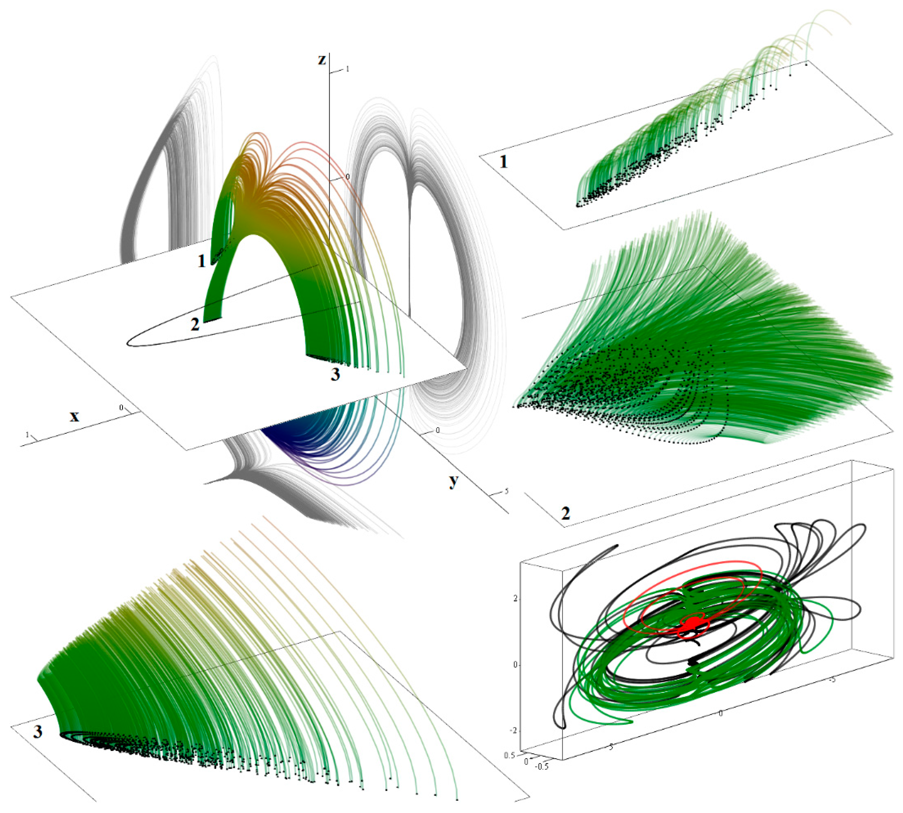
Figure 1. The same method with final time
tmax ∈ (1, 10) is used to illustrate the local dynamical behavior near equilibrium, as demonstrated by means of
Figure 2. Periodic solutions provided in this figure are excited by choosing the following sets of the initial conditions:
x0 = (−0.8 ± 0.1 0)
T,
x0 = (−0.8 ± 0.5 0)
T,
x0 = (−0.8 ± 0.8 0)
T,
x0 = (−0.2 ± 0.1 0)
T,
x0 = (−0.2 ± 0.5 0)
T and
x0 = (−0.2 ± 0.8 0)
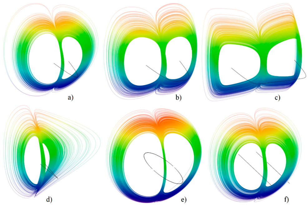
T. Numerical experiments show that the equilibrium structure can be seriously deformed while chaotic motion is still preserved. In fact, only a portion of hyperbolic function is responsible for the formation of the typical strange attractor as evident from the numerically integrated chaotic attractors provided in
Figure 3. Of course, considering piecewise linear approximation of hyperbolic function does not ease the analysis of global behavior of the investigated dynamical system. Note, the degradation of the hyperbolic function into two parallel line segments leads to the characteristic in Equation (3) with the last term missing. This means that the local behavior of dynamical flow near the equilibrium plane
z = 0 remains the same. However, deformation of equilibria into circle changes simplified the characteristic polynomial into
where
r is a circle radius and numerical values of eigenvalues depend on the state variable
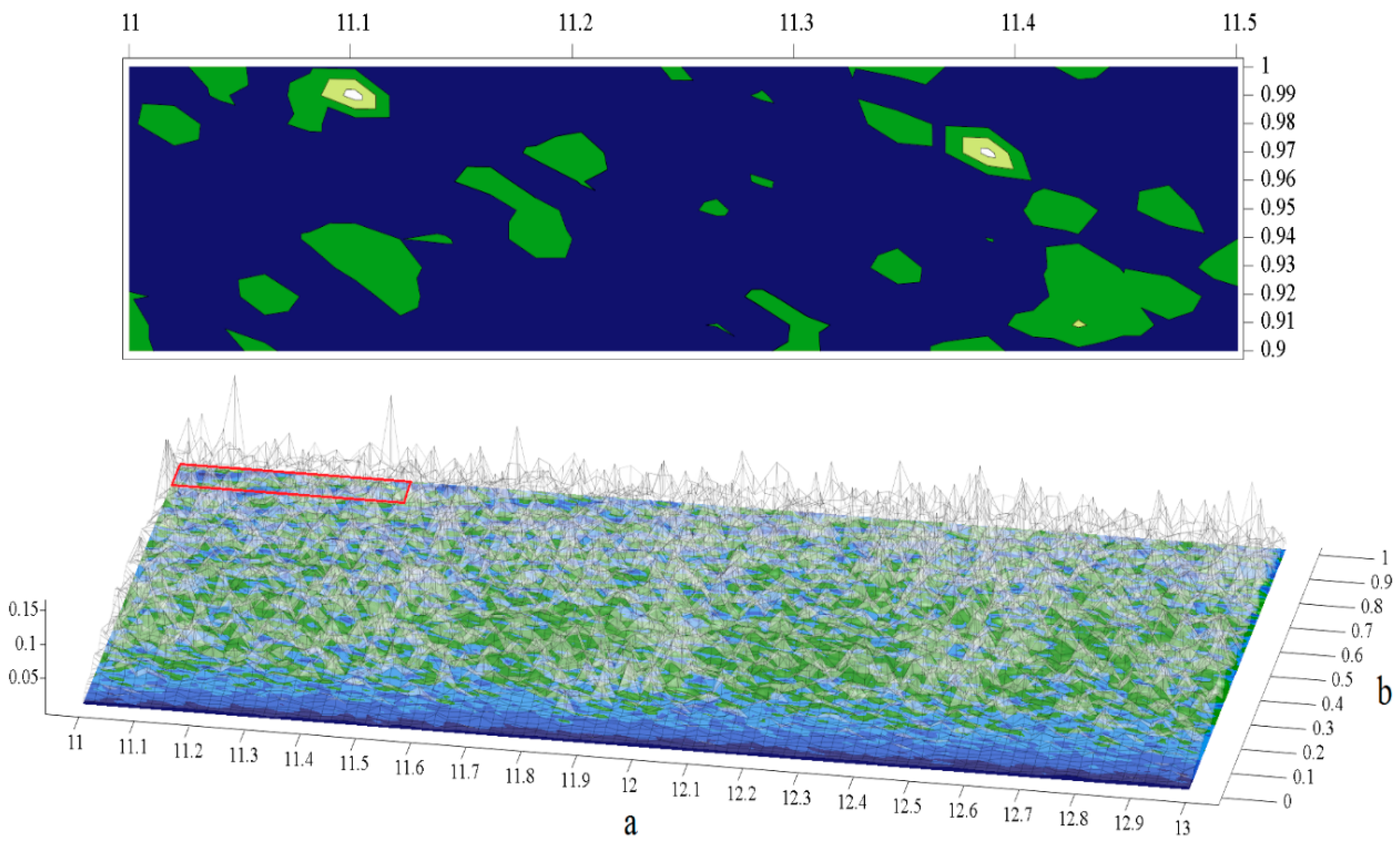
x. The regions of chaos can be visualized by plotting the largest LE as a function of the internal system parameters. The high-resolution graph having 201 × 101 (step for both parameters is 0.01) points is plotted in
Figure 4. Note that these regions are quite wide and surrounded by an unbounded solution, which means that the chaotic attractor at this moment seems to be experimentally observable.
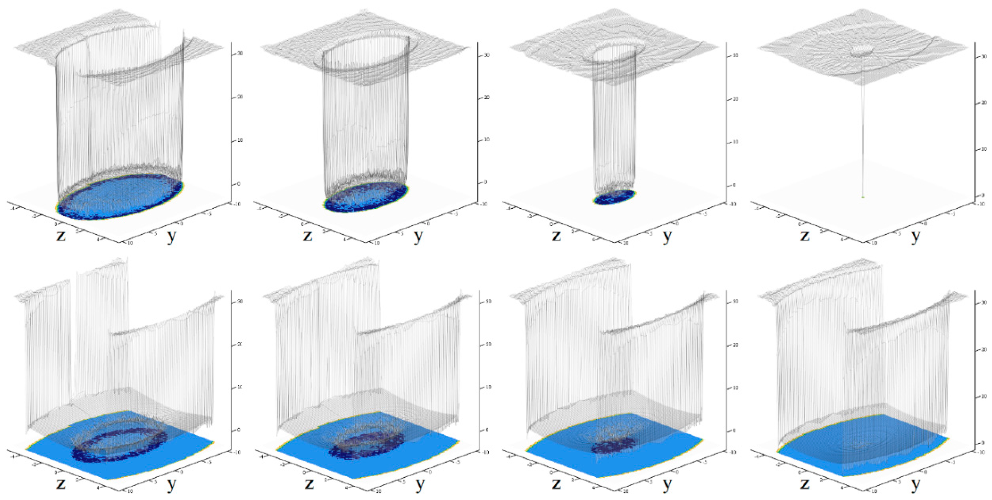
From the viewpoint of practical realization and potential applications, the basins of attraction for a chaotic attractor should be specified. So far, we admit existence of the attracting limit sets that are bounded into finite state space volume as well as orbits that tend to infinity. We can distinguish between these cases by the calculation of the final system energy. An example of dynamical system energy after 100 s of evolution as a function of the initial conditions is provided in
Figure 5, where state space is slashed into parallel slices given by the planes
x = −2,
x = −1,
x = 0 and
x = 1. Huge system energy, that is, the module of distance in Euclidean space, at the end of the numerical integration process means that state trajectory is unbounded and tends to infinity. In a real electronic circuit, final state is limited in the cube given by output saturation levels of the active elements, that is, the size of this cube corresponds to supply voltages. Note, the original dynamical system, with hyperbolic equilibrium and its modification with a couple of line segments, has different energy patterns. Moreover, the dynamical system with plane
z = 0 oriented double line equilibrium structure possesses a high but finite (light blue color) terminal energy state, which continuously surrounds a basin of attraction for the chaotic attractor and small limit cycles located near the equilibrium lines (dark blue color).
3. Systematic Design of Chaotic Oscillator and Its Experimental Verification
Circuit synthesis, based on the prescribed mathematical model, is a straightforward process [
30]. In fact, the concept of voltage-mode analog computers can be directly utilized. That is, the operational amplifier based inverting integrators, inverting summing amplifiers and two-ports, with prescribed nonlinear transfer characteristics, are the only building blocks required for the design. Deficiency of the commercially available active devices makes discrete circuit implementation of a current-mode chaotic oscillator much more complicated. However, it is still possible by using a three-terminal second-generation current conveyor AD844 (positive type having input and output current flowing towards active element, supplemented by an output voltage buffer connected to an additional pin), EL2082 (negative type with opposite orientation of input and output current) and a four-quadrant analog current multiplier EL4083. It is still believed that low values of the node resistances and small values of the parasitic capacitances allow designed chaotic oscillators to work properly in higher frequency bands, such that fundamental harmonics can be located above 1 MHz. Both designed variants of oscillators have been verified; first via laboratory experiments and second, through Orcad Pspice circuit simulations.
A key design factor in the oscillator realization process is the size of the strange attractor, that is, the volume of state space occupied by the attractor. In practice, this cube is limited by dynamical ranges (for required linear operation) and, consequently, supply voltages of the used active elements. Of course, both the stretching and folding mechanism of the vector field needs to be preserved; these phenomena are responsible for chaos evolution. Thus, we always try to keep final network topology simple with nonlinear transfer functions as close to the original as possible, without the unwanted offsets and curve-shape deformations. Frequency limitations due to parasitic features of active devices are not a problem, since the frequency normalization factor can be arbitrary. We can imagine this constant as a number that multiplies each differential equation. In both practical realizations, τ = 1 ms has been chosen. Thus, chaotic signals are within the audio frequency band and chaos became audible.
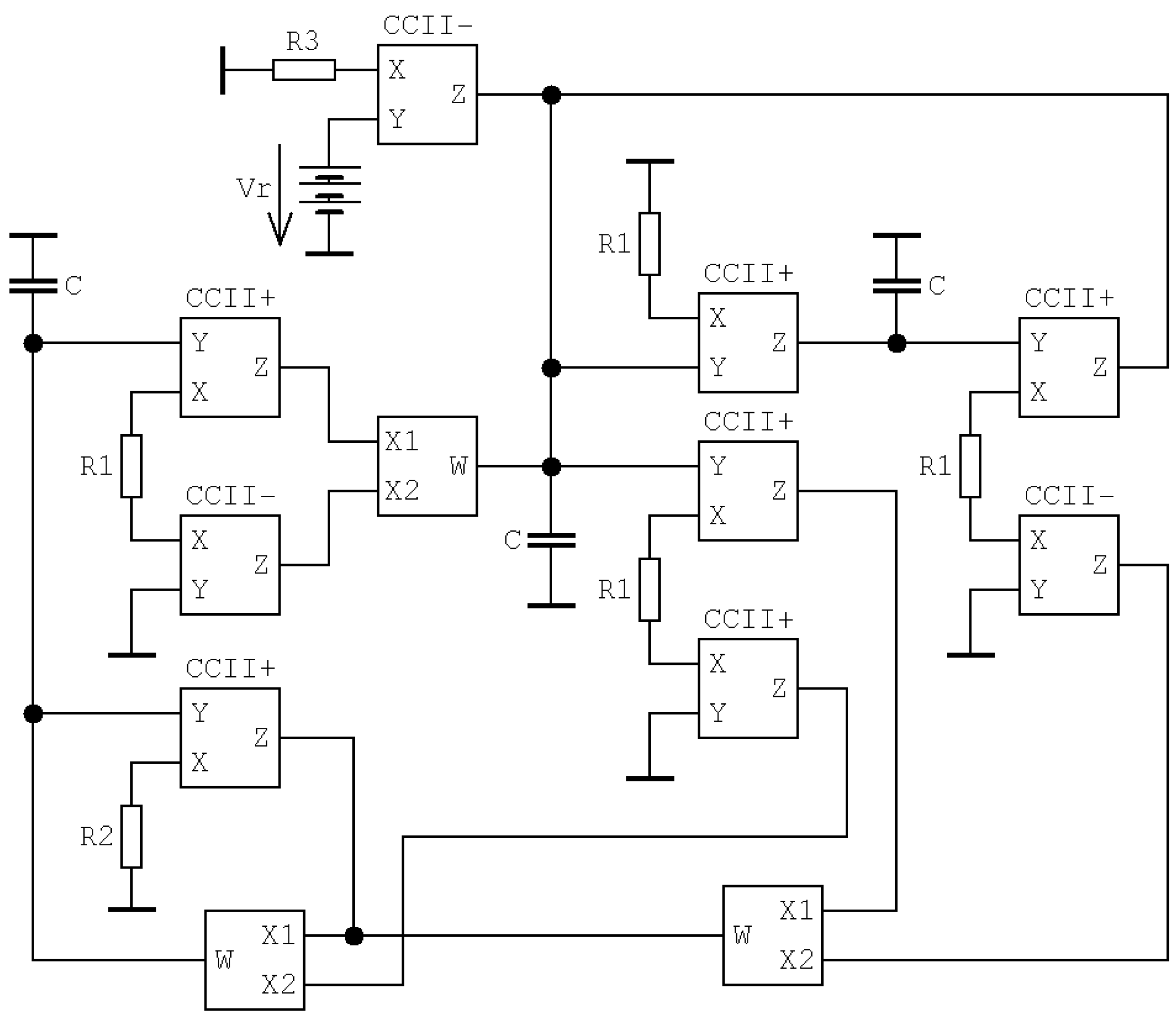
Circuitry implementation of the dynamical system (1) working in voltage- and current-mode is given in
Figure 6 and
Figure 7 respectively. Let us discuss the first realization in more detail. Note that the inevitable price for the complex mathematical model is many active elements; one TL084 with four standard voltage-feedback operational amplifiers in a single package and three four-quadrant analog multipliers AD633 with transfer function
VW =
K(
VX1 −
VX2)(
VY1 −
VY2) +
VZ are required. Both types of the active elements are fed by a symmetrical ±15 V voltage supply. This creates sufficient dynamical range for bounded types of the state space attractors. Chaotic signals can be directly measured at the outputs of inverting integrators where state variables
x,
y and −
z can be found. Describing the set of differential equations of the circuit shown in
Figure 6 can be expressed as
where
K = 0.1 is an internally trimmed constant associated with each analog multiplier and
Vr = 1 V is a fixed voltage, which can be directly derived from the positive voltage supply by a resistor-based voltage divider followed by a voltage buffer. To obtain chaotic waveforms, we can choose the following numerical values of passive circuit components:
C = 100 nF,
R1 = 10 kΩ,
R2 = 1 kΩ,
R3 = 830 Ω (potentiometer, set of parameter
a) and
R4 = 2500 Ω (potentiometer, set of parameter
b).
In the case of the current-mode chaotic oscillator, the unity gain factor of the integrated circuit EL2082 (which can be naturally adjusted by an external dc voltage between zero and two, see datasheet for details) is supposed, while the integrated circuit AD844 has unity current gain automatically. On the other hand, the gain factor of the
k-th current multiplier is arbitrary and denoted as
Bk. Transfer function of the
k-th multiplier can be expressed simply as
IW =
Bk·
IX·
IY. The set of differential equations, which fully covers network realization shown in
Figure 7 is in the form:
where
Vr = 1 V is the dc voltage dedicated to change the offset of the hyperbolic function. Note that summing operation is realized by a single node. Supply voltage does not need to be lowered, since AD844, EL2082, as well as EL4083 can operate with symmetrical ±15 V. It is evident that twelve active elements are needed for the design of this chaotic oscillator using discrete components. However, such a principle will probably be chosen in the case of full on-chip implementation, using available CMOS technology. Practical realization of the prescribed chaotic attractor can be problematic if the fabrication of technology does not support a sufficiently wide range of the supply voltages.
3.1. Note on Parasitic Properties of Active Elements and Existence of Chaotic Attractor
It is well known that the typical parasitic properties of the active elements (at least those utilized here for the design of oscillators) are input and output impedances which, especially when at high frequency bands, can no longer be supposed to be infinite or zero. Analysis of the effects of parasitic features sometimes also includes the roll-off nature of transfer constants. In the case of analog filters [
31] or oscillators [
32], all mentioned non-ideal properties of active elements can be directly included into semi-symbolic formulas, which describe the fundamental function of a designed building block. Unfortunately, this concept cannot be used for a chaotic oscillator because the immediate impact of particular parasitic ingredients on the global dynamical flow cannot be predicted; there is no formula (function of circuit parameters) for the existence of a strange attractor.
The answer to this question can be found in the calculation of LE, rendering it a truly numerical problem. Note, such analysis is possible only if we can include all necessary parasitic properties into the original mathematical model, that is, describing a set of ordinary differential equations. Results can be reformulated as follows: what are the maximum values of parasitic properties to get a chaotic attractor with a prescribed metric dimension? Achieved concluding remarks are topology-specific; that is, different circuit implementations of the same dynamical system can (and will) exhibit various sensitivities to non-ideal features of the active devices. Thus, after performing the mentioned calculations, we can mark some of the designs that are optimal in this sense and more suitable for practical applications. The design with the minimum number of active elements will probably be the optimal one.
3.2. Orcad Pspice Simulation Results and Oscilloscope Screenshots
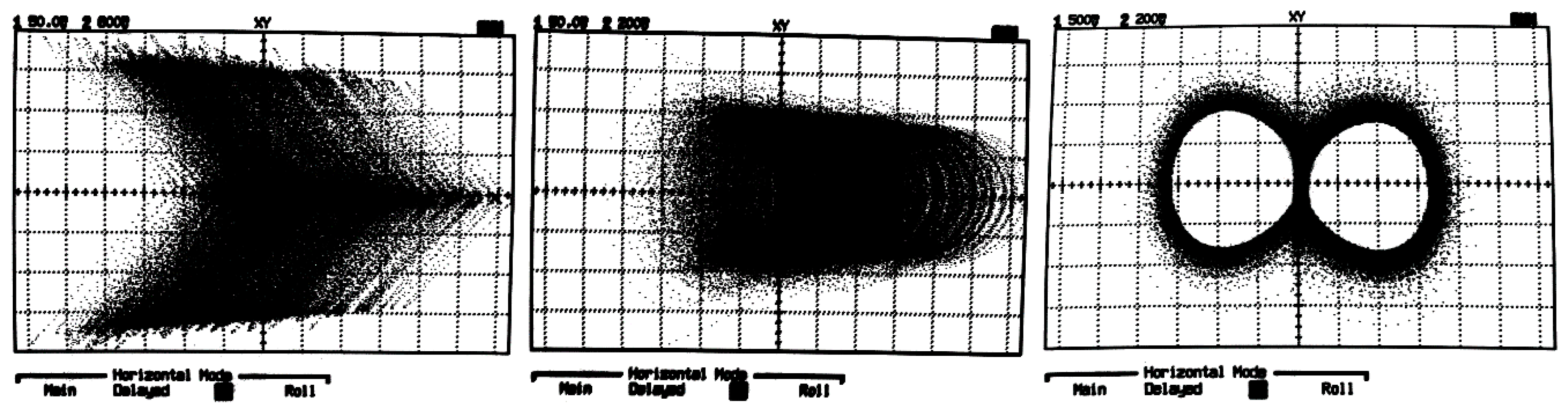
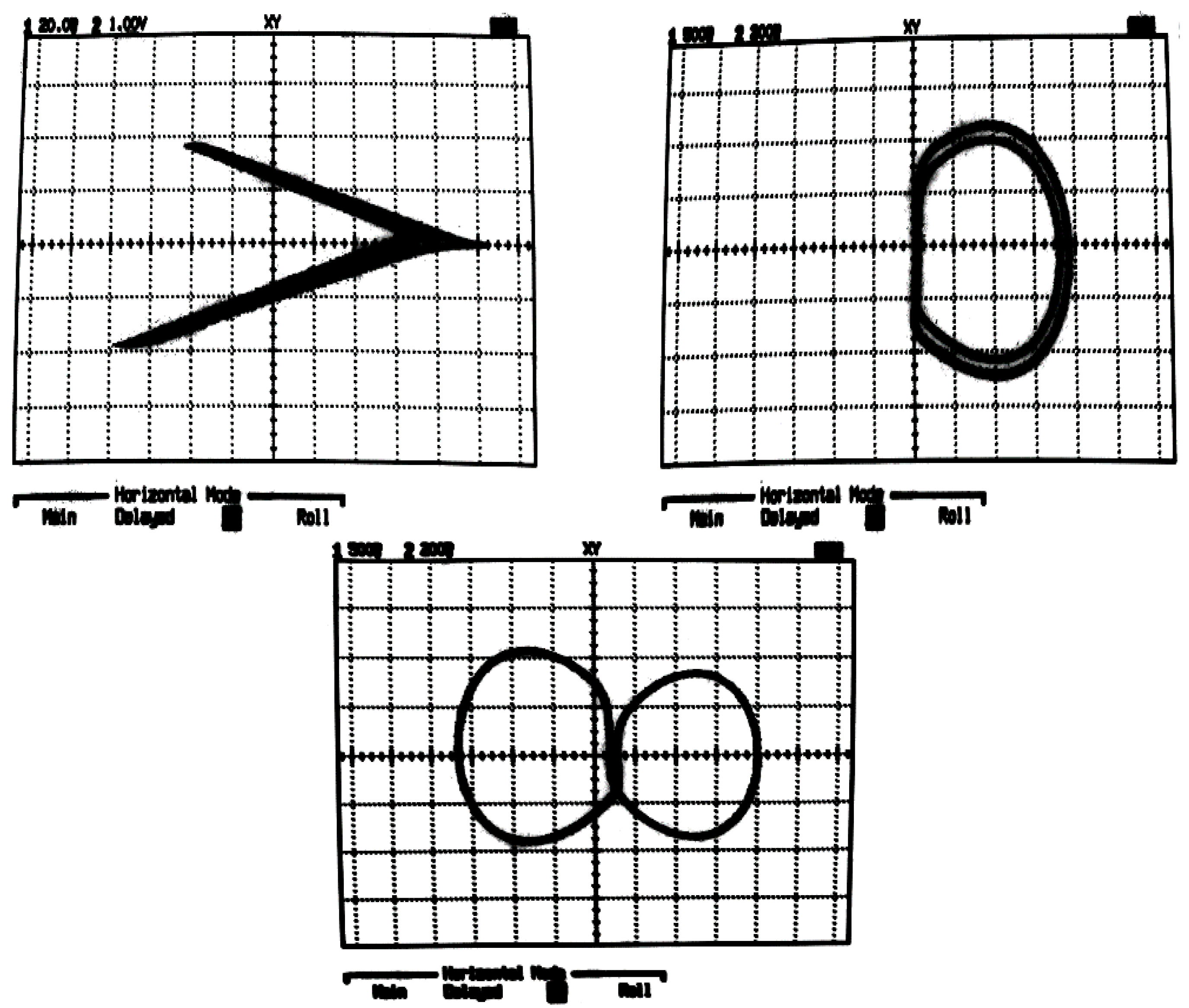
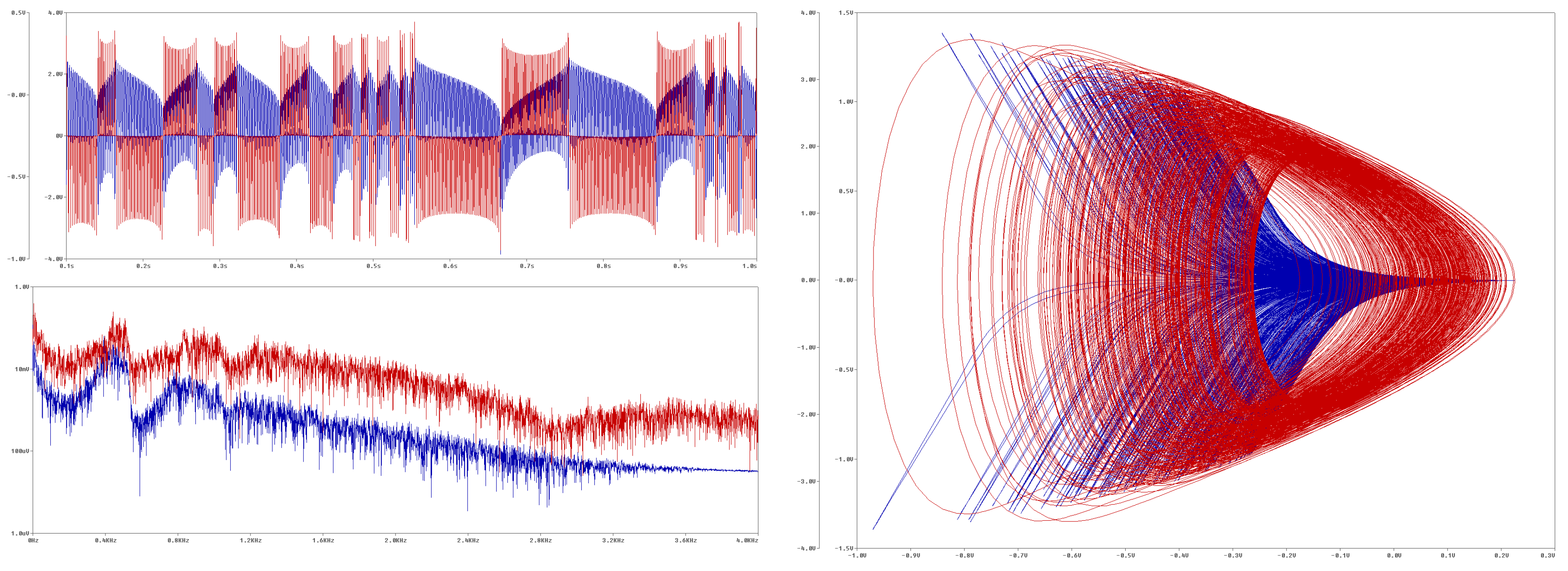
The common standard is to prove the existence of a structurally stable chaotic attractor by experimental measurement, that is, by showing oscilloscope screenshots. Monge’s plane projections of a typical chaotic attractor captured by a digital oscilloscope HP54603B are illustrated in
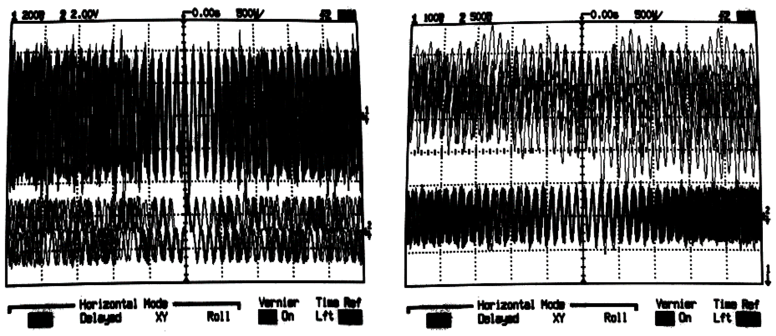
Figure 8 and the chaotic waveforms in the time domain are demonstrated in
Figure 9. Surprisingly, real measurement uncovers a kind of behavior that has not been revealed by the numerical approach; namely the limit cycle visible in
Figure 10. The inverse approach, that is, the transformation of the circuit values into mathematical model parameters, fails to provide a similar numerically integrated limit cycle. Chaotic oscillators are very sensitive to the circuit parameters, so much so that a detailed bifurcation scenario such as period doubling (or another form of routing-to-chaos sequence) has not been captured and seems to be handmade and unmeasurable. The current-mode configuration of the chaotic oscillator has been briefly verified by an Orcad Pspice circuit simulator and corresponding results are shown in
Figure 11.
4. Discussion
The proposed mathematical model represents a new contribution to the class of dynamical systems with hyperbolic equilibrium listed in [
26], that is, the mathematical models with an infinite number of equilibrium points that are arranged into a curved object. The hidden chaotic attractor, namely the double-funnel-like geometrical structure (for clarification, please refer to the well-known Rossler attractor for a single-funnel) is experimentally revealed by the imposing-the-state technique: very short impulse voltages are directly connected to nodes which represent state variables simultaneously. However, long-term stability of the strange attractor is rather problematic due to power consumption and component heating (values of circuit parameters change and the chaotic attractor eventually disappears). A very good overall relation between numerical analysis and experimental measurement is demonstrated.
There are many numerical applications of algorithms rising from recent advances in nonlinear time series analysis. The spectrum of LE was used to qualitatively describe dynamical flow and distinguish between chaotic and non-chaotic dynamics, which can be utilized to calculate the so-called Kaplan–Yorke dimension of the state space attractor [
33]. This single real number can be adopted in routine for optimal approximation of the polynomial chaotic dynamics. Some simple examples can be found in [
34].
A more detailed analysis of the introduced mathematical model, with respect to the chaos evolution principle, leaves room for future research. Advancements towards fourth-order hyperchaotic systems with equilibria in the form of a three-dimensional geometrical structure (cuboid, sphere, etc.) can be expected in the upcoming years.


